A general construction for parallelizing Metropolis−Hastings algorithms

Significance

Many computational problems in modern-day statistics are heavily dependent on Markov chain Monte Carlo (MCMC) methods. These algorithms allow us to evaluate arbitrary probability distributions; however, they are inherently sequential in nature due to the Markov property, which severely limits their computational speed. We propose a general approach that allows scalable parallelization of existing MCMC methods. We do so by defining a finite-state Markov chain on multiple proposals in a way that ensures asymptotic convergence to the correct stationary distribution. In example simulations, we demonstrate up to two orders of magnitude improvement in overall computational performance.

Abstract

Markov chain Monte Carlo methods (MCMC) are essential tools for solving many modern-day statistical and computational problems; however, a major limitation is the inherently sequential nature of these algorithms. In this paper, we propose a natural generalization of the Metropolis−Hastings algorithm that allows for parallelizing a single chain using existing MCMC methods. We do so by proposing multiple points in parallel, then constructing and sampling from a finite-state Markov chain on the proposed points such that the overall procedure has the correct target density as its stationary distribution. Our approach is generally applicable and straightforward to implement. We demonstrate how this construction may be used to greatly increase the computational speed and statistical efficiency of a variety of existing MCMC methods, including Metropolis-Adjusted Langevin Algorithms and Adaptive MCMC. Furthermore, we show how it allows for a principled way of using every integration step within Hamiltonian Monte Carlo methods; our approach increases robustness to the choice of algorithmic parameters and results in increased accuracy of Monte Carlo estimates with little extra computational cost.

Since its introduction in the 1970s, the Metropolis−Hastings algorithm has revolutionized computational statistics (1). The ability to draw samples from an arbitrary probability distribution, $\pi \left(X\right)$, known only up to a constant, by constructing a Markov chain that converges to the correct stationary distribution has enabled the practical application of Bayesian inference for modeling a huge variety of scientific phenomena, and has resulted in Metropolis−Hastings being noted as one of the top 10 most important algorithms from the 20th century (2). Despite regular increases in available computing power, Markov chain Monte Carlo (MCMC) algorithms can still be computationally very expensive; many thousands of iterations may be necessary to obtain low-variance estimates of the required quantities with an oftentimes complex statistical model being evaluated for each set of proposed parameters. Furthermore, many Metropolis−Hastings algorithms are severely limited by their inherently sequential nature.

Many approaches have been proposed for improving the statistical efficiency of MCMC, and although such algorithms are guaranteed to converge asymptotically to the stationary distribution, their performance over a finite number of iterations can vary hugely. Much research effort has therefore focused on developing transition kernels that enable moves to be proposed far from the current point and subsequently accepted with high probability, taking into account, for example, the correlation structure of the parameter space (3, 4), or by using Hamiltonian dynamics (5) or diffusion processes (6). A recent investigation into proposal kernels suggests that more exotic distributions, such as the Bactrian kernel, might also be used to increase the statistical efficiency of MCMC algorithms (7). The efficient exploration of high-dimensional and multimodal distributions is hugely challenging and provides the motivation for many further methods (8).

Computational efficiency of MCMC algorithms is another important issue. Approaches have been suggested for making use of the increasingly low-cost parallelism that is available in modern-day computing, with the most straightforward based on running multiple Markov chains simultaneously (9). These may explore the same distribution, or some product of related distributions, as in parallel tempering (10). Furthermore, the locations of other chains may additionally be used to guide the proposal mechanism (11). More recent work combines the use of multiple chains with adaptive MCMC in an attempt to use these multiple sources of information to learn an appropriate proposal distribution (12, 13). Sometimes, specific MCMC algorithms are directly amenable to parallelization, such as independent Metropolis−Hastings (14) or slice sampling (15), as indeed are some statistical models via careful reparameterization (16) or implementation on specialist hardware, such as graphics processing units (GPUs) (17, 18); however, these approaches are often problem specific and not generally applicable. For problems involving large amounts of data, parallelization may in some cases also be possible by partitioning the data and analyzing each subset using standard MCMC methods simultaneously on multiple machines (19). The individual Markov chains in these methods, however, are all based on the standard sequential Metropolis−Hastings algorithm.

The idea of parallelizing Metropolis−Hastings using multiple proposals has been investigated previously; however, the main shortcoming of such attempts has been their lack of computational efficiency. Algorithms such as Multiple Try Metropolis (20), Ensemble MCMC (21), and “prefetching” approaches (22, 23) all allow the computation of multiple proposals or future proposed paths in parallel, although only one proposal or path is subsequently accepted by the Markov chain, resulting in wasted computation of the remaining points. Another class of approaches involves incorporating rejected states into the Monte Carlo estimator with an appropriate weighting, such that the resulting estimate is still unbiased. An overview of such approaches is given by Frenkel (24). In particular, the work presented by Tjelmeland (25) makes use of multiple rejected states at each iteration and is related to the ideas presented here, although recent investigations suggest that including all rejected proposals may in fact sometimes result in a Monte Carlo estimate with asymptotically larger variance than using only accepted states (26).

In this paper, we present a generalization of Metropolis−Hastings that may be used to parallelize a wide variety of existing MCMC algorithms, including most of those mentioned previously, from simple random-walk Metropolis to more recent Langevin-based algorithms, defined either on Euclidean or Riemannian spaces, and Adaptive MCMC. The approach we propose is highly scalable and may offer a couple of magnitudes improvement in time-normalized efficiency over existing algorithms. The approach offers additional practical benefit for Hamiltonian Monte Carlo (HMC) methods, by improving robustness to the choice of tuning parameters and providing a principled way of making use of the intermediate integration steps that are calculated at every iteration.

Metropolis−Hastings for a Single Proposed Point

The original Metropolis algorithm is straightforward to understand since it is implemented with a symmetric proposal distribution (27). If the probability at the proposed point is greater than at the current point, the move is always accepted. Otherwise, it is only accepted with probability proportional to the ratio of the new point and the old point; intuitively, it is visited less often to ensure that the long-term frequency of visits is proportional to its underlying probability. The extension by Hastings (28) ensures convergence to the correct stationary distribution when using nonsymmetric proposals; the new acceptance ratio effectively removes the bias introduced by the fact that now some reverse moves will have a different probability of being proposed than the forward move.

Let $K\left(x_i,x_j\right)$ be a Markov chain on a state space X, defined by a possibly nonsymmetric proposal distribution conditioned on the current point $x_i$. A useful interpretation of the Metropolis−Hastings algorithm (29) is that we wish to turn the Markov chain K into another Markov chain that has the stationary distribution, $\pi \left(X\right)$. According to the Metropolis−Hastings algorithm, we propose a move from $x_i$ to $x_j$ with probability $K\left(x_i,x_j\right)$ and then accept this move with some probability $A\left(x_i,x_j\right)\in \left[\mathrm{0,1}\right]$. We observe that $A\left(\cdot ,\cdot \right)$ here may also be considered as a Markov chain. The product of these Markov chains, $K\left(x_i,x_j\right)A\left(x_i,x_j\right)$, $\left(x_i\ne x_j\right)$, converges to the desired stationary distribution if it is reversible,

$$\pi \left(x_i\right)K\left(x_i,x_j\right)A\left(x_i,x_j\right)=\pi \left(x_j\right)K\left(x_j,x_i\right)A\left(x_j,x_i\right),$$ [1]

which is an easy to satisfy, sufficient condition for the necessary balance condition to hold,

$$\pi \left(x_i\right)={\displaystyle \int \pi \left(x_j\right)K\left(x_j,x_i\right)A\left(x_j,x_i\right)d{x}_j}.$$ [2]

For any two states $x_i$ and $x_j$, we have from Eq. 1,

$$A\left(x_j,x_i\right)=\frac{1}{R\left(x_i,x_j\right)}A\left(x_i,x_j\right)\le 1,$$ [3]

where $R\left(x_i,x_j\right)=\frac{\pi \left(x_j\right)K\left(x_j,x_i\right)}{\pi \left(x_i\right)K\left(x_i,x_j\right)}$. From this, a general form for acceptance probabilities for reversible Metropolis−Hastings algorithms (29) follows as, $0\le A\left(x_i,x_j\right)\le \min \left(1,R\left(x_i,x_j\right)\right)$, since $A\left(x_i,x_j\right)\le R\left(x_i,x_j\right)$ from the inequality in Eq. 3. Taking $A\left(x_i,x_j\right)$ to be its maximum, we recover the optimal Metropolis−Hastings acceptance probability (30).

It is straightforward to see that by proposing a point $x_j$ from the transition kernel $K\left(x_i,\mathrm{\cdot }\right)$, and accepting with probability $A\left(x_i,x_j\right)$, detailed balance is satisfied and the chain retains the correct stationary distribution. It is important at this stage to realize that when we accept or reject the proposed step, we are in fact simulating from the finite state Markov chain $A\left(\cdot ,\cdot \right)$. The traditional Metropolis−Hastings approach results in a single step being taken at each iteration based on the two-state Markov chain shown in Fig. 1, and we note that since only one transition within this finite-state Markov chain is made, the remaining transition probabilities $A\left(x_j,\cdot \right)$ are not immediately used.

Fig. 1.

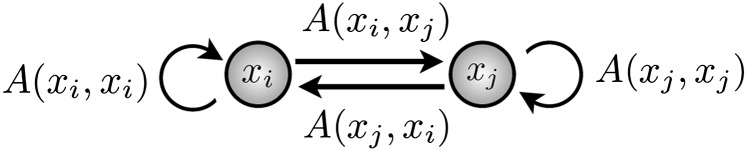
A two-state Markov chain corresponding to a single step taken using the standard Metropolis−Hastings algorithm. Starting at $x_i$, a single step is made and the chain either moves to $x_j$ or remains at $x_i$. We note that the other transition probabilities $A\left(x_j,x_i\right)$ and $A\left(x_j,x_j\right)$ are not directly used.

Metropolis−Hastings for Multiple Proposed Points

We now consider the case where we define our Markov chain, $A\left(\cdot ,\cdot \right)$, over multiple proposed states and show that this may also be constructed to obtain a sampling algorithm that has the correct stationary distribution. A useful representation for deriving and proving the validity of this approach is as a Metropolis−Hastings algorithm defined over a product space. We first note that a joint distribution $p\left(x_{1:N+1}\right)$ may be factorized in $N+1$ different ways using the form, $p\left(x_{1:N+1}\right)=p\left(x_i\right)p\left(x_{\mathrm{\setminus }i}|x_i\right)\equiv \pi \left(x_i\right)K\left(x_i,x_{\mathrm{\setminus }i}\right)$, where we use the notation $K\left(x_i,x_{\mathrm{\setminus }i}\right)=p\left(x_{\left[1:i-1,i+1:N+1\right]}|x_i\right)$. We observe that the ith factorization is defined such that $x_i$ is distributed according the target density of interest, and the other points, $x_{\mathrm{\setminus }i}$, are distributed according to a proposal kernel conditioned on the ith point. Following Tjelmeland (25), we may introduce a discrete uniform auxiliary random variable I defined over the integers $\left[1:N+1\right]$, indicating which factorization of this joint probability distribution should be used, i.e., $p\left(x_{1:N+1},I=i\right)=\frac{1}{N+1}p\left(x_i\right)p\left(x_{\mathrm{\setminus }i}|x_i\right)$.

The Generalized Metropolis−Hastings algorithm, which we describe shortly, is equivalent to a single Markov chain exploring the product space $p\left(x_{1:N+1},I\right)$, using a combination of two different transition kernels, each of which preserves the underlying joint stationary distribution. First, we update the variables $x_{\mathrm{\setminus }i}$ conditioned on $x_i$ and $I=i$, which clearly preserves the correct stationary distribution, since we can sample directly from the proposal kernel $K\left(x_i,\mathrm{\cdot }\right)$. We note that we are free to choose the form of this proposal kernel, and, later in the paper, we consider the use of kernels based on Langevin diffusions and Hamiltonian dynamics. Secondly, we sample the auxiliary variable I conditioned on the current states $x_{1:N+1}$, using the transition matrix $A\left(\cdot ,\cdot \right)$, where $A\left(i,j\right)$ defines the probability of transitioning from $I=i$ to $I=j$. We see that by construction, when $I=i$, the random variable $x_i$ has the correct target density $\pi \left(x_i\right)$, and these are the samples we collect at each iteration. Furthermore, we may calculate the stationary distribution of the transition matrix, which we denote as $A^{\infty }$, and use this to sample I directly. There are two sources of increased efficiency that arise from the Generalized Metropolis−Hastings algorithm; the first is that the likelihoods of the multiple proposed points may be computed in parallel, and the second is that the acceptance rate is increased when using multiple proposals.

We now give an algorithmic overview, before deriving appropriate transition probabilities and proving that the balance condition is satisfied. The Generalized Metropolis−Hastings algorithm proceeds as follows.

• 1:Initialize starting point ${\tilde{x}}_1$, auxiliary variable $I=1$ and counter $n=0$.
• 2:for each MCMC iteration do
• 3:Update ${\tilde{x}}_{\mathrm{\setminus }I}$ conditioned on I, i.e., draw N new points from the proposal kernel $p\left({\tilde{x}}_{\mathrm{\setminus }I}|{\tilde{x}}_I\right)=K\left({\tilde{x}}_I,\mathrm{\cdot }\right)$.
• 4:Calculate the stationary distribution of I conditioned on ${\tilde{x}}_{1:N+1}$, i.e., $\forall j\in \left[1,\hspace{0.17em}\dots ,\hspace{0.17em}N+1\right]$, $p\left(I=j|{\tilde{x}}_{1:N+1}\right)=A^{\infty }\left(\cdot ,j\right)\propto \pi \left({\tilde{x}}_j\right)K\left({\tilde{x}}_j,{\tilde{x}}_{\mathrm{\setminus }j}\right)$, which follows from Eq. 5 and may be calculated in parallel.
• 5:for m = 1:N do
• 6:Sample directly from the stationary distribution of the auxiliary variable, I, to obtain the sample, $x_{n+m}={\tilde{x}}_I$.
• 7:end for
• 8:Update counter, $n=n+N$.
• 9:end for

We note that for $N=1$, the algorithm simplifies to the original Metropolis−Hastings algorithm, with a single proposed point and a single sample drawn at each iteration. In the algorithm above, we chose to sample N times, although this need not necessarily equal the number of proposals. We shall now derive all transition probabilities for the matrix $A\left(\cdot ,\cdot \right)$, such that the balance condition is satisfied over the product space. We begin by noting that the detailed balance condition for updating the variable I in this product space is

$$\frac{1}{N+1}\pi \left(x_i\right)K\left(x_i,x_{\mathrm{\setminus }i}\right)A\left(i,j\right)=\frac{1}{N+1}\pi \left(x_j\right)K\left(x_j,x_{\mathrm{\setminus }j}\right)A\left(j,i\right),$$ [4]

for all i and j, and the balance condition follows as

$$\frac{1}{N+1}\pi \left(x_i\right)K\left(x_i,x_{\mathrm{\setminus }i}\right)={\displaystyle \sum _{j=1}^{N+1}\frac{1}{N+1}\pi \left(x_j\right)K\left(x_j,x_{\mathrm{\setminus }j}\right)A\left(j,i\right)},$$ [5]

for all i. We can now derive a similar expression for the transition probabilities as we did in the single proposal case.

Proposition 1. We may construct a finite-state Markov chain $A\left(\cdot ,\cdot \right)$ defining the transition probabilities for I given the current set of states $x_{1:N+1}$ using

$$A\left(i,j\right)=\{\begin{array}{ll}\frac{1}{N}\min \left(1,R\left(i,j\right)\right),\hfill & if\hspace{0.17em}j\ne i,\hfill \\ 1-{\displaystyle {\sum }_{j\ne i}A\left(i,j\right)},\hfill & otherwise,\hfill \end{array}$$ [6]

where

$$R\left(i,j\right)=\frac{\pi \left(x_j\right)K\left(x_j,x_{\mathrm{\setminus }j}\right)}{\pi \left(x_i\right)K\left(x_i,x_{\mathrm{\setminus }i}\right)}.$$ [7]

Each transition of this Markov chain, $A\left(i,\mathrm{\cdot }\right)$, satisfies the detailed balance and balance conditions (Eqs. 4 and 5). The joint distribution $p\left(X_{1:N+1},I\right)$ is therefore invariant when the variable I is sampled using such updates.

From the reversibility condition for each pair of values $\left[I=i,I=j\right]$ we have, $0\le A\left(i,j\right)\le \min \left(1,R\left(i,j\right)\right),\left(j\ne i\right)$, where R is now given by Eq. 7. In order for $A\left(\cdot ,\cdot \right)$ to be a Markov chain, we also require that ${\displaystyle {\sum }_{j=1}^{N+1}A\left(i,j\right)}=1$ and $A\left(i,i\right)=1-{\displaystyle {\sum }_{j\ne i}A\left(i,j\right)}\ge 0$. When $N>1$, we may try to satisfy these requirements for $A\left(\cdot ,\cdot \right)$ by considering weights $c_j\in \left[\mathrm{0,1}\right]$ such that $0\le A\left(i,j\right)\le c_j\min \left(1,R\left(i,j\right)\right),\left(j\ne i\right)$. If we choose $A\left(i,j\right)$ to maximize this inequality, then the reversibility condition in Eq. 4 implies that $c_j=c_i$, i.e., we may choose a constant c for all proposed points. We therefore have ${\displaystyle {\sum }_{j\ne i}c\min \left(1,R\left(i,j\right)\right)}\le 1$. Taking the maximum of this quantity implies that ${\displaystyle {\sum }_{j\ne i}c}\le 1$ and so letting $c=1/N$ satisfies this inequality. It is therefore now clear that $A\left(\cdot ,\cdot \right)$, defined in Eq. 6, is a Markov chain that satisfies the detailed balance condition in Eq. 4, and hence also the balance condition in Eq. 5, from which the stationary distribution of $A\left(\cdot ,\cdot \right)$ directly follows.

We note that the acceptance ratio depends on both the current point and all proposed points, and consequently the probability of transitioning from $I=i$ to $I=j$ may become very small. For this reason, we may use a similar approach as presented in ref. 25, whereby we introduce an auxiliary variable z and make proposals of the form, $\tilde{K}\left(x_i,x_{\mathrm{\setminus }i}\right)=K\left(x_i,z\right)K\left(z,x_{\mathrm{\setminus }i}\right)$. The acceptance ratio then simplifies to

$$R\left(i,j\right)=\frac{\pi \left(x_j\right)\tilde{K}\left(x_j,x_{\mathrm{\setminus }j}\right)}{\pi \left(x_i\right)\tilde{K}\left(x_i,x_{\mathrm{\setminus }i}\right)}=\frac{\pi \left(x_j\right)K\left(x_j,z\right)K\left(z,x_i\right)}{\pi \left(x_i\right)K\left(x_i,z\right)K\left(z,x_j\right)},$$ [8]

and, for symmetric proposals, the acceptance rate simplifies further to $R\left(i,j\right)=\pi \left(x_j\right)/\pi \left(x_i\right)$.

Materials and Methods

We now detail the MCMC algorithms, statistical models, and measures of efficiency that we use for investigating the numerical performance of this generalized construction of Metropolis−Hastings. For the simulations, we adopt the Bayesian approach, such that our target density is the posterior distribution, $\pi \left(x\right)=p\left(x|y\right)\propto p\left(y|x\right)p\left(x\right)$. We can therefore draw samples from the posterior distribution using Metropolis−Hastings without explicitly having to calculate the normalizing constant, given by the marginal likelihood, $p\left(y\right)$.

Metropolis-Adjusted Langevin Algorithms.

Continuous-time stochastic differential equations that converge to the correct stationary distribution may be used to make efficient moves within MCMC algorithms; however, a Metropolis−Hastings correction step is still required, since the discretized solution no longer converges to the correct distribution. Such an approach works well, as it takes into account the local geometry of the target density. Original versions of Metropolis-Adjusted Langevin Algorithms (MALA) were based on a diffusion defined in Euclidean space (6), although recently it has been shown that they may also be defined on the Riemannian manifold induced by the statistical model (4). In the Riemannian case, the resulting proposal mechanism has a position-specific covariance matrix defined by the expected Fisher Information, which satisfies the properties of a metric tensor (31); the resulting Markov chain therefore proposes transitions by taking into account at each step the average local sensitivity of the statistical model with respect to small changes in its parameters. Computationally efficient proposals may be made using the following simplified manifold MALA (SmMALA) transition kernel (4), which we use for the subsequent numerical simulations in this paper, $K\left(x_i,\mathrm{\cdot }\right)=\mathcal{N}\left(x_i+\left({\mathit{ϵ}}^2/2\right)G{\left(x_i\right)}^{-1}{\nabla }_x\log p\left(x_i|y\right),{\mathit{ϵ}}^{2}G{\left(x_i\right)}^{-1}\right)$, where $G\left(x_i\right)$ is the position-specific covariance matrix given by the expected Fisher Information (4).

Adaptive MCMC.

An alternative approach is to adaptively learn an appropriate proposal covariance structure based on previously accepted MCMC moves. Convergence to the stationary distribution must be proven separately for this class of algorithms, since the chain is no longer Markovian (3). For the purpose of our simulation study, we use the Langevin-based Adaptive MCMC algorithm detailed in ref. 32. The transition kernel is given as $K\left(x_i,\cdot \right)=\mathcal{N}\left(x_i+\left({\mathit{ϵ}}^2/2\right)\mathrm{\Lambda }D\left(x_i\right),{\mathit{ϵ}}^2\mathrm{\Lambda }\right)$, where $D\left(x_i\right)=\left[\delta /\max \left(\delta ,\left|\nabla \log p\left(x_i|y\right)\right|\right)\right]\nabla \log p\left(x_i|y\right)$ is the bounded drift function, with δ a fixed constant and the covariance matrix $\Lambda$ computed at each iteration based on the previously accepted moves with diminishing adaptation (32), such that the chain asymptotically converges to the correct stationary distribution. This Adaptive MCMC algorithm may be straightforwardly implemented with the proposed Generalized Metropolis−Hastings approach by simply updating the covariance matrix after every iteration, i.e., after N points have been proposed and sampled.

HMC.

We may augment the posterior distribution with an auxiliary Gaussian random variable and interpret the negative joint log density as a Hamiltonian system (5), $H\left(x,p\right)=-\log p\left(x|y\right)+\left(1/2\right)\log \left({\left(2\pi \right)}^D\left|M\right|\right)+\left(1/2\right)p^T{M}^{-1}p$, where M is the mass matrix defining the covariance structure of the “momentum” auxiliary variable p. Hamiltonian dynamics may then be used to inform a transition kernel that takes into account the local geometry of the posterior, proposing moves far from the current point that may be accepted with high probability. However, for most statistical models, the Hamiltonian dynamics are not analytically tractable and must be numerically approximated using a symplectic, time-reversible integrator (33), with the discretization error subsequently corrected using a Metropolis−Hastings step. Here we use the Euclidean version of HMC using the Leapfrog integrator, although we note that this may also be defined on the induced Riemannian manifold of the statistical model (4). We wish to sample from the target density $\pi \left(x,p\right)=\exp \left(-H\left(x,p\right)\right)$. We propose a transition by sampling an initial momentum variable from a normal distribution, $N\left(0,M\right)$, then deterministically calculating the mapping $\left[x,p\right]\to \left[x^{*},p^{*}\right]$ using a number of numerical integration steps, each of which is defined by

$$p\left(\tau +\mathit{ϵ}/2\right)=p\left(\tau \right)+\mathit{ϵ}\nabla \log p\left(x\left(\tau \right)|y\right)/2$$

$$x\left(\tau +\mathit{ϵ}\right)=x\left(\tau \right)+\mathit{ϵ}{M}^{-1}p\left(\tau +\mathit{ϵ}/2\right)$$

$$p\left(\tau +\mathit{ϵ}\right)=p\left(\tau +\mathit{ϵ}/2\right)+\mathit{ϵ}\nabla \log p\left(x\left(\tau +\mathit{ϵ}\right)|y\right)/2.$$

In standard Metropolis−Hastings, only the end point of the integration path is used as the proposal. With Generalized Metropolis−Hastings, we can make use of all intermediate integration steps by considering them as multiple Hamiltonian proposals. It is straightforward to obtain a suitable transition kernel for HMC in this setting by randomly sampling the number of integration steps from a discrete uniform distribution, $s\sim U\left(1,S\right)$, and calculating the Hamiltonian path s steps forward in time and $S-s$ steps backward from the current point. This results in a symmetric proposal from each point to the set of all other points in the Hamiltonian path, such that we may use the simplified acceptance ratio, $R\left(i,j\right)=\pi \left(x_j,p_j\right)/\pi \left(x_i,p_i\right)$, to define the transition probabilities for the auxiliary variable I.

Calculating the Sampling Efficiency.

The samples generated using MCMC exhibit some level of autocorrelation, due to the Markov property. One way of evaluating the statistical efficiency of such methods is by calculating the effective sample size (ESS), which is the number of effectively independent samples from the total number of posterior samples collected. For each covariate, we may use the following standard measure, $\text{ESS}=N{\left[1+2{\displaystyle {\sum }_k\gamma \left(k\right)}\right]}^{-1}$, where N is the number of posterior samples and ${\displaystyle {\sum }_k\gamma \left(k\right)}$ is the sum of the K monotone sample autocorrelations, estimated by the initial monotone sequence estimator (34). An alternative approach is to consider the mean squared jumping distance, $\text{MSJD}=\left(1/N\right){\displaystyle {\sum }_{n=1}^{N-1}{\Vert x_{n+1}-x_n\Vert }^2}$, which is related to measuring the lag 1 autocorrelation and may furthermore be used to optimize the parameters of the proposal kernel (35). We make use of both of these measures to investigate the performance of Generalized Metropolis−Hastings.

Ordinary Differential Equation Models.

Statistical models based on systems of ordinary differential equations (ODEs) have a wide range of scientific uses, from describing cell regulatory networks, to large-scale chemical processes and inference in such mechanistic models presents many challenges, both due to the computational effort involved in evaluating the solution for each set of proposed parameters, as well as the challenge of sampling from potentially strongly correlated posterior distributions, resulting from any nonlinearities present in the model equations. We consider ODEs of the form $\dot{u}=f\left(u,\theta \right)$, which we solve numerically for the implicitly defined solution states u. Given uncertain measurements of each solution state $y_i=u_i+{\gamma }_i$, with γ defined according to the chosen error model, we wish to infer the posterior distribution over the model parameters θ. We use the Fitzhugh−Nagumo model as an illustrative example of such a system (4), which consists of two states, $\dot{V}=c\left(V-V^3/3+R\right)$ and $\dot{R}=-\left(V-a+bR\right)/c$. Following ref. 4, we use 200 data points generated from the Fitzhugh−Nagumo ODE model between $t=0$ and $t=20$ inclusive, with model parameters $a=0.2$, $b=0.2$, and $c=3$ and initial conditions $V_0=-1$ and $R_0=1$. Gaussian-distributed error with SD equal to 0.5 was then added to the data, which was subsequently used for inference of the model parameters.

Logistic Regression Models.

We also consider a Bayesian logistic regression example defined by an $N\times D$ design matrix, X, where N is the number of samples, each described using D covariates, such that $p\left(y=1|X,\theta \right)=\sigma \left(X\theta \right)$ and $p\left(y=0|X,\theta \right)=1-\sigma \left(X\theta \right)$, where σ denotes the logistic function. We perform inference over the regression coefficients $\theta \in {\mathrm{ℝ}}^D$ by defining Gaussian priors $p\left(\theta \right)=\mathcal{N}\left(0,\alpha I\right)$, with $\alpha =100$. For implementing SmMALA, the metric tensor for this model follows straightforwardly as $G\left(\theta \right)=X^T\mathrm{\Lambda }X+\alpha I$, where $\mathrm{\Lambda }$ is a diagonal matrix with elements ${\mathrm{\Lambda }}_{\left(n,n\right)}=\sigma \left({\theta }^T{X}_{\left(n,\mathrm{\cdot }\right)}^T\right)\left(1-\sigma \left({\theta }^T{X}_{\left(n,\mathrm{\cdot }\right)}^T\right)\right)$; see ref. 4 for further details.

Results

Statistical Efficiency with Increasing Number of Proposals.

We investigate the statistical efficiency of Generalized Metropolis−Hastings using increasing numbers of proposals. Once N proposals have been selected, the likelihood and transition probabilities may be calculated in parallel, either over N cores on a single processor or over N separate computer processors. This leads to roughly an N-fold increase in computational speed per sample, although we bear in mind that some computational efficiency will be lost due to communication overhead, which will of course be subject to the hardware- and software-specific details of the algorithm’s implementation. The greatest improvements will result from complex mathematical models, whose solution is computationally expensive relative to the communication expense.

We first use the SmMALA and Adaptive MCMC kernels within Generalized Metropolis−Hastings and consider their performance as a function of the step size, ε. We tune the step size to achieve a given average acceptance rate of the finite-state Markov chain, which we can directly compute as $1-\left[1/(N+1)\right]{\displaystyle {\sum }_{i=1}^{N+1}A\left(i,i\right)}$. Fig. 2 shows results for posterior sampling using the ODE model and the logistic regression model. In both cases, the optimal acceptance rate is in the region of 60–70%, consistent with previous theoretical results for standard Langevin-based Metropolis−Hastings (36).

Fig. 2.

Results are based on 10 MCMC runs, each of 5,000 samples, using both the SmMALA and Adaptive MCMC kernels for posterior inference over the Fitzhugh−Nagumo ODE model (Top) and the logistic regression model (Bottom). The first-column plots show the effective sample size (ESS) for step sizes resulting in a range of acceptance rates. The second- and third-column plots show the ESS and MSJD for increasing numbers of proposals with N = [1, 5, 10, 20, 50, 100, 200, 500, 1,000]. The fourth-column plots show the corresponding acceptance rates when the samples are drawn directly from the stationary distribution of the finite-state Markov chain.

Using step sizes based on these optimal acceptance rates, we now compare standard Metropolis−Hastings to Generalized Metropolis−Hastings. Rather than sampling from each finite-state Markov chain using the transition matrix A, we draw N independent samples directly from its stationary distribution, $A^{\infty }$. The second- and third-column plots in Fig. 2 show that as N increases, not only do we gain in computational speed, due to parallelism, but we also benefit from increased statistical efficiency, as measured by the ESS and MSJD. The reason for this is clear from the fourth-column plots in Fig. 2; the average rejection rate is far lower when drawing samples directly from the stationary distribution, compared with the 65% average acceptance rate calculated when sampling using the transition matrix probabilities. Although the ESS increases with larger N, the mean squared jumping distance does not increase much above $N=100$, which is due to the fact that all proposed points are conditioned on the same state.

This scheme raises many interesting theoretical questions for future research. In these experiments, we observe empirically that using the stationary probabilities to define our transitions results in a lower rejection rate for each state. Is there perhaps a general optimal transition matrix A? We note that this approach also opens up the possibility of designing a nonreversible transition matrix, which should further improve the overall statistical efficiency of the sampling (37).

Multiple Proposals Using HMC.

The use of Hamiltonian dynamics for proposing moves within MCMC may be statistically efficient for many problems (33); however, the computational cost is often high, since multiple integration steps of the Hamiltonian system are required for a single transition. The Generalized Metropolis−Hastings framework allows for a principled way of using all integration points on the Hamiltonian path as multiple proposals, since their transition probabilities may be easily calculated from the change in total energy given by the Hamiltonian. The performance of this algorithm is then no longer dependent on the total change in energy between the initial and end points, but rather the change in energy between each pair of integration points.

We consider a simple example to illustrate clearly the performance improvement that arises from using information from all integration points along each proposed Hamiltonian path. We note that in this example, the improvement comes mainly in the form of variance reduction, rather than computational speed-ups resulting from parallelization, although some parallelization may still be obtained when calculating the forward and backward paths of the Hamiltonian dynamics.

We draw samples with HMC, using both Metropolis−Hastings and Generalized Metropolis−Hastings, from a strongly correlated bivariate Gaussian distribution, with mean $\left[{\mu }_1,{\mu }_2\right]=\left[\mathrm{1,1}\right]$ and covariance $\left[{\mathrm{\Sigma }}_{\left(\mathrm{1,1}\right)},{\mathrm{\Sigma }}_{\left(\mathrm{1,2}\right)},{\mathrm{\Sigma }}_{\left(\mathrm{2,2}\right)}\right]=\left[1.3,1.7,2.4\right]$. Table 1 shows the summary statistics based on 30 Monte Carlo estimates of the mean and covariance, using 20 integration steps of size 0.5. For standard HMC, we drew 1,000 samples based on the end points of 1,000 integration paths. For HMC with Generalized Metropolis−Hastings, we drew 10,000 samples based on subsampling the intermediate points of 1,000 integration paths, for roughly the same computational cost. We obtain ∼60% decrease in variance of the resulting Monte Carlo estimates.

Table 1.

Monte Carlo estimates of a bivariate normal distribution using HMC with Metropolis−Hastings and Generalized Metropolis−Hastings

	HMC with Metropolis−Hastings	HMC with Generalized Metropolis−Hastings
${\mu }_1$	$0.994\pm 0.077$	$1.007\pm 0.029$
${\mu }_2$	$0.989\pm 0.109$	$1.008\pm 0.038$
${\mathrm{\Sigma }}_{\left(\mathrm{1,1}\right)}$	$1.400\pm 0.347$	$1.314\pm 0.158$
${\mathrm{\Sigma }}_{\left(\mathrm{1,2}\right)}$	$1.838\pm 0.461$	$1.717\pm 0.213$
${\mathrm{\Sigma }}_{\left(\mathrm{2,2}\right)}$	$2.589\pm 0.621$	$2.416\pm 0.288$

Robustness of HMC with Respect to Tuning Parameters.

When running HMC, there is also the practical question of which tuning parameters should be used. Although there is some guidance for these choices (33), the performance of the sampler may be highly dependent on fine-tuning these parameters through trial and error. It is interesting to note that the use of Generalized Metropolis−Hastings makes the performance of the HMC algorithm more robust to the choice of step size, since it is only the difference in the Hamiltonian’s energy between consecutive integration points that is important for making MCMC moves. Likewise, we need not worry as much about using too many integration steps, since even if the final point has a low acceptance probability, the algorithm is still able to accept transitions to intermediate points along the integration path.

We consider the performance of HMC in Fig. 3, where we observe the posterior samples obtained using increasing integration step sizes. The acceptance rate of HMC using standard Metropolis−Hastings quickly falls almost to zero as the step size increases above $\mathit{ϵ}=0.6$. In contrast, Generalized Metropolis−Hastings still accepts moves to intermediate points along the integration path for all of the chosen step sizes.

Fig. 3.

Sampling performance of HMC using standard (Top) and Generalized (Bottom) Metropolis−Hastings for a variety of step sizes.

Conclusions

We have investigated a natural extension to the Metropolis−Hastings algorithm, which allows for straightforward parallelization of a single chain within existing MCMC algorithms via multiple proposals. This is a slightly surprising result, since one of the main limitations of Metropolis−Hastings is its inherently sequential nature. We have investigated its use with Riemannian, Adaptive, and Hamiltonian proposals, and demonstrated the resulting improvements in both computational and statistical efficiency.

With limited computational resources, the question often arises of whether it is better to run a single chain for longer, or multiple chains for a shorter period. Theoretical arguments have been given in the literature suggesting that a single longer run of a Markov chain is preferable (34), and, in this setting, the proposed methodology will be of clear value. However, we note that even in the multiple-chain setting, Generalized Metropolis−Hastings should still be useful, since the method enables additional efficiency improvements for all individual chains due to the parallelization of likelihood computations and the decreased rejection rates.

Generalized Metropolis−Hastings is directly applicable to a wide range of existing MCMC algorithms and promises to be particularly valuable for making use of the entire integration path in HMC, decreasing the overall variance of the resulting Monte Carlo estimator and improving robustness with respect to the tuning parameters, and for accelerating Bayesian inference over ever more complex mathematical models that are computationally expensive to compute. The idea of satisfying detailed balance using a finite-state Markov chain defined over multiple proposed points offers increased flexibility in algorithmic design. We anticipate this very general approach will lead to further methodological developments, and even more efficient and scalable parallel MCMC methods in the future.

References

- 1.Diaconis P. The Markov chain Monte Carlo revolution. Bull Am Math Soc. 2008;46:179–205. [Google Scholar]
- 2.Beichl I, Sullivan F. The Metropolis algorithm. Comput Sci Eng. 2000;2(1):65–69. [Google Scholar]
- 3.Roberts GO, Rosenthal JS. Examples of Adaptive MCMC. J Comput Graph Stat. 2009;18(2):349–367. [Google Scholar]
- 4.Girolami M, Calderhead B. Riemann manifold Langevin and Hamiltonian Monte Carlo methods. J R Stat Soc, B. 2011;73(2):123–214. [Google Scholar]
- 5.Duane S, Kennedy AD, Pendleton BJ, Roweth D. Hybrid Monte Carlo. Phys Lett B. 1987;195(2):216–222. [Google Scholar]
- 6.Roberts G, Stramer O. Langevin diffusions and Metropolis−Hastings algorithms. Methodol Comput Appl Probab. 2003;4(4):337–358. [Google Scholar]
- 7.Yang Z, Rodríguez CE. Searching for efficient Markov chain Monte Carlo proposal kernels. Proc Natl Acad Sci USA. 2013;110(48):19307–19312. doi: 10.1073/pnas.1311790110. [DOI] [PMC free article] [PubMed] [Google Scholar]
- 8.Brooks S, Gelman A, Jones G, Meng X. Handbook of Markov Chain Monte Carlo. Chapman and Hall; Boca Raton, FL: 2011. [Google Scholar]
- 9.Rosenthal JS. Parallel computing and Monte Carlo algorithms. Far East J Theor Stat. 2000;4:207–236. [Google Scholar]
- 10.Laskey KB, Myers JW. Population Markov chain Monte Carlo. Mach Learn. 2003;50(1-2):175–196. [Google Scholar]
- 11.Warnes A. 2001. The normal kernel coupler: An adaptive Markov chain Monte Carlo method for efficiently sampling from multimodal distributions, PhD thesis (University of Washington, Seattle)
- 12.Craiu RV, Rosenthal J, Yang C. Learn from thy neighbor: Parallel chain and regional adaptive MCMC. J Am Stat Assoc. 2009;104(488):1454–1466. [Google Scholar]
- 13.Solonen A, et al. Efficient MCMC for climate model parameter estimation: Parallel adaptive chains and early rejection. Bayesian Anal. 2012;7(3):715–736. [Google Scholar]
- 14.Jacob P, Robert CP, Smith MH. Using parallel computation to improve Independent Metropolis-Hastings based estimation. J Comput Graph Stat. 2011;20(3):616–635. [Google Scholar]
- 15.Tibbits M, Haran M, Liechty J. Parallel multivariate slice sampling. Stat Comput. 2011;21(3):415–430. [Google Scholar]
- 16.Yan J, Cowles MK, Wang S, Armstrong MP. Parallelizing MCMC for Bayesian spatiotemporal geostatistical models. Stat Comput. 2007;17(4):323–335. [Google Scholar]
- 17.Suchard MA, et al. Understanding GPU programming for statistical computation: Studies in massively parallel massive mixtures. J Comput Graph Stat. 2010;19(2):419–438. doi: 10.1198/jcgs.2010.10016. [DOI] [PMC free article] [PubMed] [Google Scholar]
- 18.Lee A, Yau C, Giles MB, Doucet A, Holmes CC. On the utility of graphics cards to perform massively parallel simulation of advanced Monte Carlo methods. J Comput Graph Stat. 2010;19(4):769–789. doi: 10.1198/jcgs.2010.10039. [DOI] [PMC free article] [PubMed] [Google Scholar]
- 19.Neiswanger W, Wang C, Xing E. 2013. Asymptotically exact, embarrassingly parallel MCMC. arXiv:1311.4780.
- 20.Liu JS, Liang F, Wong WH. The multiple-try method and local optimization in Metropolis sampling. J Am Stat Assoc. 2000;95(449):121–134. [Google Scholar]
- 21.Neal R. 2011. MCMC using ensembles of states for problems with fast and slow variables. arXiv:1101.0387.
- 22.Brockwell A. Parallel Markov chain Monte Carlo simulation by pre-fetching. J Comput Graph Stat. 2006;15(1):246–261. [Google Scholar]
- 23.Strid I. Efficient parallelisation of Metropolis−Hastings algorithms using a prefetching approach. Comput Stat Data Anal. 2009;54(11):2814–2835. [Google Scholar]
- 24.Frenkel D. 2006. Waste-recycling Monte Carlo. Computer Simulations in Condensed Matter Systems: From Materials to Chemical Biology, Lecture Notes in Physics (Springer, Berlin), Vol 1, pp 127−137.
- 25.Tjelmeland H. 2004. Using All Metropolis-Hastings Proposals to Estimate Mean Values (Norwegian University of Science and Technology, Trondheim, Norway), Tech Rep 4.
- 26.Delmas J, Jourdain B. Does waste recycling really improve the multi-proposal Metropolis−Hastings algorithm? J Appl Probab. 2009;46:938–959. [Google Scholar]
- 27.Metropolis N, Rosenbluth AW, Rosenbluth MN, Teller AH, Teller E. Equations of state calculations by fast computing machines. J Chem Phys. 1953;21(6):1087–1092. [Google Scholar]
- 28.Hastings WK. Monte Carlo sampling methods using Markov chains and their applications. Biometrika. 1970;57(1):97–109. [Google Scholar]
- 29.Billera LJ, Diaconis P. A geometric interpretation of the Metropolis−Hastings algorithm. Stat Sci. 2001;16(4):335–339. [Google Scholar]
- 30.Peskun PH. Optimum Monte-Carlo sampling using Markov chains. Biometrika. 1973;60(3):607–612. [Google Scholar]
- 31.Rao CR. Information and accuracy attainable in the estimation of statistical parameters. Bull. Calc. Math. Soc. 1945;37:81–91. [Google Scholar]
- 32.Atchade Y. An adaptive version for the Metropolis Adjusted Langevin Algorithm with a truncated drift. Methodol Comput Appl Probab. 2006;8(2):235–254. [Google Scholar]
- 33.Neal RM. 2010. MCMC using Hamiltonian dynamics. Handbook of Markov Chain Monte Carlo, eds Brooks S, Gelman A, Jones GL, and Meng X-L (Chapman and Hall, Boca Raton, FL), pp 113−162.
- 34.Geyer CJ. Practical Markov chain Monte Carlo. Stat Sci. 1992;7(4):473–483. [Google Scholar]
- 35.Pasarica C, Gelman A. Adaptively scaling the Metropolis Algorithm using expected squared jumped distance. Stat Sin. 2010;20:343–364. [Google Scholar]
- 36.Roberts GO, Rosenthal JS. Optimal scaling of discrete approximations to Langevin diffusions. J R Stat Soc B. 1998;60(1):255–268. [Google Scholar]
- 37.Diaconis P, Holmes S, Neal RM. Analysis of a nonreversible Markov chain sampler. Ann Appl Probab. 2000;10(3):726–752. [Google Scholar]