Beyond Safe Harbor: Automatic Discovery of Health Information De-identification Policy Alternatives

Abstract

Regulations in various countries permit the reuse of health information without patient authorization provided the data is “de-identified”. In the United States, for instance, the Privacy Rule of the Health Insurance Portability and Accountability Act defines two distinct approaches to achieve de-identification; the first is Safe Harbor, which requires the removal of a list of identifiers and the second is Expert Determination, which requires that an expert certify the re-identification risk inherent in the data is sufficiently low. In reality, most healthcare organizations eschew the expert route because there are no standardized approaches and Safe Harbor is much simpler to interpret. This, however, precludes a wide range of worthwhile endeavors that are dependent on features suppressed by Safe Harbor, such as gerontological studies requiring detailed ages over 89. In response, we propose a novel approach to automatically discover alternative de-identification policies that contain no more re-identification risk than Safe Harbor. We model this task as a lattice-search problem, introduce a measure to capture the re-identification risk, and develop an algorithm that efficiently discovers polices by exploring the lattice. Using a cohort of approximately 3000 patient records from the Vanderbilt University Medical Center, as well as the Adult dataset from the UCI Machine Learning Repository, we also experimentally verify that a large number of alternative policies can be discovered in an efficient manner.

1. INTRODUCTION

In 2009, the Obama administration pledged $10 billion per year over the next five years to implement standards-based health information technologies in the United States to further the adoption of tools, such as electronic health records, at an unprecedented pace [12]. Health information systems already accumulate data on vast populations (e.g., Kaiser Permanente covers over 8 million patients [6]), which makes them attractive for reuse in a wide array of notable endeavors beyond primary care operations, such as for health policy analysis, quality assurance investigations, biomedical research studies, and epidemiology [22]. However, it is often difficult to solicit authorization from the number of patients necessary to support such promising secondary applications. Consider, emerging methods in clinical genomics require data on tens of thousands of individuals to generate statistically significant correlations [5]. As such, regulations in various countries permit health information to be shared without patient authorization provided that the data is “deidentified”.

Data protection regulations often define multiple routes to achieve de-identification. In the United States, for instance, the Privacy Rule of the Health Insurance Portability and Accountability Act (HIPAA) outlines two mechanisms by which de-identification can be satisfied: 1) Safe Harbor and 2) Expert Determination [9]. The Safe Harbor policy is a cookbook approach enumerating eighteen identifiers that must be removed from patients’ records in order for the data to be designated as de-identified (Appendix A provides details on this method). The Expert Determination method, in contrast, states that health information can be shared in any way provided an expert certifies it is a small risk that the residual information in a disseminated record could be used to identify the patient.

In practice, most healthcare organizations shy away from the expert standard in favor of Safe Harbor. This is not because it is a preferred option, but because 1) there are no standardized methods (or consensus) for satisfying the expert approach within the HIPAA Privacy Rule, 2) there is a lack of readily available open source software for applying methods that mitigate re-identification risk in health information, and 3) health managers often find it difficult to determine the identifiability of health information in practice. However, de-identifying data based on Safe Harbor is often problematic, because it limits researchers’ ability to perform various studies. For instance, epidemiologists often require detailed geographic information; however, Safe Harbor only permits the disclosure of three-digit zip codes, which can limit accuracy in model development and evaluation [4]. Similarly, the field of gerontology, which is concerned with elderly individuals, is significantly hampered because Safe Harbor requires that all ages above 89 be forced into a single top-coded value of 90 or greater.

In the healthcare domain, various approaches have been proposed to support the Expert Determination process. In particular, binning strategies, such as k-anonymity [23], have received significant attention over the past several years [7, 10, 11]. These approaches protect privacy by grouping records into bins of a minimum size. For instance, k-anonymity stipulates each disclosed record must be equivalent to k − 1 other records on a set of potentially identifying attributes. Binning methods have a stronger privacy protection requirement than Safe Harbor, but Safe Harbor can still be used for providing a maximal risk threshold or act as a reasonable baseline for comparison [2].

The overarching goal of this paper is to introduce an approach that automatically discovers de-identification policy alternatives. Specifically, this paper makes the following contributions:

1. We formulate the problem of alternative de-identification policy discovery. In particular, we represent policies that can be discovered from a dataset in a concise form using a lattice structure. By using this structure together with a flexible data modification strategy, our approach allows discovering a large number of alternative policies from the dataset.

2. We design an algorithm to search the aforementioned structure that is both efficient and effective at discovering alternative de-identification policies. Our approach tunes the fidelity of potentially identifying attributes to find alternative policies of equal or lesser risk to Safe Harbor.

3. We evaluate the proposed approach with real patient demographics from a large healthcare provider and a publicly available research dataset. Our results suggest that our approach can find a large number of alternative policies in an efficient manner.

For the purposes of this work, we focus on the demographics of patients that have been shown to be vulnerable to simple attacks on identity obfuscation and for which population statistics have been made publicly available.

The remainder of this paper is organized as follows. In Section 2, our approach for discovering alternative de-identification policies and an algorithm that realizes it are presented. In Section 3, we perform an evaluation of our approach with a public and a private dataset, the latter of which is derived from a real electronic medical record system and serves as a case study. In Section 4, we discuss the contributions and limitations of our approach, as well as possible ways in which it can be extended. Then, in Section 5 we provide intuition into how our work relates to prior perspectives and methods of data protection with particular attention to health information. In Section 6, we summarize and conclude the work.

2. METHODS

A system that automatically discovers de-identification policies must be practical. It should not force a health data manager to accept any particular de-identification solution. Rather, it needs to empower managers with permissible alternative de-identification solutions. Furthermore, these solutions must be tailored to each specific dataset.

This section describes such a system. We begin with a description of the system’s overall architecture. Next, we formalize the notion of policies and how to evaluate risk in the context of existing healthcare regulations, such as the HIPAA Safe Harbor standard, as well as what might be an acceptable alternative under the HIPAA Expert Determination standard. Finally, we introduce an algorithm to search the policy space and discover de-identification alternatives.

2.1 Architecture

Before delving into the details of the system, we provide an overview of the de-identification policy discovery process. Figure 1 depicts the architecture of a system that realizes our approach. The process is initiated when the health data manager supplies the following information: 1) a dataset to be de-identified, 2) aggregate statistics for the population from which the records in the dataset were derived, and 3) a re-identification risk threshold for the dataset. Given this information, the system issues a search for de-identification policies with risk that is no greater than the predefined threshold. The risk threshold may be supplied by the data manager or it may be estimated from a predefined baseline policy. To situate this research within the domain of healthcare, and the HIPAA Privacy Rule specifically, we propose setting the risk threshold for a dataset to the risk derived from the Safe Harbor policy.

Figure 1.

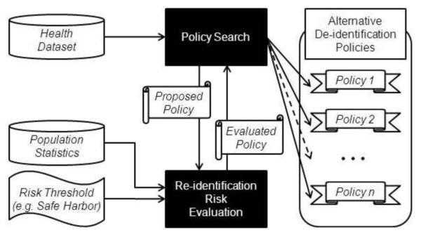
A general architecture of the alternative policy discovery process.

2.2 Policy Representation

Before we can search for alternative de-identification policies, we need a common formalism to relate the HIPAA Safe Harbor policy with alternatives. To clarify what constitutes a de-identification policy, we introduce the following formalism. Without loss of generality, we assume that health data is organized in a table from which explicit identifiers, such as personal names have been removed. The table is comprised of a set of records {T₁, … , T_n}, each of which corresponds to a specific patient and contains a set of attributes A = {A₁, A₂, … , A_m}. Each attribute A_i takes values in a range r(A_i), which contains values that appear in at least one of the records. For instance, the range for the attribute Age could be {0, 1, 2, … , 119}.

The set of attributes A is further partitioned into sets Q and S, such that Q ⋃ S = A and Q ⋂ S = ⊘. Q contains quasi-identifiers, i.e., attributes that may be used to reveal a patients’ identity [8], while S contains all other attributes. In the healthcare domain, Q usually contains patient demographics, such as Age, Zip Code, Race, and Gender, which can be found in public resources with personal identities, such as state voter registration lists [23]. In contrast, S tends to consist of clinical information, such as diagnoses, treatments, or laboratory reports.

For privacy protection purposes, it is often the case that specific values of a quasi-identifier A_i are replaced by more general but semantically consistent values. This process, called generalization, maps one or more values in A_i to the same generalized value. For instance, a generalization of Age could map all values {0, … , 119} in r(Age) to a generalized value 0-119. There may be many different ways to generalize values, but, typically, the allowable generalized values are organized into a generalization hierarchy. Consider for example the hierarchy for Age illustrated in Figure 2. All values {0, 1, 2, … , 119} in r(Age) form the leaves of the hierarchy (due to space constraints, the leaves are shown … in Figure 2). Now, if we map each of these values to a five-year range, we obtain the generalized values 0-4, 5-9, … , 115-119, each of which is the immediate ancestor of all the leaf-level values it replaces (e.g., the values 0, … , 4 have 0-4 as their immediate ancestor). A generalization hierarchy can have more than two levels. For example, if the age value can also be mapped to 10-year intervals, we can extend the hierarchy by assigning two consecutive five-year intervals to each 10-year interval as shown in Figure 2 (e.g., 0-4 and 5-9 will have 0-9 as their immediate ancestor). The topmost level of the hierarchy, however, must contain a single value (*) that represents all values in r(A_i). Given a hierarchy for a quasi-identifier A_i, we define a de-identification policy as a function that maps each value in r(A_i) to a generalized value that is contained in the hierarchy.

Figure 2.

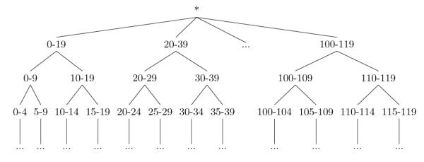
Standard generalization hierarchy for Age.

There are many ways to map specific values to generalized versions according to a hierarchy, which lead to different generalization models. One of these models, called full domain generalization [15], forces all values to be mapped to the same level of the hierarchy. This model has been applied in the healthcare domain [10, 11]; however, it is restrictive and often limits the practical utility of health data unnecessarily [16]. With respect to the HIPAA Privacy Rule, full domain generalization is particularly problematic because it does not efficiently model the Safe Harbor de-identification policy and the range of alternative de-identification policies (e.g., generalized values that are 5-year intervals). Our critique is supported through the following scenario. Consider Figure 2, which illustrates a traditional generalization hierarchy for Age. In this hierarchy, ages are generalized from one- → five- → ten- → twenty-year ranges. While full domain generalization dictates that all values must be assigned to the same level in this hierarchy, HIPAA Safe Harbor policy states that all ages under 89 can be retained intact (i.e., as leaf-value levels in the hierarchy) and ages over 89 must be grouped together into the value 90-119. As such, we cannot accommodate the Safe Harbor policy by generalizing the values using the full domain generalization model within this hierarchy. Rather, to represent this policy we need to amend the hierarchy as depicted in Figure 3. Notice, in the new hierarchy we generalize all values less than 90 to single year values until all ages over 90 reach the Safe Harbor grouping of 90-119. After this point, we can begin the generalization of the ages less than 90 to values with larger age intervals. Yet, while this hierarchy permits the representation of Safe Harbor, notice that it prevents the representation of a policy that specifies all ages should be generalized into equally-sized age intervals!

Figure 3.

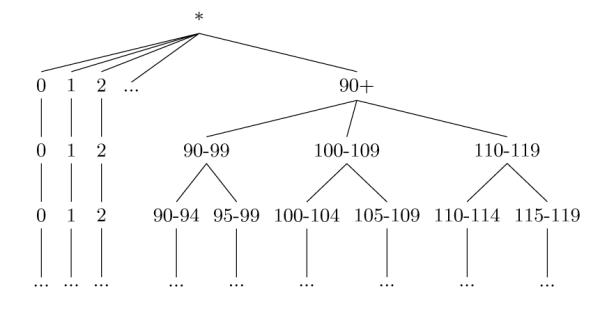
A generalization hierarchy that supports the HIPAA Safe Harbor policy for Age.

A more flexible alternative to full domain generalization is the full subtree generalization model [14]. According to this model, subtrees of values in the hierarchy (i.e., consecutive values such as 0, … , 4) are mapped to a generalized value represented as their closest common ancestor in the hierarchy. When this model is applied to generalize the age values according to the hierarchy of Figure 3, the values 0, … , 4 can be mapped to their closest common ancestor 0-4, while the values 20, … , 39 to their closest common ancestor 20-39. Since this model permits values to map to different levels of a generalization hierarchy, it enables finding a larger number of potentially useful de-identification policies and thus we adopt it in our approach.

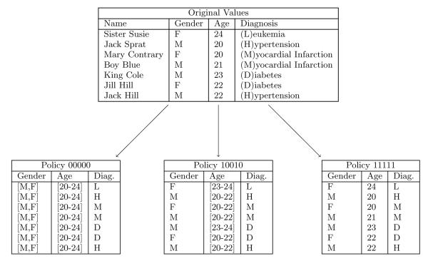
Following [14], we represent a de-identification policy α as a bit-string. For reference purposes, the value of the i^th bit b_i is denoted α[b_i]. The representation for each quasi-identifier A_i consists of n − 1 bits, where n is the number of values in r(A_i). The bits are ordered with respect to the values. When a bit is set to 1, the corresponding value in the range is retained in its most specific form (i.e., a leaf-level value in the hierarchy), and when a bit is set to 0, the corresponding value is generalized with the leaf that is adjacent to it in the hierarchy, if one exists. Consider for example generalizing the age values {0, … , 4} to their closest common ancestor 0-4. The vector corresponding to this generalization is [0,0,0,0]. Policies that model multiple quasi-identifiers concatenate the bit vector for each attribute. Figure 4 illustrates an example dataset and the resulting projections of several different policies.

Figure 4.

Sample dataset and data sharing policies, where Gender and Age are quasi-identifiers.

2.3 Risk Evaluation

A policy indicates how to project the specific values of a dataset into a generalized form. However, a policy does not indicate the degree to which the resulting dataset is vulnerable to re-identification. A policy can, in fact, lead different datasets to different degrees of re-identification risks [3]. Thus, the risk must be computed directly from the records in the dataset.

To determine the re-identification risk for a particular dataset, we compute the expected number of records that can be linked to the correct corresponding identified individuals in the population. We base our re-identification risk metric on the distinguishability metric proposed by Truta and colleagues [24]. Informally, we say that the amount of risk a record contributes is proportional to the number of people the record matches with respect to its quasi-identifier. Formally, we define the re-identification risk for a dataset D to be

$$\text{risk}(D,P)=\sum _{d\in D}{\left(\frac{1}{g\left(d\right)}\right)}^{\gamma },$$ (1)

where g(d) is the frequency of the set of quasi-identifiers of record d ∈ D in the population and γ a positive-valued scaling factor that dictates how much a group size dampens the risk. For this work, we set γ equal to 1, which has a natural interpretation in that the amount of risk a patient record contributes is exactly inversely proportional to their group size. As such, a patient record that is unique in the population contributes a privacy risk of 1, whereas a a record in a group of five contributes a privacy risk of 0.2. This function has range (0, ∣D∣], where ∣D∣ is the size of the dataset D. In practice, this value will often be normalized by the size of the dataset, resulting in a range of (0, 1].

In prior research, such as [24], the group size was computed directly from the dataset. In other words, the group size for a given record would be the frequency of the set of quasi-identifiers of this record in D. This computation is relevant when a quasi-identifier is defined over attributes for which population statistics are unknown. However, this usually leads to a conservative estimate of the group size. In reality, it is often the case that statistics about the population from which the dataset was derived are available, which lead to group sizes that tend to be larger. In particular, in the context of the HIPAA Privacy Rule, the distribution of the combination of demographic attributes in the Safe Harbor policy, such as Age and ZIP Code, as well as other notable features, such as Ethnicity and Gender is made publicly available by the U.S. Census Bureau (e.g., number of 50-year old white males living in a particular ZIP). Thus, we follow the work of [13] and use the Census data to set g_d.

Having defined the risk measure, we prove that it is monotonic in Theorem 2.1. This property is important to using this measure in discovering alternative policies, as we will show in the next section.

Theorem 2.1 (Monotonicity). Let α and β be policies on a generalization lattice. If α is an ancestor of β, then risk(α(D), P) ≤ risk(β(D), P), where risk(a(D), P) is the risk of anonymizing D according to a policy α.

Proof

Let α(d), β(d) be the policy mapped versions of d ∈ D, with corresponding group sizes of g(α(d)), g(β(d)). If is an ancestor of β, then it directly follows that g(α(d)) ≤ g(β(d)). Thus, by Equation 1, we have that risk(α(d), P) ≤ risk(β(d), P). Since this holds true for all records in D, it is guaranteed that risk(α(D), P) ≤ risk(β(D), P).

2.4 Policy Search

The representation of policies as bit vectors enables a natural partial ordering to the space of all policies that can be found using the full subtree generalization model. In particular, the policies can be ordered on a generalization lattice structure. Due to space restrictions, we do not formally present the way such a lattice is constructed, but refer the reader to [15] for details. An example of a lattice is shown in Figure 5. The bottom of the lattice (level 0) corresponds to a policy in which each quasi-identifier is given with full specificity for every possible value. On the other hand, the top of the lattice (level 6) corresponds to a policy in which each quasi-identifier is generalized to the most general level (*) of a hierarchy. Edges between policies on the lattice connect policies which have the smallest possible difference in the way values are generalized. This difference corresponds to two values being generalized differently or a one bit difference in our bit-string representation.

Figure 5.

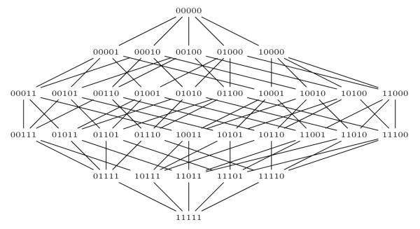
Example lattice for the de-identification policies that can be discovered from the sample dataset in Figure 4.

Armed with a way to represent all possible policies, we will characterize the policies that our approach attempts to discover. First, we define a dominating policy as follows.

Definition 2.1 (Dominating Policy). Given dataset D, a generalization lattice containing policies α and β, and a re-identification risk threshold T, we say that α dominates β if risk(α(D), P) ≤ T and α is a descendant of β.

A dominating policy is therefore a more desirable deidentification solution than the policy it dominates. Furthermore, due to the monotonicity property of our risk measure shown in Theorem 1, we know that the dominating policy will always be a descendant of the dominated one.

Based on the notion of dominating policies, we also define a risk-minimal policy as a policy that is not dominated by any of its descendant policies in the lattice, as explained in Definition 2.2.

Definition 2.2 (Risk-Minimal Policy). Given a dataset D, a generalization lattice, and a re-identification risk threshold T, a policy α is risk-minimal if and only if: (i) risk(α(D), P) ≤ T, and (ii) α is not dominated by any of its descendants in the generalization lattice.

A risk-minimal policy is thus a policy that it is safe according to the risk measure, but none of its descendants is. Note that the set of all the risk-minimal policies for a dataset contains the best alternative policies that can be discovered. However, discovering risk minimal policies is impractical because it requires ordering a combinatorially large number of policies within the same level of a generalization lattice, which is computationally expensive. Assume for example that the policy represented as 00001 in Figure 4 satisfies the risk threshold. This implies that all of its immediate descendants 00011, 00101, 01001, 1001 need to be checked to determine if 00001 is risk-minimal. More generally, for a policy whose bit-string contains z zeros, all z − 1 immediate descendants have to be examined.

To minimize the overhead of discovering alternative policies while still guaranteeing that these policies will be safe, we somewhat relax the properties of a risk-minimal policy by requiring a single descendant of this policy to have an unacceptably large risk. We call such a policy a boundary policy and define it as follows.

Definition 2.3 (Boundary Policy). Given dataset D, a generalization lattice, and re-identification risk threshold T, a policy α is a boundary policy if and only if: (i) risk(α(D), P) ≤ T, and (ii) there exists another policy β, such that β is a descendant of α in the generalization lattice and risk(β(D), P) > T.

Using the lattice-based representation of policies and the above definition, we formally define the problem of discovering alternative policies as explained below.

Problem 2.1 ( Policy Discovery). Given a dataset D, a generalization lattice, and a threshold T, find all boundary policies.

Thus, in this work we attempt to discover boundary policies that are not dominated in the generalization lattice. As our experiments illustrate, this is sufficient to discover a large number of alternative de-identification policies. Before presenting our algorithm to find alternative de-identification policies, called Bisecting Policy Search, we introduce a simple heuristic called Directed Policy Search. The latter heuristic is used as a basis for comparison.

2.4.1 Directed Policy Search

The Directed Policy Search algorithm implements a directed walk on the generalization lattice and is initiated by selecting a random policy in the lattice. If the policy has risk no greater than the threshold, then we walk down the lattice, randomly choosing a child of the current policy, until we find a policy with risk that is above the threshold. When such a policy is reached, we report the parent of the current policy as a boundary policy. If, on the other hand, the initial policy had risk greater than the threshold, we walk up the lattice, randomly choosing a parent of the current policy, until we find a policy that has risk no greater than the threshold. At this point, the current policy is reported as a boundary policy.

Algorithm 1.

Bisecting Policy Search (BPS)

Input: n, number of iterations; T, maximal acceptable risk;  D, dataset for evaluation; P, population statistics de-  fined over the attributes in the quasi-identifier Q

Output: solutions, list of boundary policies

1: solutions ← ∅;

2: for i = 0 to n do

3:    max ← [0, 0, 0, …,0]

4:    min ← [1, 1, 1, …,1]

5:    while levelsBetween(min, max) ≥ 2 do

6:      currentPolicy ← halfwayPoint(min, max)

7:      currentRisk ← risk(policy(D), P)

8:      if currentRisk ≤ T then

9:       max ← currentPolicy

10:      else

11:       min ← currentPolicy

12:      end if

13:     end while

14:     solutions ← solutions ⋃ max

15: end for

16: return solutions

2.4.2 Bisecting Policy Search

We leverage the monotonicity property of risk in the lattice to find boundary policies in a more efficient manner. Specifically, our Bisecting Policy Search (BPS) strategy, shown in Algorithm 1 utilizes a binary search on the lattice. The inputs to the algorithm are the number of iterations n to search for policies, the dataset D to de-identify, the relevant population statistics P, and the maximal level of reidentification risk to be accepted for a policy T (set to the level of risk data anonymized using Safe Harbor incurs in our experiments). The output of the algorithm is a list of boundary policies.

Here, we provide a walkthrough of the search process. In step 1, the set of solutions is initialized to the empty set. The bisecting search is then repeated for the number of iterations specified in the input n. During each search, the variables max and min are initialized to the most general policy and the most specific policies on the lattice, respectively. This is done to provide a bound on the search space that includes all possible policies. The search space is repeatedly halved by selecting a policy that is halfway between min and max. This is called the current policy (currentPolicy). The reidentification risk for the current policy is then computed (Step 7) using the modified version of Equation 1, which we refer to as currentRisk. The risk of the policy determines its acceptability and thus the portion of the lattice which can be eliminated from the search. The acceptability is determined by a simple comparison to evaluate if its risk is no greater the risk threshold (Step 8).

Each step on the lattice halves the search space, eventually resulting in a convergence of min and max. An iteration of the search halts when min and max are on adjacent levels. To determine if two policies are on adjacent levels, we apply the levelsBetween function (Step 5), which counts the Hamming distance between policies α and β:

$$\text{levelsBetween}(\alpha ,\beta )=\mid \alpha \oplus \beta \mid$$

where ⊕ is the bitwise XOR. This essentially returns the number of levels that exist between the two policies. The policy found as a result of the search is added to the set of solutions.

During the search process, it is possible to choose the halfway point completely at random by finding the bit positions where the policies disagree and flipping half of the. However, to orient the system toward generating a diversity of de-identification solutions, we instead choose from among these options using a probability distribution derived from a set of weights. We use two sets of weights in this computation. The first weight is based on the size of the range of the attribute that each bit in position i, or b_i represents.

$$w_{\text{sizeOfField}}\left(b_i\right)=\mid r\left(A_i\right)\mid -1$$

This weighting scheme prevents us from falling too frequently into policies which generalize small domains. For example, the attribute of Gender only has two values, and the impact of generalizing the two together is very large. By choosing it less often, we can explore a wider variety of solutions.

The second weight is based on previous solutions. The weight for a bit is proportional to the number of times that the bit has been set in previous solutions.

$$w_{\text{previousSolutions}}\left(b_i\right)=\sum _{s\in \text{solutions}}s\left[b_i\right]+1$$

This weighting also has the effect of finding more diverse solutions. If a particular bit has been set in many previous solutions, we reduce the probability of choosing it in the future.

We combine the weights through an additive formula:

$$w\left(b_i\right)=w_{\text{sizeOfField}}\left(b_i\right)+w_{\text{previousSolutions}}\left(b_i\right)$$

Now, imagine there are x policies to choose from, then the probability that we choose the available policy with the change in bit i is $w\left(b_i\right)∕{\Sigma }_{j=0}^{x}w\left(b_j\right)$.

Let us return to the example dataset in Figure 4 to illustrate an example. Table 1 shows one iteration of the BPS algorithm which would result in a report that policy 10010 is a boundary policy. The resulting projection of the example dataset on this policy is in Figure 4.

Table 1.

One iteration of the BPS algorithm.

Step	Upper Bound	Lower Bound	Current Policy	Policy Acceptable?
1	00000	11111	10010	Yes
2	10010	11111	10110	No
3	10010	10110	None	None

3. EXPERIMENTS

3.1 Materials

For this study, we selected several datasets to evaluate the proposed de-identification policy discovery method. The first dataset corresponds to the demographics of a set of 2984 patients from the Vanderbilt University Medical Center, 12 of which have age 90 or greater. This dataset is of interest because the patient records are currently being used for an NIH-sponsored genome-wide association study on native electrical conduction within the ventricles of the heart (further details are available in [18]). The second dataset is based on the publicly available Adult corpus, consisting of 32,561 records, 43 of which have age 90 or greater, which has been used to evaluate numerous data anonymization algorithms [14, 15, 16]. We refer to these datasets as the Van and Adult datasets, respectively. For demonstration purposes, we explore the space of policies in the combined domain of {Gender, Race, Age}. The Race domain differs for the two datasets. In Van, Race is a 7-valued attribute, while in Adult, Race is a 5-valued attribute.

For the purposes of this study, we make the assumption that the U.S. state of residence for all records in both datasets was Tennessee. This assumption is used with reference to the population statistics. We use population statistics derived from the 2000 U.S. Census, Tables PCT12 A-G, available from American Fact Finder. These tables detail the number of people of each gender, by age, in a particular geographic division, each table representing one of the Census’s seven race classifications.

All experiments were run on a machine with an Intel Core 2 Duo processor at 2.00 GHz with 2 GB of RAM.

3.2 Results

The evaluation is organized into two subsections on efficiency and effectiveness.

3.2.1 Efficiency

In the first set of experiments we investigated the efficiency of the approach. We begin the assessment with an amortized analysis to demonstrate the benefits of the BPS approach. Table 2 summarizes the runtime of the BPS and Directed search algorithms. Both algorithms were run for 100 iterations (i.e., they discovered 100 boundary nodes in the lattice). The table reports the mean and standard deviation of the search time per iteration. For the Van dataset, the mean search time for the BPS approach required 4 seconds on average, whereas the Directed approach required over ten times as much time at 47 seconds. A t-test yielded that the BPS approach was faster than Directed by a statistically significant margin at the 95% confidence level. For the Adult dataset, the BPS approach was once again faster by almost ten times (statistically significant at the 95% confidence level); it required 16 seconds on average, whereas the Directed approach required 109.

Table 2.

Summarized runtime analysis. Time per iteration of search for boundary solution.

METRIC	Directed		BPS
	Van	Adult	Van	Adult
Average (seconds)	47.52	109.53	4.01	16.36
St. Dev.	2.03	8.94	1.85	2.00

To illustrate the real world applicability, we move beyond summary statistics and illustrate how long the policy discovery process requires across iterations of the algorithm. Figure 6 provides a visualization of the cumulative search time as a function of the number of iterations (i.e., at the x^th iteration, this graph reports the total time to complete the discovery of x boundary policies). Notice that the policy discovery process appears to follow a linear trend for both search algorithms and datasets.

Figure 6.

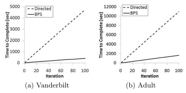
Analysis of policy search runtime for the datasets.

This is interesting because we implemented the search algorithms in a manner that retains the re-identification risk results of each alternative policy found during the execution of the algorithm. It was expected that this would lessen the quantity of time allocated to the search process over time. We performed an autoregressive analysis to determine if the runtime at iteration x − 1 predicted the runtime at iteration x, but observed only a weak correlation. As an example, Figure 7 illustrates that for the BPS algorithm with the Van dataset, a logarithmic trend characterizes only 16% of the variance in the system. Thus, while we recognize that 100 may be a relatively small number of iterations, it appears that the number of paths in the lattice that result in reidentification risk less than Safe Harbor is extremely large, such that a heuristic-based approach for policy discovery is justified.

Figure 7.

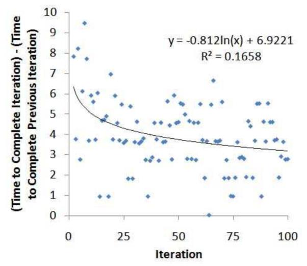
Autoregressive analysis of policy discovery time of iteration x on iteration x − 1 for the BPS algorithm with the Van dataset.

3.2.2 Effectiveness

In the second set of experiments, we evaluate the quality of solutions discovered by the policy search algorithms. As mentioned earlier, the policy discovery algorithm completes an iteration when a node satisfies the boundary condition. However, it is possible, that in a subsequent iteration of the algorithm, a dominating solution will be discovered. The BPS algorithm incorporates a heuristic to bias starting nodes in an iteration to prevent domination whereas the Directed algorithm did not. To evaluate the effectiveness of this heuristic, we computed how many of the boundary nodes discovered in 100 iterations of the algorithm were non-dominating. If the solutions are not on the same path in the generalization lattice, then 100 polices will be non-dominating, but if all are on the same path only one would be non-dominating. Figure 8 illustrates how many of the x iterations were found to be non-dominating. For a detailed analysis, Figure 8 illustrates the results for the Van dataset. Here it can be seen that for the first 25 runs, both the BPS and Directed algorithm are competitive and discover zero non-dominating solutions. After this point though, the BPS algorithm outperforms the Directed algorithm at an increasing rate. By the 100^th iteration, the BPS algorithm discovered 95 non-dominating policies, whereas the Directed algorithm discovered only 83 (i.e., 13% less).

Figure 8.

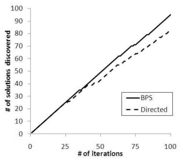
Effectiveness plots at the iteration level for the Vanderbilt dataset.

It is also important to recognize that there is a difference in the number of nodes searched per iteration. Recall, the Directed algorithm uses a walk from an initial randomly selected node to the boundary policy, whereas the BPS algorithm uses a more intelligent skip-based approach. As a result, it is expected that the BPS algorithm discovers alternative de-identification policies with less nodes searched than the Directed algorithm.

Figure 9 illustrates that BPS discovers solutions in a fraction of the nodes searched than Directed. This finding was implied in the runtime analysis, but this figure clearly illustrates that at the completion of the policy discovery process, for the Adult dataset BPS has searched only 670 nodes in the lattice, whereas Directed has searched 5140 as shown in Figure 9(b). A similar result was observed for the Vanderbilt dataset (Figure 9(a)).

Figure 9.

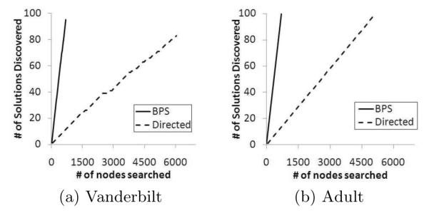
Effectiveness plots at the node search level.

3.3 Example Alternatives

Table 3 provides examples of the types of alterative (non-dominated) policies that were discovered for the Van dataset. By manual inspection, the exemplars appear to represent different types of policies. We represent these policies by the generalizations required for each attribute. Only the values which are generalized together are displayed. All other values are kept in their most specific form. For context, the first row shows the Safe Harbor policy. The first alterative corresponds to the situation in which the gender attribute is completely generalized while retaining full specificity in the ages of the patients. Recall, there were 12 patients over the age of 89, which Safe Harbor prohibits disclosing in detail. The second alternative shows that gender can be retained, but the value of Asian must be generalized with the “Other” race value. The third alternative shows that both gender and race can be retained in their most specific form when the ages of 52 and 53 are grouped into a single 52-53 value.

Table 3.

Examples of discovered alternative de-identification policies for the Vanderbilt dataset.

	Generalizations
Policy	Gender	Race	Age	Risk
Safe Harbor	∅	∅	[90-120]	0.90917
Alt. 1	[M,F]	∅	∅	0.47628
Alt. 2	∅	[Asian, Other]	∅	0.85703
Alt. 3	∅	∅	[52-53]	0.87498

4. DISCUSSION

In this work, we utilized a formalism that allows us to compare the HIPAA Safe Harbor and alternative de-identification policies with the aim of finding a process to satisfy the Expert Determination standard. This formalism enables the use of full-subtree generalization to construct a lattice with properties that enable efficient searching. We evaluated our search strategy and the results illustrate that it performs significantly faster than a directed walk. It is important to recognize that many policies were found that have reidentification risk that is equal (or lower) than Safe Harbor for both of the datasets we examined. Moreover, these policies were varied in the portions of the attributes in which generalizations occurred. This suggests that even for epidemiologists and researchers in gerontology there may be policies which will keep needed information intact while providing privacy protection. Though this work focused on certain demographics, it could easily be extended to include other attributes, such as ZIP code. This would provide a rich, detailed field for comparison and further highlight the advantages of a bisecting strategy. Such detail is not available for the Adult dataset, but it could be simulated using available population statistics from the U.S. Census.

There are several limitations of the work that we wish to mention to spur future research. First, while we prove that such alternatives exist, it remains to the healthcare community to decide whether such a system will be adopted. We believe that our approach is interpretable, such that it can be presented to Institutional Review Boards, and qualify under the Expert Determination as a “documented method”.

Second, one of the hazards with looking at a large search space to find possible solutions, without some kind of a priori assumptions about which solutions are better, is the potential for a glut of information provided to the end user. While we maintain that it should be up to the health data manager to determine which solutions work for their dataset, we believe that an interesting research area is in determining how possible de-identification solutions could be presented to a data manager to support their decisions in a comprehensible, user-friendly manner. One particular direction that is promising is in the application of clustering. If the deidentification solutions, as reported by the algorithm, can be grouped into clusters, the data manager could be supplied with examples from each cluster to assist in reasoning about which are the most appropriate for their dataset. Along this line of research, it may be possible to combine the search algorithm from this paper with post-processing into a single step, as has been achieved in genetic algorithms [21]. Such algorithms typically represent solutions with bit-strings and employ powerful strategies to retain the most ”desired” solutions. However, to employ these algorithms, we need to accurately measure the “goodness” of solutions, which is not straightforward in the healthcare domain.

Third, there were certain assumptions we made about reidentification risk which should be considered. Notably, the risk metric we applied assumes an attacker is equally interested in all records, which may not always be the case. Additionally, the risk measure considers “identity” disclosure; i.e., the linking of a patient’s identity to their record, which is a common threat in the healthcare domain. Extensions with alternative protection models, such as those that prevent the association of an individual to their sensitive information (e.g., a diagnosis code) are still possible and the subject of future research.

5. RELATED WORK

The problem of re-identification has attracted significant interest and is typically mitigated by modifying data in a way that reduces the re-identification risk to an acceptable level. Data modification can be performed by perturbation methods, including additive noise, data swapping, and synthetic data generation (see [1, 25] for surveys). While these methods preserve certain aggregate statistics, they generate data that does not correspond to real patients (e.g., they could swap the age of a 90-year old with that of a 20-year old, affecting the validity of a geriatric study). This implies the records can no longer be analyzed individually, which is crucial in a number of healthcare applications, such as epidemiological studies [20].

Thus, our approach does not use perturbation methods to discover policies, but employs generalization [23], a technique that replaces values in quasi-identifiers with others that are more general but semantically consistent. Generalized records are truthful and can be examined individually. For example, when the age value 90 for patient is replaced by the generalized value 90-99, this patient’s actual age can still be inferred from the generalized one. Generalization can be performed using a number of different models [15]. These include full domain generalization, a model in which all the values of a quasi-identifier are mapped to generalized values that lie at the same level of a given hierarchy, and full subtree generalization, a model in which only subtrees of values in the hierarchy of a quasi-identifier are replaced by generalized values in a way that the path from each original value to the root in the hierarchy contains no more than one generalized value. We have adopted the full subtree generalization model in our approach for the reasons discussed in Section 2.2.

Generalization plays a central role in ensuring that data can be safely released according to a number of different privacy principles. Perhaps the most well-established of these principles is k-anonymity [23], which requires each record in the released data to have the same generalized values with at least other k-1 records over the quasi-identifiers, which limits the probability of re-identifying a patient to $\frac{1}{k}$. Subsequent methods strengthen the protection provided by this principle by imposing further restrictions on the frequency of attributes which are not treated as quasi-identifiers (e.g, a patient’s diagnosis). Examples of these principles include l-diversity [19] and t-closeness [17]. We note that our policy discovery approach is independent of the underlying privacy principle and can be modified to support all of these principles. In fact, since the measures of [19] and [17] are all monotonic, we simply need to check whether a policy satisfies one of these principles instead of having an acceptable level of risk as we currently do. A complete treatment of this issue is, however, a part of our future work.

6. CONCLUSIONS

Regulations, such as the HIPAA Privacy Rule, permit the dissemination of patient data if it meets a de-identification standard. Currently, most organizations de-identify health data by adhering to the Safe Harbor policy, which is easy to apply, but limits the data utility. In this paper, we proposed a process to satisfy a de-identification alternative known as Expert Determination, which can facilitate more flexible disclosure policies. Our approach uses Safe Harbor to set a threshold of re-identification risk admissible in a shared dataset, and then explores the space of alternative de-identification policies in an efficient and effective manner to find polices with risk no greater than the threshold. Furthermore, our approach is generalizable in that it can be used with several other privacy principles and policies. Our experimental evaluation utilized both patient records and census data to demonstrate that there are many potential de-identification alternatives to Safe Harbor that can satisfy the Expert Determination standard. In future research, we anticipate extending this research to assist health data managers in reasoning about which alternatives are the best option for their particular dataset.

APPENDIX A. SAFE HARBOR POLICY

Section §164.514 of the HIPAA Privacy Rule provides the de-identification standard for health information. Following this standard, health information is not individually identifiable if it does not identify the individual or if the covered entity has no reasonable basis to believe it can be used to identify the individual. The Safe Harbor policy specifies that a list of “identifiers of the individual or of relatives, employers, or household members of the individual, are removed”. For reference, Table 4 provides the list.

Table 4.

Safe Harbor blacklist of the HIPAA Privacy Rule.

1. Names
2. All geographic subdivisions smaller than a state, includ- ing street address, city, county, precinct, ZIP code, and their equivalent geocodes, except for the initial three digits of the ZIP code if, according to the current publicly available data from the Bureau of the Census: The geographic unit formed by combining all ZIP codeswith the same three initial digits contains more than 20,000 people; and The initial three digits of a ZIP code for all such geographic units containing 20,000 or fewer people is changed to 000
3. All elements of dates (except year) for dates that are directly related to an individual, including birth date, ad- mission date, discharge date, death date, and all ages over 89 and all dates (including year) indicative of such age, ex- cept that such ages and elements may be aggregated into a single category of age 90 or older
4. Telephone numbers	5. Fax numbers
6. Email addresses	7. Social security numbers
8. Medical record numbers	9. Health plan beneficiary numbers
10. Account numbers	11. Certificate / license num -bers
12. Vehicle identifiers and se- rial numbers, including license plate numbers	13. Device identifiers and se- rial numbers
14. Web Universal Resource Locators (URLs)	15. Internet Protocol (IP) ad- dresses
16. Biometric identifiers, in- cluding finger and voice prints	17. Full-face photographs and any comparable images
18. Any other unique, identifying number, characteristic, or code