Genetic and Molecular Network Analysis of Behavior

Abstract

This chapter provides an introduction into the genetic control and analysis of behavioral variation using powerful online resources. We introduce you to the new field of systems genetics using "case studies" drawn from the world of behavioral genetics that exploit populations of genetically diverse lines of mice. These lines differ very widely in patterns of gene and protein expression in the brain and in patterns of behavior. In this chapter we address the following set of related questions: (1) Can we combine massive genomic data sets with large aggregates of precise quantitative data on behavior? (2) Can we map causal relations between gene variants and behavioral differences? (3) Can we simultaneously use these highly coherent data sets to understand more about the underlying molecular and cellular basis of behavior?

Introduction

The theme of this chapter is how best to go about discovering and testing for associations between differences in DNA sequence and behavioral variation. In this particular instance, we introduce you to powerful bioinformatic and genetic tools and techniques that are still "under-the-radar." There is a good chance that you will be able to apply these new techniques to specific problems, even while you read. If you have a computer with an Internet connection—so much the better, and you can read and work along at the same time. This short review and primer will take you on a tour of a web site called GeneNetwork that embeds many large data sets that are relevant to studies of behavioral variation. GeneNetwork is an unusual site because it contains a coherent "universe" of data, as well as many powerful analytic tools. You could think of this site as a massive collection of linked Excel spreadsheets and macro commands—some spreadsheets with extensive behavioral data for dozens to hundreds of cases (primarily mice and rats), some spreadsheets with genotypes for the same cases, and some spreadsheets with data on gene expression for dozens of brain regions (again for the same cases). The great majority of behavioral data, along with a simple “controlled vocabularies” have been extracted and curated by the GeneNetwork team from the published literature. Data are usually hyperlinked to the most relevant references, although you may also encounter some unpublished and some pre-published data.

With some persistence, you will be able to (1) find appropriate behavioral data, (2) test specific hypotheses about gene-to-phenotype relations ("are mice with bigger brains or bigger hippocampii smarter in a water maze task?"), or (3) generate "de novo" hypotheses using single concepts or single genes as your seeds. Our only expectation is that you are interested in behavioral variation and in ways to exploit bioinformatic resources and methods to dissect and (we hope) reassemble and model behavior. You do not need to be a statistician or geneticist to use these tools.

In order to use GeneNetwork, we have to start with some ground rules and assumptions. The first is that behavioral traits must vary significantly. This is a chapter about behavioral variation with an equal emphasis on both words. If a behavior is a "fixed action pattern" that is truly invariant across some population of humans, mice, rats, or drosophila, then it is off-topic from the point of view of this chapter and also off-topic for most genetics analyses. Genetics is the study of variation—heritable or not. Genetics is not the study of genes, although of course, it does include the study of genes. Variation may be measured on a qualitative scale (green versus red), a rank or ordinal scale (high, medium, low), or a standard quantitative scale (linear, logarithmic, z scores, etc.). The upshot is that when we talk about behavior in this chapter we really mean variation in behavior measured on a defined scale. All of the behavioral data in GeneNetwork is about variation across organism populations or families of individuals.

The second and closely linked ground rule: discard any tendency toward what is sometimes called “typological thinking”. This happens daily at conferences and in papers. Data on a set of 10 Sprague-Dawley juvenile male rats becomes "the rat" and data on a set of 10 C57BL/6J mice becomes "the mouse". Mouse, rat, and human are handy nouns, but these nouns cannot be reified into single types without serious risk of being wrong. All rats are white and all mice are black is a valid conclusion if we consider Sprague-Dawley and C57BL/6J as representatives of their species. We can profit from something somewhat analogous to Heisenberg's Uncertainty Principle to remind us that "types" are fuzzy around the edges, and that there may be as many exceptions as there are rules. The reason to emphasize this point is that behavioral traits are variably variable within and between species. This variation is an experimental treasure trove rather than a technical nuisance.

The third critical assumption is that differences in DNA sequence cause differences in phenotypes, including behavior; not the other way around. Thinking back more than a hundred years to the Lamarkian controversy of the inheritance of acquired traits (Bowler, 1992), this would seem to be a fact on solid ground, but everyone loves an argument. For the purpose of this review, we ask you to accept the central dogma of behavioral genetics: DNA variants produce RNA variants which in turn produce protein variants, and after many intervening steps (our collective black box), these DNA variants contribute to variation in phenotypes. All behavioral traits are therefore built up using multiple gene products, complex molecular cascades, and tiers of different types of cellular and environmental interactions. A fraction of the variation in almost all behavioral traits can be "associated" back to gene variants and chromosomal locations. This is what we mean when we say that we have genetically "mapped a trait". The word "association" is unfortunately often used in this context, but association in this sense is much more than just a bland statistical association. This is a causal and even mechanistic association. When a study asserts that a particular genetic difference is associated with behavioral differences such as severity of choreiform movements (Huntington disease) then this is an assertion that a cause has been located in the genome. The statistical strength of that causal assertion is measured using a p value (small values are better and mean that the null hypothesis has been rejected) or a logarithm of the odds ratio—a so-called LOD score (big values indicated strong likelihood that the null hypothesis has been rejected and that some genetic causality has been discovered). We may not yet know the specific cause or how this cause operates on behavior, but at least we have an approximate chromosomal location for one or more causal sequence variants. This is why we call this type of genetic discovery a "locus" or, in plural form, "loci." Discard the idea that genetic associations and loci are mere associations—they are assertions of genetic causality with perhaps mysterious mechanistic causes. If a trait "maps" to a locus then that is where the DNA sequence variant (or variants) is fixed. They cannot environmentally or epigenetically wiggle off of the genome or to some other distant part of the genome.

The fourth and final ground rule: Many gene differences and many environmental factors contribute to variation in behavior and we need a rule or general experimental paradigm to understand the connections. The rule is pretty simple: analysis first, integration and validation second. The first analytic step usually involves reducing behavioral complexity. This may seem like throwing the baby out with the bathwater, but we have to start somewhere and we may as well start with simple relations, simple models, and simple hypotheses, and build up from these atoms of behavior to more holistic networks. The next section introduces a process known as genetic dissection, and in our specific case we will analyze the genetic basis of variation in learning and memory. This is called "genetic" dissection for the simple reason that we are attempting to dissect a set of DNA sequence variants and loci that contribute to variation in the trait. The first results of a genetic dissection are lists of quantitative trait loci (QTLs) and candidate genes and variants. The goal is certainly not to stop with QTLs. We would like to get back to the biology of the behavior in question and we can do so by exploiting our loci and heritable variation to do this efficiently.

Step 1: Genetic Dissection of Behavioral Variation using GeneNetwork

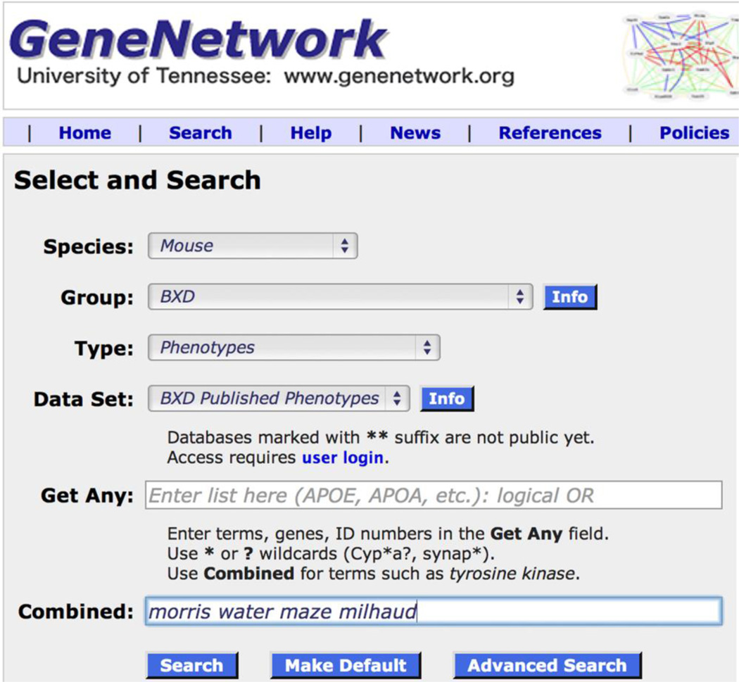
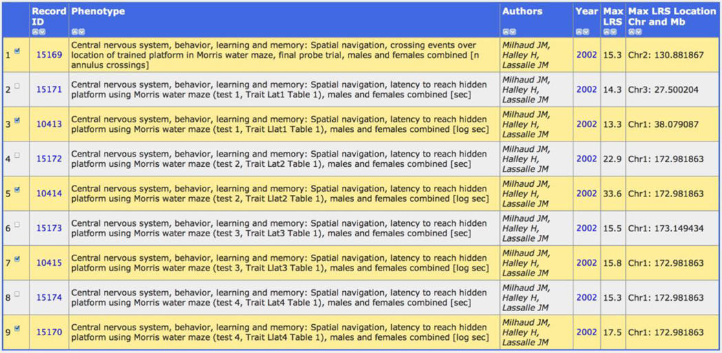
We will work through a simple example of how to use GeneNetwork to analyze differences in a well known learning and memory task called the Morris water maze. We will use a set of nine related traits published by Milhaud, Halley and Lassalle (2002) that can all be accessed in GeneNetwork. Figure 1 provides you with a quick example of how to get these data. If you want to follow along, link to http://www.genenetwork.org. Change the default Type to read Phenotypes. Then type in a string of search terms. In Figure 1, the terms were water maze morris and milhaud, and they were entered into the Combined search field. If you click on the Search button, you will retrieve all nine traits (Figure 2).

Figure 1.

The Search page on GeneNetwork being used to find published behavioral data on the water maze task from a paper by Milhaud and colleagues.

Figure 2.

Behavioral data from a learning and memory task (water maze). Each description starts with the same general terms ("Central nervous system, behavior... " and then provides more detail on the actual assay, cases, and units. Four of these nine traits (clear background) are times it takes a mouse in seconds to find a hidden platform in a small pool of water. Traits with yellow background are log transformed version of the same data. The top entry is the so-called final "probe" trial result that evaluates the strain's ability to recall platform location even after the platform is removed. Animals swim over the expected location of the platform even in its absence.

The water maze task is used to test learning and memory performance, but like many tests, the results are influenced by motor coordination, sensory capabilities, diurnal rhythm, responses to stress, etc. The actual measurement units are the times in seconds or log seconds that it takes an animal to swim from a variable point of entry in a small pool of water to a hidden “escape” platform that is located in a fixed position in the pool. Animals have been familiarized with the task in pretest trials and they know in general that it would be in their best interest to find the hidden platform. This is a test of orientation, recall of the platform location, motivation, and speed of swimming. You can see that our interpretation for this simple test is already rife with anthropomorphisms about the thoughts, moods, and motivations of rodents, but at least we have an idea about what we are measuring operationally and what we think the data might signify. The great thing about having access to the data in Table 1 in GeneNetwork is that we can let these numbers speak for themselves. Do the traits map strongly to any chromosomal location? If so, what fraction of the variance in the trait can be causally linked to the location(s)? Does performance on this task, whatever it may be measuring, covary with hippocampal size or body weight? To what extent does the speed of finding the platform during the learning phase of the study correspond to the persistence with which the strains search for the missing platform?

To answer some of these questions we can start by selecting a single trait and clicking on its Record ID. All available data for this record is displayed in the Trait Data and Analysis form. The trait measurement for each of the 28 genotypes of mice is shown in the Review and Edit Data section. All of these genotypes or strains are members of the B-by-D or, simply, the BXD family. The B-type mother is the darkly pigmented (BL = black) C57BL/6J inbred strain of mouse whereas the D-type father is the Dilute Beige Agouti or DBA/2J inbred strain. Every one of the progeny genotypes is itself a fully inbred strain and each locus in these progeny is either D/D or B/B. If you were to scan along a single chromosome in these progeny, you would notice alternating long sections that are all B/B genotypes and then a switch to all D/D genotypes. These long blocks of genotypes inherited from one parent or the other are called haplotypes. Family members differ in much the same way that human siblings differ. However, in this particular case we have 26 large sets of identical twins in a single family, with the added quirk that identical twins can be either sex. The ability to resample each genotype a large number of times (12 times in this case) means that experimentalists and statisticians can evaluate and improve the technical precision of measurements by resampling or censoring data. This unique feature also makes it practical to systematically change the environment and assess how the same set of genotypes respond alike or differently. Despite the fact that the study by Milhaud is now over a decade old, we can combine these valuable behavioral measures with complementary and newer data on hippocampal neuroanatomy (Peirce et al., 2003), hippocampal electrophysiology (Rietman et al., 2012), and hippocampal gene expression (Overall et al., 2009), and even adult neurogenesis in the dentate gyrus (Kempermann et al., 2006); all using the same genotypes of mice.

To foreshadow the last section of this chapter, it is this ability to mix, match, and combine phenotype data for populations of genotypes from many labs that gives the BXD family and other so-called genetic reference populations such as the Collaborative Cross their remarkable power in behavioral neuroscience. If your first question is "Won't environmental differences among studies disrupt the comparison?" then you are on the right track. Environmental differences will tend to systematically lower correlations between studies (error terms are rarely shared) leading to a conservative bias in correlation coefficients. It is also possible to rephrase this as an excellent opportunity to test the impact of environment factors on behavior. If two studies conducted more than a decade apart using the same genotypes but different individuals raised in different environments agree closely as judged by a simple correlation coefficient between measurement across all 28 genotypes, then this tells you something important about that phenotype—namely that it is robust to numerous largely undefined environmental differences among laboratories and cohorts. It also tells you that you are likely to be dealing with a highly heritable trait that will be a good target for genetic dissection and QTL mapping.

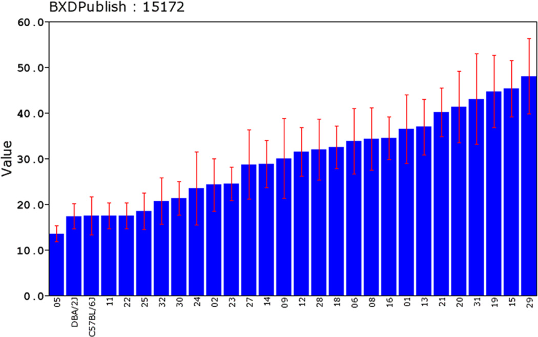
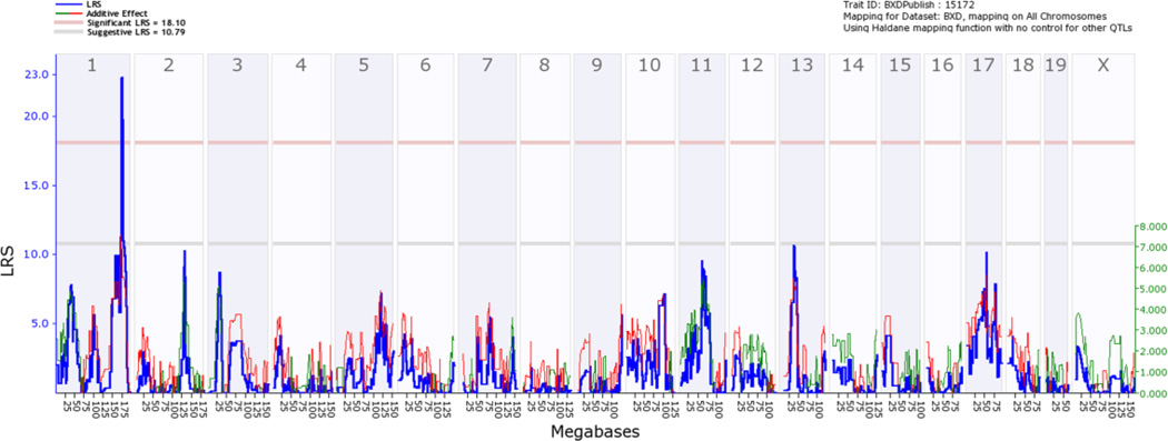
The initial step in genetic dissection is simple—we compute correlations between variation in the phenotype (seconds to reach the platform, see Figure 3 or click on Basic Statistics, Bar Graph) across all of 26 or more progeny BXD strains and their inheritance of either the B or D genotypes (genotypes are coded as −1 and +1). These animals are inbred homozygotes, so they actually have either B/B or D/D genotypes, but we can keep this simple and refer to B/B and D/D as the B and the D genotypes (or alleles). There are just over 5 million known sequence differences between B and D parents, but all we need is a representative subset of about 3000 of these polymorphic chromosomal markers to scan across the collection of all 19 mouse autosomes (and the X chromosome) at a fairly tight spacing—one marker every million base pairs of DNA, or roughly one marker at a spacing of every seven protein-coding genes. The resulting table of correlations and associated p values is unwieldy, but we can convert these data into a smoothed function of p values or the nearly equivalent LOD or likelihood ratio scores (LRS) across the genome. To do this, expand the Mapping Tools section and click on the Compute button under the Interval tab. This gives rise to QTL maps for the whole genome (Figure 4) and for a 20 megabase (Mb) section of chromosome (Chr) 1 (Figure 5).

Figure 3.

A bar chart of the time in seconds (± SEM) that different genotypes of mice take to find the hidden platform on their second test trial in a Morris water maze task. BXD5 (05 in the chart, far left) is fast and well directed to this platform with a time of 13.5 ± 1.7 sec. In contrast, BXD29 (29) is clearly a water-loving wanderer with a time of 48 ± 8 sec. Two key points here: (1) genotype is a significant predictor of time. The raw heritability estimates for these traits are in the neighborhood of 20–30%. (2) The two parental strains have very similar values for this and almost all other traits, but the progeny BXD strains are highly variable. This is because the task is influenced by multiple gene variants that can have counterbalancing effects in parental strains but that segregate freely among the progeny. Trait expression is not controlled by a single Mendelian-type gene variant. This type of chart can be viewed for every trait in GeneNetwork by clicking on the Record ID to navigate to the Trait Data and Analysis page. From this page expand the Basic Statistics section and select Bar Graph (by rank).

Figure 4.

Whole genome map (or scan) for causal linkage between sequence differences and water maze latency (2nd training trial). The x-axis represents chromosome number and megabase location—from Chr 1 to the left to Chr X to the right. The blue function and the left y-axis plot the likelihood ratio statistic (4.6 times the LOD score) of linkage. The pink and grey horizontal lines at values of about 18 and 11 are approximate threshold values (significant and suggestive, respectively) used to establish that a peak is significant given the many thousands of statistical tests involved in a whole genome scan.

Figure 5.

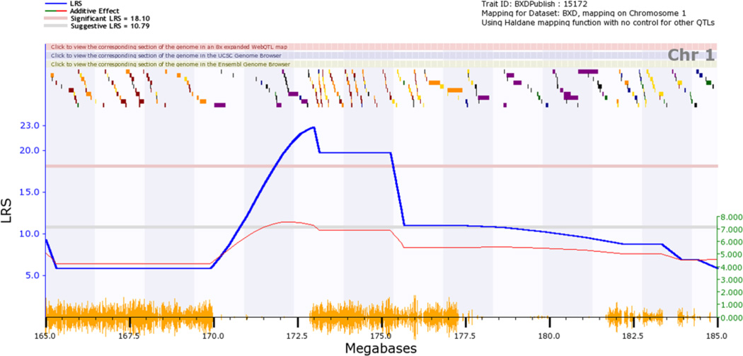
Map of the genetic location on Chr 1 that modulates performance on the water maze task. This is a zoomed version of Fig. 4 that can be generated by clicking on the number at the top of the graph to get a Chr 1-specific QTL map and then by clicking on the red track at the top of the Chr 1 map to zoom in on the targeted Mb region. The locations of individual genes (colored blocks along the top) are superimposed above the LRS score in blue. The thin red line indicates the average effect of switching out a D allele for a B allele. In this case, this so-called additive effect increase the time spent searching for the platform by about 7 seconds per allele (right y-axis). The orange hash on the x-axis highlights the numerical density of sequence differences between the two parental strains. Two large regions are highly diverse and two large regions are very similar between parents.

Let's pause here and summarize. This has already been a successful genetic dissection. We have recomputed and confirmed using much better new genotype data (Shifman et al., 2006) that Milhaud, Halley, and Lassalle discovered a strong QTL that maps to distal Chr 1 for this particular trait and for most of the related data for different days. The correlation between time required to swim to the platform and the single best SNP marker (rs8242852) is 0.78, with an R² of just over ~0.5. About 50% of the genetic variability in the time that it takes members of this family to reach the platform is caused by one or more sequence variants on Chr 1 at 172 to175 Mb. This is an important locus and the underlying sequence variants need to be defined more precisely.

While no one has revisited the water maze paradigm using the much-enlarged BXD family—there are now about 150 members in this clan rather than just 28—we do know that there are strong candidates in the aforementioned region (reviewed in Mozhui et al., 2008). The best is Atp1a2 (Boughter et al., 2012)—a sodium/potassium ion pump that contains over 300 non-coding variants, some of which definitely modulate its expression in brain (higher in strains that inherit the D allele, probably because of a variant in processing of the 3' untranslated region of the mRNA). The genetic and functional linkage of this gene with central pattern generation is unequivocal (Onimaru et al., 2007; Boughter et al., 2012). In humans, mutations in this gene cause migraines. It is possible, even likely, that the linkage to the Atp1a2 region is really more a matter of swimming speed and associated variability of the central pattern generator. Milhaud and colleagues, made this same point and showed that their final "probe" trial trait for memory (numbers of crossing over the missing platform, see GeneNetwork Trait 15169) does not map to Chr 1, but maps to Chr 2 near Adra1d (the alpha 1d adrenergic receptor at 131.4 Mb) and to Chr 5 in the region of Nos1 (neuronal nitric oxide synthase 1) between 116 and 126 Mb. Not nearly as much is known about candidate genes in these two regions as is the case of distal Chr 1. However, Nos1 is a strong candidate that is polymorphic in the BXD family and was independently highlighted by Krebs and colleagues (2011) as a possible modulator of adult hippocampal neurogenesis.

To really resolve questions about what aspects of these traits we are able to map to the genome it would be helpful to have explicit data on swimming speeds for the BXD family. More and better data on spatial memory tasks, such as a radial arm maze task, would also be extremely helpful. Kempermann and Gage (2002) generated data on swimming speed (Trait 10814) that confirm the expectation that we are dealing with at least two phenomena. They found that the correlation between swimming speed is highest (r = 0.8) with the memory data for the training trials (e.g, 10414) and lowest (r = 0.4) for the final memory trial (10814). This supports the idea that time to reach the platform is partly associated with variation in the motor pattern generator. Slow swimmers with the B allele also have a slow licking rate, and lower expression of Atp1a2. The second component represented by the memory "probe" trial is more closely tied to spatial memory and maps to different chromosomes. This illustrates what we mean by the process of genetic dissection of a behavioral trait—or a behavioral complex—and this also highlights the need to let the numbers represent the behaviors that are being measured. Laughlin and colleagues (2011) used this same genetic method to effectively dissect reversal learning in the BXD family using an operant protocol, and were able to highlight a very small number of candidate genes, one of which controls a key aspect of behavioral flexibility.

In the next section, we will go beyond mapping and genetic dissection to study patterns of correlation and covariation among behavioral traits and other higher levels of brain organization. We can test which neuroanatomical, electrophysiological, or behavioral traits covary (or don't) with performance on the water maze but with only modest success. The main limitation has to do with getting the right balance between the complexity of a model of behavior and the sample size of the population needed to critically test that model. While genetic dissection can work with a sample size of 20 to 30 (provided the data are of exemplary quality), a test of a simple model (Shipley, 2002; Li et al., 2006) will require a sample size of a hundred or more genotypes. This is why the major drive now in the field of behavioral genetics is to achieve large sample sizes and also why the BXD family has now been extended to over 150 genotypes. However, you can already begin to use these methods with caution, recognizing that many tantalizing trends and predictions may be false positive results.

Step 2: Covariation and Network Analysis of Behavioral Variation using GeneNetwork

We will start our analysis of patterns of correlation and covariation by combining a set of phenotypes to make a "consensus" or joint phenotype as in Figure 6. We do this by taking traits from the Milhaud paper (Figure 2) and adding them into the Trait Collection (this is done by checking the boxes to the left in Figure 2 and then selecting the Add function, top row). This process can be used to add any BXD trait, including genotypes, into collections for joint analyses or network construction.

Figure 6.

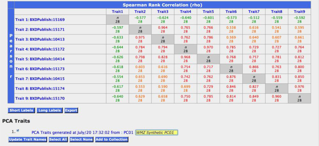
Correlation matrix of nine water maze (WMZ) traits from Milhaud and colleagues (2002). Traits covary well, and it is therefore useful to statistically represent some of these traits by a principal component (see bottom of figure). In this case a synthetic PC trait can explain over 75% of the total phenotypic variance among genotypes of mice. Synthetic traits can be used like all other standard traits for mapping and behavioral analysis.

A common procedure is to study the correlation among traits and perhaps to reduce the complexity of a set of related traits by computing one or more principal components (PC) from a larger number of correlated traits. To do either (compute correlations or PC data) you need to use the Matrix function toward the top of the Trait Collection window. The result is a correlation matrix (Figure 6), along with other statistical results (Scree and factor load plots, although not shown in the figure). Absolute values of the correlations among the nine traits in Table 1 of Milhaud et al. are above 0.5. You can click on any of these correlations to view the underlying scatterplot. The strong covariation among traits justifies the process of producing consensus PC measures of speed and/or persistence of this spatial memory task. But, this process is unbalanced (eight related traits generated from training trials and only one from the probe trial), so the point is to be careful not to blend away unique biological signals in this process. Here we should redo the analysis and exclude the probe memory trial (trait 15169) and possibly just use the four logged data sets. The result is a synthetic PC-derived trait that combines data for the four test learning trials.

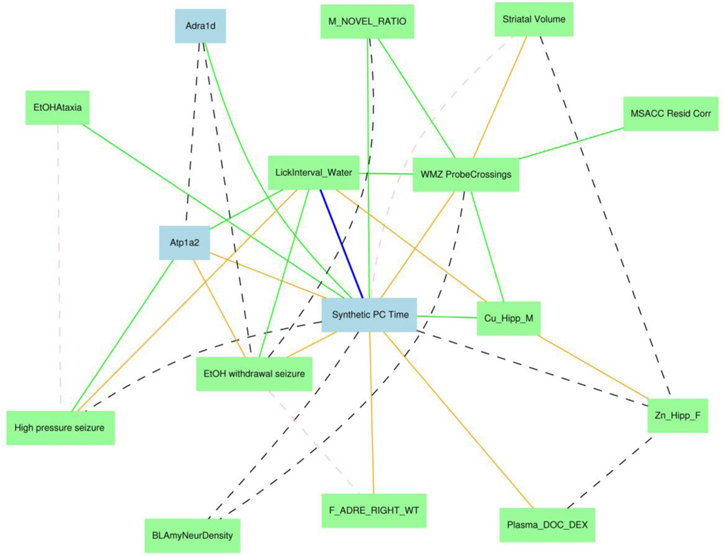
We can now use this synthetic trait to compute correlations to the hundreds of other CNS-relevant traits that have been generated for members of the BXD family (e.g., Phillip et al., 2010). The result of this kind of correlation assembly is a network graph such as that in Figure 7 (see the legend for a list of key steps to make these graphs). Each node is a genetically variable phenotype. The PC trait derived from the time it takes to reach the platform is in the middle (blue), whereas the probe trial crossing data (WMZ Probe Crossing) is above and to the right (green). Links between nodes represent correlations (blue, green, and black dashed = negative correlations, orange and pink dashed = positive correlations). In the original web version of this figure all of the links and nodes are hot and clicking on them either gets to a scatterplot or the set of data. We have already mentioned the correlation between "Lick Interval" and the time to reach the platform—both are probably being driven by a central pattern generator controlled by Atp1a2—and you can see this link explicitly. The Atp1a2 node (blue) represents variation in whole brain expression in the same BXD strains. The node for Adra1d (upper left) represents variable expression of this adrenergic receptor in hippocampus. The other phenotypes in this graph include neuroanatomical traits (e.g., Striatal Volume, MSACC = mid-sagittal area of the corpus callosum), key metabolites and metals (plasma deoxycorticosterone levels, copper levels and zinc levels in hippocampus), and responses to ethanol (ethanol/EtOH ataxia and EtOH withdrawal seizures) and high atmospheric pressure (High pressure seizure). The challenge now is to (1) determine how much of this network is reliable and biologically meaningful; and to (2) understand the molecular, cellular, and environmental processes and mechanisms that produce these patterns of correlation—the collective “black box” located between genes and behavior. Each of the nodes in this network graph can also be studied using the genetic methods that we applied to the water maze data sets, with the hope of uncovering other common candidates that genetically and mechanistically bind apparently disparate traits such as lick rate and the time it takes to swim to a target platform.

Figure 7.

Covariance network of phenotypes related to water maze (WMZ) Probe Crossings. This graph was generated in GeneNetwork by computing Pearson product moment correlations among all members of a set of highly variable anatomical, behavioral, neurochemical, and gene expression data collected for the same types of mice. As long as these traits are collected from the same Group in GeneNetwork—in this case, BXD—they can be added to a Trait Collection. The type of graph shown here is generated by selecting traits from the Trait Collection and then using the Graph option.

Now that you are familiar with network construction and the types of biological questions that can be addressed, we provide a detailed example of a complete network analysis. We examine the impact of a strong mutation in a key enzyme on brain network function. For a more detailed overview of GeneNetwork please see Chesler et al., 2003 and 2005. For detailed network analyses using this web resource please see Li and Mulligan et al., 2010—an example of traits linked to expression of the Comt gene—and Mulligan et al., 2012—an example of the genetic regulation of GABA type-A receptors.

Step 3: Dissecting the Behavioral Impact of Sequence Variants using GeneNetwork

Degradation of key neurotransmitters—including dopamine and norepinephrine—is mediated in part by the enzyme catechol-O-methyltransferase (Comt). A mutation in the 3’ UTR of the strain with the B haplotype leads to the production of a short 3’ UTR and high protein levels compared to strains without the mutation, including the all strains that inherit the D haplotype (Li and Mulligan et al., 2010). Because the Comt gene is polymorphic between the B- and D-type strains, the mutation is segregating in the BXD family. This means that we can use the accumulated wealth of gene expression data, genotypes, and CNS-related phenotypes to explore the impact of this mutation on global brain network function. A remarkable feature is that we can do this without generating any new data—we can strategically and genetically mine data that go back 40 years. In this case we ask the following questions: (1) “Which genes/transcripts map to the genetic mutation in Comt?” and (2) “Which behavioral and neurochemical phenotypes map to the genetic mutation in Comt?”.

We can answer these questions using data and tools in GeneNetwork along with a little background information. The Comt gene is located on Chr 16 at approximately 18.4 Mb. We can use options on the Select and Search page to identify a good marker for that region of the genome. The marker (usually a SNP) allows us to identify those mRNA expression traits and phenotypes that have higher or lower expression associated with the inheritance of that section of DNA from one of the parental types. In this case the analysis is especially straightforward because there are only a few variants located near the Comt gene and Comt is the only candidate within a 2 Mb genomic interval.

From the home page change Type to Genotypes. Enter the following text into the Get Any box: POSITION=(chr16 17 19). This search will find all markers that are located on Chr 16 between 17 and 19 Mb. For this example we select marker rs4165069. Once you have clicked on the link for this marker you will be directed to the Trait Data and Analysis page where you have many options to explore in great detail the data type you have selected, in this case, our Comt gene marker. Expand the section for Calculate Correlations. Here you can retrieve correlations between the marker and any other data set generated using the BXD family. For Database, select BXD Published Phenotypes. You can choose the number of top correlations to return as well as the type of correlation computed—Pearson or Spearman rank correlation, the latter being less sensitive to outliers. For this example we will use the Pearson correlation. The top correlation between the marker and each BXD phenotype is returned as in Figure 8.

Figure 8.

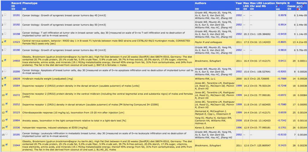
Top correlations between Comt marker rs4165069 and BXD strain phenotypes in GeneNetwork. Highlighted traits are suitable for mapping studies as they have a sufficiently large sample size—generally at least 12, but more is always better.

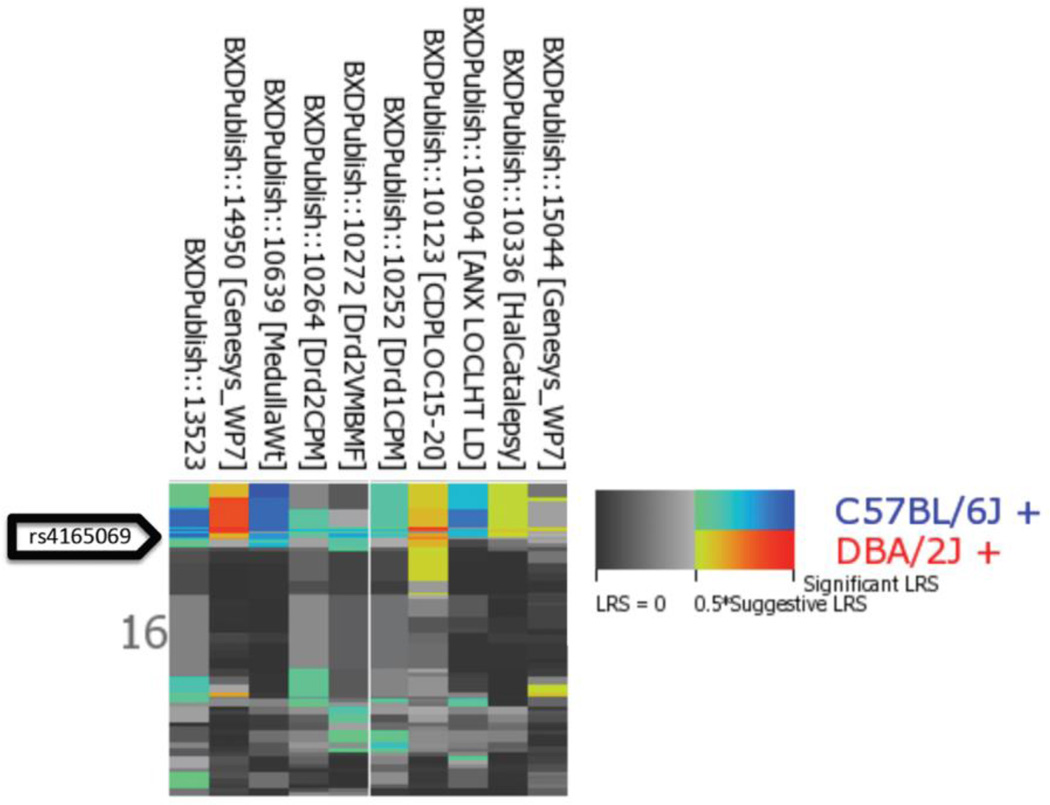
We know from previous sections that the LRS or LOD value is a description of the strength of the linkage between inheritance of parental alleles at a specific genomic region and expression of a trait. As expected, very high marker correlations often have a maximum LRS value near the position of the marker (the location of the Comt gene, shown in the table as Max LRS Location Chr and Mb). As values decrease, we will eventually reach a threshold that is no longer significant. To visualize the mapping of the phenotypes to the location of the Comt mutation select the top 10 phenotypes. (Note: see Figure 8; do not include traits that have N cases less than 12 because small sample size can lead to spurious mapping results or cannot be mapped at all (N < 9)). Next, select the Heat Map option to visualize the mapping of these traits. The results are shown in Figure 9. The top 10 correlates of our marker map precisely to Comt with a suggestive or significant LRS value (Figure 9). This set of phenotypes is “downstream” of the mutation in Comt. In other words, fluctuating levels of Comt mRNA and protein due to the 3’ UTR mutation cause variation in the expression of these phenotypes.

Figure 9.

Multiple trait mapping in GeneNetwork. The Heat Map feature allows for a quick comparison of the genetic regulation of many traits. The Heat Map plots the LRS or LOD values for each allele as a color (blue for the B-type parent and red for the D-type parent) with increasing intensity indicating a stronger associations and lower p values. These values are displayed for each selected trait (X-axis) by chromosomal position (Y axis).

We have illustrated how to locate downstream phenotypes of a gene variant using marker analysis in GeneNetwork, but there is an even more direct way to answer the same question. It is possible to query data sets in GeneNetwork from the Select and Search page using advanced options to locate the highest trait LRS values for any genomic interval, in this case the region within 2 Mb of Comt. (Note: You can explore this and other search options further by clicking the Advanced Search button and reading the section Advanced Searching and General Advice.) From the home page change Type to Hippocampus mRNA and Data Set to Hippocampus Consortium M430v2 (Jun06) RMA. Enter the following text into the Combined search box: MEAN=(8 16) LRS=(9.6 999 Chr16 16 19) transLRS=(9.6 999 5). Using a simple query we retrieve all the genes/transcripts from this particular hippocampal data set that have a mean expression between 8 and 16 [(MEAN=(8 16)] with a maximum LRS value between 9.6 and 999 [transLRS=(9.6 999 5)] located near the mutation in Comt [LRS=(9.6 999 Chr16 16 19)]. This set of hippocampal genes/transcripts—including Apba1, Cmip, and Stau1—is “downstream” of the mutation in Comt.

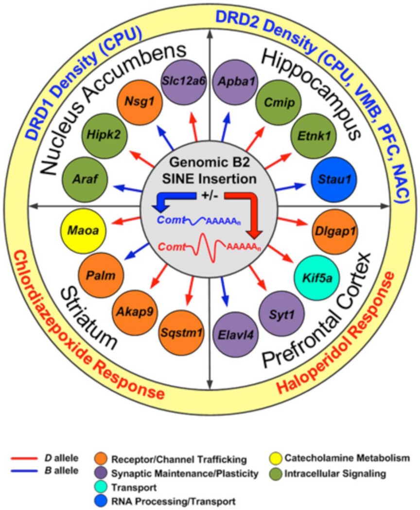
Using advanced search options in GeneNetwork it is possible to quickly mine many different types of data to create gene sets and networks to address specific biological questions. We can combine all of these results (both the behavioral and neurochemical phenotypes and the mRNA microtraits) as shown in Figure 10. This set represents a key part of the Comt functional brain network. While we do not know the biological mechanisms or the number of intervening molecular processes between cause and effect we have established an almost unequivocal causal link between Comt expression level, other mRNA expression levels, and higher order phenotypes. We can now use this highly relevant biological network of causal relationships to address the biological role of Comt in brain and to generate new hypotheses. As might be expected, given its role in the degradation of catecholamine neurotransmitters, alteration in the level of the COMT enzyme has an effect on GABAergic and dopaminergic neurotransmitter systems. Binding affinity of dopamine receptors DRD1 and DRD2 (a measure of receptor density), haloperidol (a dopamine receptor antagonist) response and chlordiazepoxide (an allosteric modulator of GABA type A receptors) response map to the location of the Comt mutation on Chr 16. The expression of genes involved in addiction (Mao, Ptprd, and Slit3) and psychiatric illness (Maoa, Myt1l, Slc12a6, and Slit3) are also controlled by variation in Comt expression. Human mutations in the COMT gene have been associated with schizophrenia, anorexia nervosa, bipolar disorder, anxiety, and substance abuse (Hosak, 2007). Our functional brain network identifies new gene targets and neurotransmitter systems that evidently interact with Comt in similar biological processes and may influence susceptibility to these complex human disorders.

Figure 10.

Comt brain network. The mutation in Comt, actually the insertion of a B2 SINE element in the 3’ UTR of C57BL/6J (Blue Comt gene in figure center), causes the production of a shorter mRNA in the B-Type parental strain. GeneNetwork tools and the wealth of data compiled for the BXD family were used to determine what transcripts and phenotypes mapped back to the physical location of the mutation in the Comt gene. Downstream gene targets of the mutation in Comt are shown in the inner ring and downstream phenotypes are shown in the outer ring for four brain regions. Higher expression of the trait associated with inheritance of the B- or D-type allele is shown in red or blue, respectively. Biological process is indicated by color.

Summary

Having completed this chapter you should now be able to use the resources available on GeneNetwork to explore variation in single genes and behavioral and other phenotypes. We also hope that you have gained expertise in assembling multilevel causal networks and in generating your own synthetic traits to address and test biological questions and hypotheses. We realize that there is still a fairly steep learning curve on some of the work we have reviewed, but the good news is that the resources and on-line tools are getting progressively faster and more streamlined. The on-line documentation (see all of the Help and Reference files on GeneNetwork) will also reduce the energy barrier of adopting powerful systems genetics and systems behavioral approaches. Web services such as GeneNetwork and its companions—GeneWeaver (Baker et al., 2012), WebGestalt (Zhang et al., 2005), DAVID (Huang et al., 2009a; Huang et al., 2009b), and the Allen Brain Atlas (Lein et al., 2007)—can now be used as virtual and free laboratories to test specific biological hypothesis, or they can be used to generate new ideas ab initio.

References

- Baker EJ, Jay JJ, Bubier JA, Langston MA, Chesler EJ. GeneWeaver: a web-based system for integrative functional genomics. Nucleic Acids Res. 2012 Jan;40(Database issue):D1067–D1076. doi: 10.1093/nar/gkr968. 2012. [DOI] [PMC free article] [PubMed] [Google Scholar]
- Boughter JD, Jr, Mulligan MK, St John SJ, Tokita K, Lu L, Heck DH, Williams RW. Genetic control of a central pattern generator: Rhythmic oromotor movement in mice is controlled by a major locus nearAtp1a2. PLoS One. 2012;7(5):e38169. doi: 10.1371/journal.pone.0038169. [DOI] [PMC free article] [PubMed] [Google Scholar]
- Bowler PJ. The Eclipse of Darwinism: Anti-Darwinian Theories in the Decades Around 1900. Johns Hopkins Press; 1983. [Google Scholar]
- Chesler EJ, Lu L, Wang J, Williams RW, Manly KF. WebQTL: rapid exploratory analysis of gene expression and genetic networks for brain and behavior. Nature Neuroscience. 2004;7:485–486. doi: 10.1038/nn0504-485. [DOI] [PubMed] [Google Scholar]
- Chesler EJ, Lu L, Shou S, Qu Y, Gu J, Wang J, Hsu HC, Mountz JD, Baldwin N, Langston MA, Threadgill DW, Manly KF, Williams RW. Genetic dissection of gene expression reveals polygenic and pleiotropic networks modulating brain structure and function. Nature Genetics. 2005;37:233–242. doi: 10.1038/ng1518. [DOI] [PubMed] [Google Scholar]
- Hosak L. Role of the COMT gene Val158Met polymorphism in mental disorders: a review. Eur Psychiatry. 2007;22:276–281. doi: 10.1016/j.eurpsy.2007.02.002. [DOI] [PubMed] [Google Scholar]
- Huang DW, Sherman BT, Lempicki RA. Systematic and integrative analysis of large gene lists using DAVID Bioinformatics Resources. Nature Protoc. 2009;4(1):44–57. doi: 10.1038/nprot.2008.211. [DOI] [PubMed] [Google Scholar]
- Huang DW, Sherman BT, Lempicki RA. Bioinformatics enrichment tools: paths toward the comprehensive functional analysis of large gene lists. Nucleic Acids Res. 2009;37(1):1–13. doi: 10.1093/nar/gkn923. [DOI] [PMC free article] [PubMed] [Google Scholar]
- Kempermann G, Gage FH. Genetic determinants of adult hippocampal neurogenesis correlate with acquisition, but not probe trial performance, in the water maze task. Eur J Neurosci. 2002;16:129–136. doi: 10.1046/j.1460-9568.2002.02042.x. [DOI] [PubMed] [Google Scholar]
- Kempermann G, Chesler EJ, Lu L, Williams RW, Gage FH. Natural variation and genetic covariance in adult hippocampal neurogenesis. Proc Natl Acad Sci USA. 2006;103:780–785. doi: 10.1073/pnas.0510291103. [DOI] [PMC free article] [PubMed] [Google Scholar]
- Krebs J, Römer B, Overall RW, Fabel K, Babu H, Brandt MD, Williams RW, Jessberger S, Kempermann G. Adult hippocampal neurogenesis and plasticity in the infrapyramidal bundle of the mossy fiber projection: II. Genetic covariation and identification ofNos1as a linking candidate gene. Front Neurosci. 2011;5:106. doi: 10.3389/fnins.2011.00106. [DOI] [PMC free article] [PubMed] [Google Scholar]
- Laughlin RE, Grant TL, Williams RW, Jentsch JD. Genetic dissection of behavioral flexibility: reversal learning in mice. Biol Psychiatry. 2011;69:1109–1116. doi: 10.1016/j.biopsych.2011.01.014. [DOI] [PMC free article] [PubMed] [Google Scholar]
- Lein ES, Hawrylycz MJ, Ao N, Ayres M, et al. Genome-wide atlas of gene expression in the adult mouse brain. Nature. Jan 11;445(7124):168–176. doi: 10.1038/nature05453. (200) Epub 2006 Dec 6. [DOI] [PubMed] [Google Scholar]
- Li R, Tsaih SW, Shockley K, Stylianou IM, Wergedal J, Paigen B, Churchill GA. Structural model analysis of multiple quantitative traits. PLoS Genet. 2006;2(7):e114. doi: 10.1371/journal.pgen.0020114. [DOI] [PMC free article] [PubMed] [Google Scholar]
- Li D, Mulligan MK, Wang X, Miles MF, Lu L, Williams RW. A transposon in Comt generates mRNA variants and causes widespread expression and behavioral differences among mice. PLoS One 17. 2010;5(8):e12181. doi: 10.1371/journal.pone.0012181. [DOI] [PMC free article] [PubMed] [Google Scholar]
- Milhaud JM, Halley H, Lassalle JM. Two QTLs located on chromosomes 1 and 5 modulate different aspects of the performance of mice of the BXD Ty RI strain series in the Morris navigation task. Behav Genet. 2002;32:69–78. doi: 10.1023/a:1014412029774. [DOI] [PubMed] [Google Scholar]
- Mozhui RT, Ciobanu DC, Schikorski T, Wang XS, Lu L, Williams RW. Dissection of a QTL hotspot on mouse distal chromosome 1 that modulates neurobehavioral phenotypes and gene expression. PLoS Genetics. 2008;4:e1000260. doi: 10.1371/journal.pgen.1000260. [DOI] [PMC free article] [PubMed] [Google Scholar]
- Mulligan MK, Wang X, Adler AL, Mozhui K, Lu L, Williams RW. Complex control of GABA(A) receptor subunit mRNA expression: variation, covariation, and genetic regulation. PLoS One. 2012;7(4):e34586. doi: 10.1371/journal.pone.0034586. [DOI] [PMC free article] [PubMed] [Google Scholar]
- Onimaru H, Ikeda K, Kawakami K. Defective interaction between dual oscillators for respiratory rhythm generation in Na+,K+-ATPase {alpha}2 subunit-deficient mice. J Physiol. 2007;584:271–284. doi: 10.1113/jphysiol.2007.136572. [DOI] [PMC free article] [PubMed] [Google Scholar]
- Overall RW, Kempermann G, Peirce J, Lu L, Goldowitz D, Gage FH, Goodwin S, Smit AB, Airey DC, Rosen GD, Schalkwyk LC, Sutter TR, Nowakowski RS, Whatley S, Williams RW. Genetics of the hippocampal transcriptome in mouse: a systematic survey and online neurogenomics resource. Front Neurosci. 2009;3:55. doi: 10.3389/neuro.15.003.2009. [DOI] [PMC free article] [PubMed] [Google Scholar]
- Peirce JL, Chesler EJ, Williams RW, Lu L. Genetic architecture of the mouse hippocampus: identification of gene loci with selective regional effects. Genes Brain Behav. 2003;2:238–252. doi: 10.1034/j.1601-183x.2003.00030.x. [DOI] [PubMed] [Google Scholar]
- Philip VM, Duvvuru S, Gomero B, Ansah TA, Blaha CD, Cook MN, Hamre KM, Laviviere WR, Matthews DB, Mittleman G, Goldowitz D, Chesler EJ. High-throughput behavioral phenotyping in the expanded panel of BXD recombinant inbred strains. Genes, Brain and Behavior. 2010;8:129–159. doi: 10.1111/j.1601-183X.2009.00540.x. PMID 19958391. [DOI] [PMC free article] [PubMed] [Google Scholar]
- Rietman ML, Sommeijer JP Neuro-Bsik Mouse Phenomics Consortium. Levelt CN, Heimel JA. Candidate genes in ocular dominance plasticity. Front Neurosci. 2012;6:11. doi: 10.3389/fnins.2012.00011. [DOI] [PMC free article] [PubMed] [Google Scholar]
- Shifman S, Bell JT, Copley RR, Taylor MS, Williams RW, Mott R, Flint J. A high-resolution single nucleotide polymorphism genetic map of the mouse genome. PLoS Biol. 2006;4(12):e395. doi: 10.1371/journal.pbio.0040395. [DOI] [PMC free article] [PubMed] [Google Scholar]
- Shipley B. A User's Guide to Path Analysis, Structural Equations and Causal Inference. Cambridge Univ Press; 2002. Cause and Correlation in Biology. [Google Scholar]
- Zhang B, Kirov S, Snoddy J. WebGestalt: an integrated system for exploring gene sets in various biological contexts. Nucleic Acids Res. 2005 Jul 1;33(Web Server issue):W741–W748. doi: 10.1093/nar/gki475. 2005. [DOI] [PMC free article] [PubMed] [Google Scholar]