Interpretational Confounding or Confounded Interpretations of Causal Indicators?

Abstract

In measurement theory causal indicators are controversial and little-understood. Methodological disagreement concerning causal indicators has centered on the question of whether causal indicators are inherently sensitive to interpretational confounding, which occurs when the empirical meaning of a latent construct departs from the meaning intended by a researcher. This article questions the validity of evidence used to claim that causal indicators are inherently susceptible to interpretational confounding. Further, a simulation study demonstrates that causal indicator coefficients are stable across correctly-specified models. Determining the suitability of causal indicators has implications for the way we conceptualize measurement and build and evaluate measurement models.

Many concepts in the social and behavioral sciences are difficult to directly measure. As a result, issues of measurement play a central role in social science research. Measurement can be defined as “the process by which a concept is linked to one or more latent variables, and these are linked to observed variables” (Bollen, 1989, p. 180). In this process, a theoretical concept of interest is first identified. Next, one or more latent variables corresponding to this concept are developed. Latent variables are then linked to observed variables, guided by substantive theory and empirical tests of fit. Researchers commonly use multiple measures to capture each latent variable that represents a concept or dimension of a concept. Importantly, concepts are ideas created by researchers. Further, latent variables represent concepts we wish to measure, ideally with a high degree of correspondence, but the two entities are distinct.

The traditional and dominant approach to measurement is to represent these multiple indicators as dependent on the latent variables they represent. “Effect” or “reflective” indicators¹ are terms that describe indicators that are effects of their latent variable. Nearly all of the measurement theory in the social and behavioral sciences since Spearman’s (1904) factor analytic models have assumed all indicators are effect indicators. This is entirely appropriate for many indicators that can be thought of as arising from a latent variable, but this does not make sense for all indicators.

The general definition of measurement cited above includes effect indicators but does not assume effect indicators. In contrast, other common definitions of measurement do assume effect indicators. For example, in their treatise on construct validity, Borsboom, Mellenbergh, and Heerden (2004) state that “a test is valid for measuring an attribute if and only if (a) the attribute exists and (b) variations in the attribute causally produce variations in the outcomes of the measurement procedure” (p. 1061).

A less traditional specification allows for one or more indicators to function as determinants of the latent variable with an error term that includes the omitted sources of variance in the latent variable. These nontraditional indicators, which are causes rather than effects of the latent variable, we refer to as causal indicators. Misspecification can arise if causal indicators are incorrectly specified as reflective (Jarvis et al., 2003; MacKenzie et al., 2005). However, many researchers specify all indicators as reflective without considering whether effect or causal indicators are most appropriate. Recently, debate has emerged over the utility of causal indicators and their role in measurement. The central issue is whether the coefficients of causal indicators are more sensitive to the outcomes of their latent variable than are effect indicators. More specifically, a widely voiced critique has emerged that the coefficients of causal indicators shift in magnitude depending on the variables that their latent variable predicts and hence the coefficients of causal indicators lack the invariance we would expect for scientific measurement.

In this paper we focus on the issue of whether or not the estimates of causal indicators’ effects on a latent variable are inherently unstable in that they will differ depending on the outcome of the latent variable included in the analysis. Determining the suitability of causal indicators has important implications for how measurement is understood and how measurement models are built and assessed. Notice that the causal indicator specification between observed variables and a latent variable is consistent with the general definition of measurement found in Bollen (1989), but would be excluded from narrower definitions such as that offered by Borsboom et al. (2004). Thus, it is of fundamental importance for the measurement community to understand the meaning of measurement using causal indicators. We hope to address this need through a careful discussion of meanings, terminology, and implications of measurement using causal indicators and effect indicators. To begin, we will review terminology and set up both sides of the debate. We will then examine an empirical example that is the basis for this claim and show that the models in this example are misspecified. We will follow this up with a simulation example where we know the true generating model is correctly specified and can more clearly address the issues under dispute. In anticipation of our results, in this paper we show that the claim of inherently unstable coefficients for causal indicators has little basis in the past literature or in the examples we present here.

Terminology and Models

A large part of the disagreements in this area may be traceable to differences in terminology and meanings of the different types of indicators. Though no one paper can claim to have the “true” terminology and meanings, authors are able to and should define their use of terms. The intention of this section is to define our terminology.

Effect Indicators

Measurement in the factor analytic and item response theory traditions assume effect indicators (also called reflective indicators), which conceptually are dependent on a latent variable. For example, we might define the concept "depressed affect" as "the degree to which a person is experiencing sadness or unhappiness." The concept of depressed affect is represented by a latent variable when we build our measurement model. Responses to a question about the degree to which an individual is feeling sad would form one indicator. Responses to questions on "how blue are you feeling" and "do you consider yourself unhappy" would also be indicators. These questions all correspond to our definition of the concept of depressed affect. As such these indicators share conceptual unity in that they all correspond to the same dimension of the same concept (see Bollen & Bauldry, 2011). But how do the indicators relate to the latent depressed affect variable? Here we can conceive of a mental experiment where an individual's depressed affect is elevated or reduced. We would anticipate that all three indicators would on average simultaneously rise or fall with these changes. The indicators conceptually depend on the latent variable and thus they are effect or reflective indicators.

More generally, a set of effect indicators of a single latent variable should share conceptual unity (i.e., correspond to the definition of the concept) and the latent variable that represents the concept should influence each effect indicator. When the latent variable takes different values, these differences should theoretically be reflected in all the effect indicators simultaneously. Reflective indicators are linear combinations of the latent variable plus an error term:

$$\begin{array}{l}{y}_{1i}={\lambda }_{11}{\eta }_{1i}+{\epsilon }_{1i}\hfill \\ y_{2i}={\lambda }_{21}{\eta }_{1i}+{\epsilon }_{2i}\hfill \\ ⋮\hfill \\ y_{Pi}={\lambda }_{P1}{\eta }_{1i}+{\epsilon }_{Pi}\hfill \end{array}$$ (1)

where y_pi is the pth indicator of η_1i, each λ_p1 is the factor loading describing the expected effect of η_1i on y_pi, and ε_pi is the measurement error for the ith case and pth indicator. In this model it is assumed that y_pi and η_1i are deviation scores² centered at their means, ε_pi and η_1i are uncorrelated, and the E[ε_pi] = 0. Here and throughout the paper the terms effect indicators or reflective indicators refer to the same type of measures, formally defined in equation (1).

Causal Indicators

Causal indicators, like effect indicators, begin with a concept and a theoretical definition of that concept, and we use latent variables to represent each concept in a model. Additionally, causal indicators of the same latent variable should exhibit conceptual unity in that they correspond to the meaning of the same concept. But in contrast to effect indicators, we hypothesize that the indicators influence the latent variable.

The degree of social interaction provides an example (Bollen & Lennox, 1991). Suppose we define the degree of social interaction as the amount of time spent with others. Indicators of time spent with family, with friends, with coworkers, and on social media all indicate the degree of social interaction and hence exhibit conceptual unity. However, theoretically we do not expect the latent variable to drive these indicators simultaneously as expected for the depression indicators. More specifically, if we imagine increasing or decreasing the degree of social interaction of a person, it is more difficult to defend the view that all the indicators will rise or fall in sync with these differences. Alternatively, imagine that the time spent with friends, coworkers, and on social media are held constant, but we increase the time spent with family. The difference in this one indicator would be sufficient to increase the latent variable of social interaction. A similar mental experiment could be run for each indicator and would lead to the same conclusion: these are causal indicators. Similarly, we would expect time spent playing violent video games, watching violent movies, and watching violent television shows to be causal indicators of exposure to media violence.³

Causal indicators are represented in Equation (2). as

$${\eta }_{1i}={\gamma }_{11}{x}_{1i}+{\gamma }_{12}{x}_{2i}+\dots +{\gamma }_{1Q}{x}_{Qi}+{\zeta }_{1i}$$ (2)

where the x_qi are the Q observed causal indicators that affect the latent variable for the ith case: η_1i, each γ_1q describes the expected change in η_1i accompanying a one-unit increase in x_qi holding constant all other xs, and ζ_1i is the latent disturbance which is the collection of all other influences that affect η_1i but are not known or available. For all cases i it is assumed that the E[ζ_1i] = 0 and for all i, j, and q Cov(x_qi, ζ_1j) = 0 (for more on model assumptions in SEM, see Bollen,1989). Additionally, a model with causal indicators is not identified without two or more effect indicators or outcomes in the model for η₁, as in Equation (1). They need not intercorrelate, but correlations among xs are usually freely estimated (Bollen & Lennox, 1991; MacCallum & Browne, 1993).

This distinction between causal and effect indicators is important theoretically for researchers to more accurately understand the constructs they are measuring, and further this distinction has a considerable impact on model building. Because causal indicators are not necessarily expected to increase simultaneously, they may not be highly correlated and generally would not exhibit good factor structure like effect indicators (Bollen & Lennox, 1991). Specifying causal indicators as effect indicators leads to biased parameter estimates (Jarvis et al., 2003; MacKenzie et al., 2005). Aguirre-Uretta and Marakas (2012) suggested that bias may appear to be less extensive in the standardized coefficients, however as Petter, Rai, and Straub (2012) point out, fit will still suffer and many researchers nevertheless use unstandardized estimates. Whereas a model with several effect indicators is identified on its own, a model with only causal indicators is more difficult to identify and generally requires two or more outcomes or effect indicators (Bollen, 1989; Bollen & Davis, 2009; MacCallum & Browne, 1993). Bollen and Ting (2000) developed an empirical test for distinguishing between causal and effect indicators, and strategies for interpreting and assessing the validity of causal indicators (Bollen, 1989; 2011; Cenfetelli & Bassellier, 2009; Diamantopoulos & Winklhofer, 2001; Fayers & Hand, 2002) have also been explored. As discussed in the next section, we differentiate causal indicators from composite indicators and covariates.

Types of Indicators that can Influence Latent Variables

At this point it is helpful to make an important distinction between causal indicators and other types of variables on which a latent variable depends. This distinction was not clearly laid out until recently (Bollen & Bauldry, 2011), where they distinguish between causal indicators, composite indicators, and covariates (see also Bollen, 2011).

Composite indicators form a composite variable which does not carry a disturbance term and therefore the composite variable is not a latent variable in the sense of being unobserved. That is, if we know the coefficients of the composite indicators, we can completely and exactly determine the value of the composite variable. Composite variables are exact linear combinations of their indicators:

$$C_{1i}=w_{10}+w_{11}{x}_{1i}+w_{12}{x}_{2i}+\dots +w_{1Q}{x}_{Qi}$$ (3)

where C_1i is a composite variable formed for case i. Composite variables are weighted combinations of individual measures. Both the composite indicators and their weights can be arbitrary or the weights might be determined by empirical procedures such as principal components analysis or partial least squares. Composite indicators need not have the conceptual unity necessary for measures of the same concept. Whereas causal indicators imply invariant effects on the latent variable, composite variables formed with composite indicators can shift depending on the composite’s outcome(s) (Bollen & Bauldry, 2011).

Covariates are the third type of variable that can influence a latent variable; these are control variables and not indicators. Covariates can influence a latent variable without being an indicator for that variable. For example, gender or ethnicity impact many latent variables, but these variables usually do not measure the latent variable. Causal indicators and covariates can influence the same latent variable; the distinction between these two types of variables depends on theory and is made by the researcher. Causal indicators have conceptual unity in that each is a measure of the same unidimensional concept. Covariates might affect the latent variable but are not measures of it.

The use of the term “formative indicators” is ambiguous in most of the methodological literature. Sometimes the term refers to causal indicators as defined above, however often it follows the definition we give for composite indicators. Models with causal indicators may also be thought of as traditional multiple-indicator multiple cause (MIMIC; Jöreskog & Goldberger, 1975) models, although MIMIC models are more general and do not distinguish between covariates and causal indicators. To avoid confusion, we will follow the distinctions made by Bollen and Bauldry (2011) and use the terms causal and composite indicators as we defined above, and we will refrain from the term formative indicators. The only exception is when we quote other researchers who use the term, and in this case we will do our best to interpret how they are using it.

Debate Concerning Measurement and Causal Indicators

Recently the stability of causal indicator coefficients has been an area of methodological debate. Arguing for instability, Howell, Breivik, and Wilcox (2007a) published an article where among many charges leveled against the use of causal indicators, most importantly the authors asserted that latent variables influenced by causal indicators are more prone to interpretational confounding than traditional latent factors with effect indicators (see also Wilcox et al., 2008). Though they used the term “formative”, their equations demonstrate that they referred to both causal and composite indicators as given in our definitions (Equations 2 and 3). Interpretational confounding occurs when the meaning of a construct is different from the meaning intended by the researcher (Burt, 1976). The danger of interpretational confounding, Burt explained, is “Inferences based on the unobserved variable then become ambiguous and need not be consistent across separate models” (p. 4). Generally, we expect measures of the same latent variable to have a stable relation to the latent variable. The coefficients from the measure to the latent variable should not change regardless of the other variables influenced by the latent variable. As interpretational confounding is clearly a serious danger to cumulative science, the claims made by Howell et al. (2007a) merit careful consideration.

Methodologists agree that interpretational confounding is a potential danger for any variable regardless of indicator type (Bollen & Lenox, 1991; Jarvis et al., 2003), but Howell et al. (2007a) have argued that causal indicators are particularly sensitive to this misspecification. The central claim in their 2007 paper is that “Under the formative [causal indicator] model, the nature of the construct must change as its indicators, dependent variables, and their relationships change” (p. 209). Specifically, the authors claimed that the coefficients connecting causal indicators to a latent variable will vary depending on the outcome variables of that same latent variable. Because the causal indicator coefficients will allegedly shift according to the variables influenced by the latent variable, Howell et al. (2007a) recommended the use of causal indicators be abandoned—having stated that it is impossible to accumulate knowledge about theoretical constructs measured by causal indicators (p. 212).

Arguing that causal indicator coefficients are expected to be stable, an alternative explanation has been offered that interpretational confounding is not inherent to causal indicators, but is rather caused by structural misspecifications of models (Bollen, 2007). Bagozzi (2007; 2010) has in general taken a less firm position and allows that causal indicators may be appropriate in some cases. However Bagozzi has agreed with the assumed limitations of causal indicators and asserted that “Not only would statements of generalizability be problematic with formative variables and their measures, but internal consistency for any particular study could vary, depending on what dependent variables were included or excluded” (2007; p. 8). Citing the concerns articulated by Howell et al. (2007a) and others, Edwards (2011) and Treiblmaier, Bentler, and Mair (2011) have proposed complicated strategies to avoid the use of causal indicators.

Other methodologists have noted the contradictory claims made regarding the stability of causal indicators and have advocated for more research to resolve the dispute and communicate unified recommendations to applied researchers for how to appropriately use causal indicators, should they be found robust under certain assumptions. Diamantopoulos, Riefler, and Roth (2008) wrote a review article for researchers “to encourage the appropriate use of formative [causal] indicators in empirical research while at the same time highlighting potentially problematic issues” (p. 1204). Hardin, Chang, Fuller, and Tokzadeh (2011) accepted the cited work as evidence of the limitations of causal indicators and suggested that theory is sorely lacking to guide researchers in the principled use of causal indicators. Finally, Hardin and Marcoulides (2011) called for a moratorium on the use of causal indicators while methodologists reach a consensus on this issue of the suitability of causal indicators and communicate that consensus to applied researchers. Determining whether causal indicators are inherently subject to interpretational confounding should be a priority for measurement researchers since the theoretical distinction between indicator types is nontrivial.

At least two articles have moved the debate from theoretical to empirical and began to evaluate the stability of causal indicator coefficients. Kim, Shin, and Grover (2010) and Wilcox et al. (2008) published empirical examples that they claimed demonstrated that causal indicator coefficients change across models and interpreted this change as evidence of interpretational confounding. In both of these examples the authors constructed models with causal indicators influencing a latent variable which in turn affects two other latent variables as in Figure 1A. In a separate model one or both of these outcome latent variables was exchanged for another as in Figure 1B. Kim et al. (2010) and Wilcox et al. (2008) compared the coefficients of the causal indicators across these two models and concluded that the causal indicators significantly differed and hence demonstrated the inherent instability of the coefficients of causal indicators. Additionally, Hardin et al. (2010) showed some differences in causal indicator coefficients when estimating a model using a subsample versus a full sample; however standard errors and other information needed to determine if this change was meaningful were not included.

Figure 1.

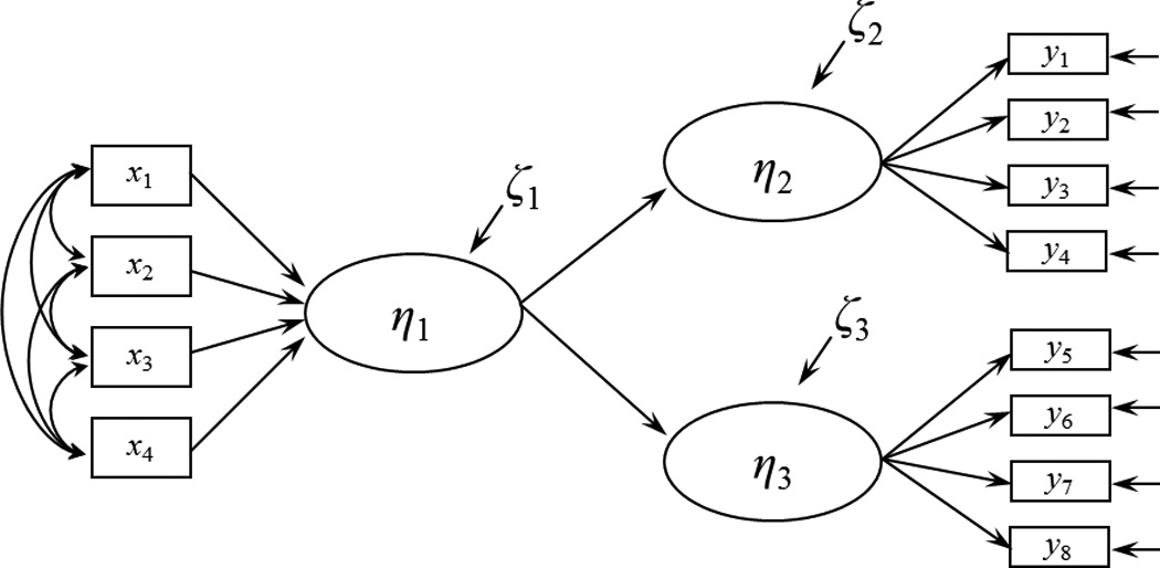
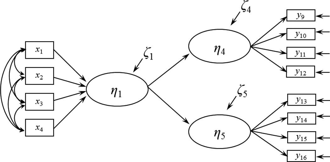
Submodels from simulated example in Wilcox et al. (2008).

On initial examination these results appear to support the claim of coefficient instability of causal indicators. However in both demonstrations the authors did not check some fundamental assumptions that their design implies. Specifically, Kim et al. (2010) and Wilcox et al. (2008) did not test the assumption that the same latent variable (η₁) influenced all outcomes in the model (η₂ – η₅). If this implied full model, as shown in Figure 2, does not fit then the same latent variable does not influence all outcomes, and the construct measured by causal indicators will not be the same across models. That is, structural misspecification may have been the cause of different coefficients in these examples rather than an inherent property of causal indicators. The examples provided by Kim et al. and Wilcox et al. do not report the fit of this full model, and therefore it is unclear whether their results can be attributed to model misspecification (this would be the case if the full models do not fit) or evidence that causal indicators are inherently unstable (this would be the case if the full models are correctly specified).

Figure 2.

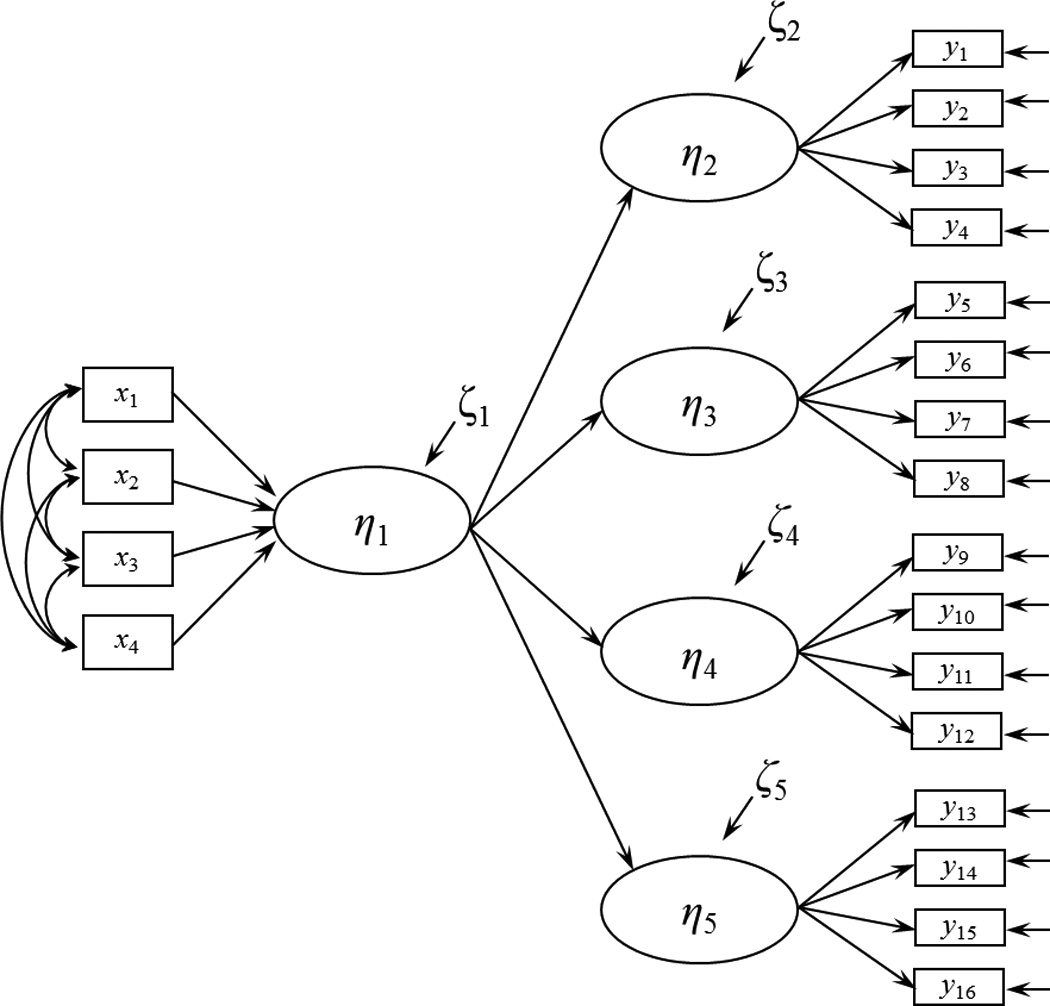
Full model implied by the design of the example in Howell et al. (2008).

These authors also omit an examination of an equivalent assumption that underlies the use of effect indicators; if a set of effect indicators do not measure the same latent variable, the stability of the factor loadings can vary depending on the subset of effect indicators used. This is a basic tenet of factor analysis, and similarly, the coefficients from the latent variable with causal indicators to the outcome latent variables might differ if all outcome latent variables do not depend on the same latent variable. These authors did not assess whether the coefficients from the latent variable defined by causal indicators (η₁) to the outcome latent variables (η₂ – η₅) were stable across the models in Figures 1A and 1B and in a model that includes all outcome latent variables together. Ultimately, these claims of interpretational confounding depend on the full, untested models being correctly specified.

The initial aim of this paper was to test both examples for structural misspecification and for the stability of all coefficients across models with the data used by Kim et al. (2010) and Wilcox et al. (2008). We contacted Kim et al. to obtain the raw data or covariance matrix among all the variables, but the authors declined our request to share the data. Wilcox et al. (2008) included the full covariance matrix corresponding to their example in their paper, so we will proceed to test the full model with these data. We use these data to test the fit of the model that includes all latent variables together and to examine the stability not just of the causal indicator coefficients but also the coefficients relating the source latent variable to the outcome latent variables.

Fitting the Full Model to the Wilcox et al. (2008) Example

We will now examine the example published in Wilcox et al. (2008), which corresponds to Figures 1A and 1B and the estimates for Models 1A and 1B in Table 1. This example consists of simulated data from a population model that is perfectly correct in both sub-models, Model 1A and Model 1B. This is evidenced by the near-zero Chi-square statistics, each equal to 0.031 with 46 degrees of freedom. We fit the two sub-models previously published and the full model (Model 2) to the covariance matrix provided by Wilcox et al. (2008) using maximum likelihood estimation in Mplus version 6.11 (Muthén & Muthén, 1998–2010), and all estimates are shown in Table 1. Sample size was not reported in Wilcox et al. (2008). However from their reported chi-square statistics and the discrepancies between the covariance matrix and each model, it appears that they used a sample size of N=500.

Table 1.

Sub-models and Full Model Fit to Data Provided by Wilcox et al. (2008)

		Model 1A η2 η3		Model 1B η4 η5		Model 2 η2 – η5
		Est	SE	Est	SE	Est	SE
Path
	η1 → η2	.696	.051			.404	.050
	η1 → η3	.397	.033			.359	.042
	η1 → η4			.060	.026	.291	.036
	η1 → η5			.100	.043	.224	.030
	x1 → η1	1.000		1.000		1.000
	x2 → η1	.804	.095	2.008	1.014	.857	.160
	x3 → η1	.608	.086	4.025	1.834	.755	.152
	x4 → η1	.407	.078	5.011	2.247	.580	.140
R2 value
	η1	.663	.032	.504	.043	.432	.035
	η2	.971	.031			.625	.032
	η3	.650	.035			undefineda
	η4			.525	.049	.915	.027
	η5			.923	.055	.343	.038
Chi-sq(df), p-value		0.031 (46), p = 1.000		0.031 (46), p = 1.000		825.59 (160), p = 0.000
RMSEA		0.000		0.000		0.091
TLI		1.016		1.022		0.896

Note. Solution for full model is not positive definite. Estimated residual variance for η₃ is −0.020. Sample size was not reported in Howell et al. (2008). From their reported chi-square statistics and the discrepancies between the covariance matrix and each model, we determined that they used a sample size of N=500.

^aR² is undefined for η₃ in the full model because the residual variance for η₃ was not significant

The fit of each sub-model is essentially perfect as indicated by the Chi-square statistics already mentioned, RMSEA (both 0.000), and TLI (1.016 in Model 1A and 1.022 in Model 1B). However, there is ample evidence that the full model is misspecified. The fit of the full model is poor; in fact, the estimates of the model included an improper solution. The latent variable covariance matrix Ψ is not positive definite due to a negative estimate of the residual variance of η₃(=−0.020). The chi-square test of model fit is highly significant with a value of 825.59 on 160 degrees of freedom. If there were no specification error, then we would expect the chi-square to be essentially zero given the population nature of the data. The RMSEA is 0.091 and the TLI is 0.896; both indices indicating marginal to poor model fit. But most convincing is the big difference in the fit of the sub-models compared to the full model.

The shift in causal indicator coefficients from the model with η₂ and η₃ to the model with η₄ and η₅ is indeed dramatic, but these differences are unsurprising given that the full model does not fit. For example, the coefficients from x₂ to η₁ and x₃ to η₁ were .804 (.095) and .608 (.086) in Model 1A and increased to 2.008 (1.014) and 4.025 (1.834) respectively, with standard errors in ( ). This large shift in coefficients was accompanied by an equally large shift in standard errors, reflecting increased uncertainty in the parameter estimates for Model 1B. The R-square for each latent variable also shifted dramatically from the sub-models to the full model (for example the R² value for η₂ decreased from .971 in Model 1A to .625 in Model 2), and this is another indication that the full model is misspecified because the same construct (η₁) does not influence all outcomes (η₂ – η₅). Modification indices suggested widespread misspecification in the model, with high values for a large number and variety of omitted paths. We were unable to reach acceptable model fit or circumvent estimation errors by freeing many of these parameters.

It is also interesting to note that the effect "indicator" coefficients relating η₁ to η₂ – η₅ were not more stable than the causal indicator coefficients, and they also shifted considerably from each of the submodels to the full model. According to Wilcox et al. (2008) effect indicators (or effect latent variables by extension) should exhibit greater stability than causal indicators. Following their logic, we would expect that the coefficients from η₁ to η₂, η₃, η₄, and η₅ should be roughly the same in any model that uses a subset of η₂ to η₅ compared to the model that uses all of them together. This is not what we found. Consider Model 1B. The coefficients for η₁‘s effect on η₄ and η₅ are .060 (.026) and .100 (.043). However, in the full model, the same coefficients are estimated to be .291 (.036) and .224 (.030). There is a significant difference in the coefficients for the reflective latent variables which runs counter to Wilcox et al.’s suggestion.

These results suggest that there is still no concrete empirical evidence that causal indicator coefficients are more unstable than effect indicator coefficients. When the full empirical model from Wilcox et al. (2008) is analyzed we find that causal indicators are no more sensitive than effect indicators in a misspecified model. To establish that the coefficients of causal indicators are more unstable would require finding a model that is correctly specified (i.e. valid) that has both causal and effect indicators and demonstrating that the coefficients of the causal indicators depend upon the subset of effect indicators that are used. In such a model, it also should be demonstrated that the coefficients for the subset of effect indicators that are used are stable while those of the causal indicators are not.

So far we have shown that in an improperly specified model, causal indicator coefficients may change depending on the endogenous constructs included in the model, and likewise effect indicator coefficients are unstable in the exact same sets of models. Our next step is to examine the stability of causal indicator coefficients across sub-models when the full model is correct. In order to know the population generating model, we used a computer simulation study to accomplish this goal.

Sensitivity of Causal Indicators in Properly Specified Models

Howell et al. (2007a, 2007b), Kim et al. (2010), and Wilcox et al. (2008) have contended that interpretational confounding is likely to occur when the variables dependent on a latent variable influenced by causal indicators are varied. Specifically they have argued that the causal indicators’ coefficients to their latent variable are unstable and depend on the variables influenced by the latent variable with causal indicators. In his 2007 reply, Bollen included a small simulation demonstration to refute this claim; however the model was not the same as in Wilcox et al. (2008), only a single sample was used, and no factors were varied. Therefore to directly evaluate these claims, we developed a simple simulation study to assess the stability of causal and effect indicators under a variety of conditions. Because our results in the previous section demonstrate that there is no single true model consistent with the Wilcox et al. (2008) example, we could not use it as the basis of our simulation. Instead, we generated data in order to know the true model structure and varied the parameters to examine the stability of causal indicator coefficients, given that the underlying model is correctly specified. We did however base our simulation off of the basic structure used by Kim et al. (2010) and Wilcox et al. (2008). We performed all data generation and estimation via maximum likelihood using Mplus version 6.11 (Muthén & Muthén, 1998–2010).

Using the model shown in Figure 2 as the population generating structure, we manipulated two factors to examine sensitivity to interpretational confounding: (1) the pattern of factor loadings, and (2) the sample size. Factor loadings were varied across three conditions to reflect a range of estimates that commonly arise in social and behavioral science research: the three conditions were (a) all medium factor loadings of 0.5, (b) all large factor loadings of 0.8, and (c) mixed factor loadings, alternating 0.5 and 0.8. These three factor loading conditions were crossed with small, medium, and large sample sizes, doubling sequentially in size, N=125, N=250, and N=500. As in the Wilcox et al. (2008) example, the first latent variable was scaled by setting a single causal indicator coefficient to 1.0. The correlations between all causal indicators (x₁ – x₄) were set to 0.2 in all models.

After generating 500 replications from the full model for each condition, we fit each of the two sub-models (shown in Figure 1A and 1B) and the full model (shown in Figure 2) to each data set. The averaged results for N=250 are displayed in Tables 2–4. The results were essentially the same for the N=125 and N=500 conditions, so these results are omitted for the sake of brevity. We computed mean relative bias (or percentage bias) across all study conditions. This statistic is generally defined as

$$\text{Rel Bias}=\left(\frac{\widehat{\theta }-\theta }{\theta }\right)\times 100,$$ (4)

where θ̂ is the estimate of the parameter and θ is the corresponding population parameter. The percent bias ranged from −0.780 to 2.320 for causal indicator coefficients and from −0.760 to 0.920 for effect indicator coefficients. Relative bias below 5% is generally considered negligible bias. These ranges of relative bias therefore reveal no systematic bias across models for either effect or causal indicator coefficients, and there is certainly no evidence that causal indicator coefficients are more unstable than effect indicator coefficients. There were no systematic differences for the conditions with medium, large, or mixed factor loadings. In summary, we found no evidence of unstable causal indicator coefficients across properly specified models. This finding should be encouraging, as it means that researchers are free to model indicators as directed by theory.

Table 2.

Sub-models and Full Model Fit to Simulated Data with Medium Loadings (N=250)

		Model 1 η2 η3		Model 2 η4 η5		Full Model
Parameter		M Estimate	Rel Bias	M Estimate	Rel Bias	M Estimate	Rel Bias
η1 → η2	.50	.502	0.420			.501	0.280
η1 → η3	.50	.503	0.640			.502	0.480
η1 → η4	.50			.495	−0.980	.496	−0.760
η1 → η5	.50			.503	0.500	.504	0.720
x1 → η1		1.000		1.000		1.000
x2 → η1	.50	.500	−0.020	.503	0.660	.500	−0.100
x3 → η1	.50	.507	1.360	.512	2.320	.507	1.300
x4 → η1	.50	.500	−0.080	.502	0.440	.499	−0.280
Chi-sq(df), p-value		46.343 (46), p = .458		47.367 (46), p = .417		165.301 (160), p = .371
RMSEA		.012		.014		.012
TLI		1.000		.998		.996

Note. Estimates are the means averaged over 500 independent samples. Rel bias is the mean relative (percentage) bias across replications.

Table 4.

Sub-models and Full Model Fit to Simulated Data with Mixed Loadings (N=250)

		Model 1 η2 η3		Model 2 η4 η5		Full Model
Parameter		M Estimate	Rel Bias	M Estimate	Rel Bias	M Estimate	Rel Bias
η1 → η2	.80	.804	0.512			.803	0.350
η1 → η3	.50	.505	0.920			.504	0.700
η1 → η4	.80			.797	−0.350	.799	−0.125
η1 → η5	.50			.503	0.620	.504	0.700
x1 → η1		1.000		1.000		1.000
x2 → η1	.50	.497	−0.620	.501	0.260	.498	−0.380
x3 → η1	.80	.803	0.400	.808	0.950	.804	0.450
x4 → η1	.50	.496	−0.781	.500	−0.060	.497	−0.640
Chi-sq(df), p-value		46.207 (46), p = .464		47.443 (46), p = .414		165.397 (160), p = .369
RMSEA		.012		.014		.012
TLI		1.000		.999		.998

Note. Estimates are the means averaged over 500 independent samples. Rel bias is the mean relative bias across replications.

Conclusions

As noted earlier, Howell et al. (2007a) and Wilcox et al. (2008) do not distinguish between causal and composite indicators in their article. Bollen and Bauldry (2011, p. 7) suggested that though the Howell et al. (2007a) and Wilcox et al. (2008) critiques of causal indicators are unfounded, their criticisms are more applicable to composite indicators. Composite indicators do not have the common conceptual unity shared by causal indicators and the composite to which they contribute is a weighted sum of variables absent an error or disturbance term. In this sense the composite is a somewhat arbitrary combination of variables such that the weights of the indicators can differ with different outcome measures of the composite unless fixed weights are assigned in advance. A composite variable differs from a latent variable, and its meaning can change from model to model. However, a convincing case has not been made that these shortcomings apply to causal indicators.

A near consensus in the literature has emerged that causal indicators’ coefficients are inherently more unstable than are those of effect indicators. The claim does not rest on analytic results, but rather on intuition and an empirical example purported to illustrate the problem. Our paper shows that this intuition is incorrect and that the empirical example marshaled in support of the claim actually is consistent with the idea that structural misspecifications are more responsible for unstable coefficients than are causal indicators. Further, our simulation results indicate that causal indicators should be stable across properly specified models. Model misspecification can occur for a variety of reasons including omitted (or unneeded) paths, variables, dimensions, or correlations among disturbances or exogenous variables. Issues remain regarding estimation, identification, and the meaning of measurement using causal indicators, but contrary to much of the writings in this area, there is no evidence to indicate that the coefficients of causal indicators are inherently more unstable than are those of effect indicators.

Table 3.

Sub-models and Full Model Fit to Simulated Data with Large Loadings (N=250)

		Model 1 η2 η3		Model 2 η4 η5		Full Model
Parameter		M Estimate	Rel Bias	M Estimate	Rel Bias	M Estimate	Rel Bias
η1 → η2	.80	.802	0.287			.802	0.187
η1 → η3	.80	.804	0.550			.803	0.425
η1 → η4	.80			.798	−0.262	.799	−0.113
η1 → η5	.80			.803	0.325	.803	0.412
x1 → η1		1.000		1.000		1.000
x2 → η1	.80	.798	−0.213	.801	0.150	.799	−0.163
x3 → η1	.80	.803	0.350	.807	0.812	.803	0.412
x4 → η1	.80	.797	−0.387	.800	0.000	.798	−0.313
Chi-sq(df), p-value		46.345 (46), p = .458		47.470 (46), p = .413		165.536 (160), p = .366
RMSEA		.012		.014		.012
TLI		1.000		.999		.999

Note. Estimates are the means averaged over 500 independent samples. Rel bias is the mean relative (percentage) bias across replications.

References

- Aguirre-Urreta MI, Marakas G. Revisiting bias due to construct misspecification: Different results from considering coefficients in standardized form. MIS Quarterly. 2012;36(1):123–138. [Google Scholar]
- Bagozzi RP. On the meaning of formative measurement and how it differs from reflective measurement: Comment on Howell, Breivik, and Wilcox (2007) Psychological Methods. 2007;12(2):229–237. doi: 10.1037/1082-989X.12.2.229. [DOI] [PubMed] [Google Scholar]
- Bagozzi RP. Structural equation models are modelling tools with many ambiguities: Comments acknowledging the need for caution and humility in their use. Journal of Consumer Psychology. 2010;20(2):208–214. [Google Scholar]
- Bollen KA. Evaluating effect, composite, and causal indicators in structural equation models. MIS Quarterly. 2011;35(2):359–372. [Google Scholar]
- Bollen KA. Interpretational confounding is due to misspecification, not to type of indicator: Comment on Howell, Breivik, and Wilcox (2007) Psychological Methods. 2007;12(2):219–228. doi: 10.1037/1082-989X.12.2.219. [DOI] [PubMed] [Google Scholar]
- Bollen KA. Structural equations with latent variables. New York: Wiley; 1989. [Google Scholar]
- Bollen KA, Bauldry S. Three Cs in measurement models: Causal indicators, composite indicators, and covariates. Psychological Methods. 2011;16(3):265–284. doi: 10.1037/a0024448. [DOI] [PMC free article] [PubMed] [Google Scholar]
- Bollen KA, Davis WR. Causal indicator models: Identification, estimation, and testing. Structural Equation Modeling. 2009;16(3):523–536. [Google Scholar]
- Bollen K, Lennox R. Conventional wisdom on measurement: A structural equation perspective. Psychological Bulletin. 1991;110(2):305–314. [Google Scholar]
- Bollen KA, Ting KF. A tetrad test for causal indicators. Psychological Methods. 2000;5(1):3–22. doi: 10.1037/1082-989x.5.1.3. [DOI] [PubMed] [Google Scholar]
- Borsboom D, Mellenbergh GJ, Heerden J. The concept of validity. Psychological Review. 2004;111(4):1061–1071. doi: 10.1037/0033-295X.111.4.1061. [DOI] [PubMed] [Google Scholar]
- Burt RS. Interpretational confounding of unobserved variables in structural equation models. Sociological Methods and Research. 1976;5:3–52. [Google Scholar]
- Cenfetelli RT, Bassellier G. Interpretation of Formative Measurement in Information Systems Research. MIS Quarterly. 2009;33(4):689–706. [Google Scholar]
- Diamantopoulos A, Riefler P, Roth KP. Advancing formative measurement models. Journal of Business Research. 2008;61(12):1203–1218. [Google Scholar]
- Diamantopoulos A, Winklhofer HM. Index construction with formative indicators: An alternative to scale development. Journal of Marketing Research. 2001;38(2):269–277. [Google Scholar]
- Edwards JR. The fallacy of formative measurement. Organizational Research Methods. 2011;14(2):370–388. [Google Scholar]
- Fayers PM, Hand DJ. Causal variables, indicator variables and measurement scales; an example from quality of life. Journal of the Royal Statistical Society: Series A. 2002;165(2):233–253. [Google Scholar]
- Hardin AM, Chang JC, Fuller MA, Torkzadeh G. Formative measurement and academic research: In search of measurement theory. Educational and Psychological Measurement. 2011;71(2):281–305. [Google Scholar]
- Hardin A, Marcoulides GA. A commentary on the use of formative measurement. Educational and Psychological Measurement. 2011;71(5):753–764. [Google Scholar]
- Howell RD, Breivik E, Wilcox JB. Is formative measurement really measurement? Reply to Bollen (2007) and Bagozzi (2007) . Psychological Methods. 2007b;12(2):238–245. doi: 10.1037/1082-989X.12.2.205. [DOI] [PubMed] [Google Scholar]
- Howell RD, Breivik E, Wilcox JB. Reconsidering formative measurement. Psychological Methods. 2007a;12(2):205–218. doi: 10.1037/1082-989X.12.2.205. [DOI] [PubMed] [Google Scholar]
- Jarvis CB, MacKenzie SB, Podsakoff P. A critical review of construct indicators and measurement model misspecification in marketing and consumer research. Journal of Consumer Research. 2003;30:199–216. [Google Scholar]
- Jöreskog KG, Goldberger AS. Estimation of a model with multiple indicators and multiple causes of a single latent variable. Journal of the American Statistical Association. 1975;10:631–639. [Google Scholar]
- Kim G, Shin B, Grover V. Investigating two contradictory views of formative measurement in information systems research. MIS Quarterly. 2010;34(2):345–A5. [Google Scholar]
- MacCallum RC, Browne MW. The use of causal indicators in covariance structure models: Some practical issues. Psychological Bulletin. 1993;114(3):533–541. doi: 10.1037/0033-2909.114.3.533. [DOI] [PubMed] [Google Scholar]
- MacKenzie S, Podsakoff P, Jarvis C. The problem of measurement model misspecification in behavioral and organizational research and some recommended solutions. Journal of Applied Psychology. 2005;90:710–730. doi: 10.1037/0021-9010.90.4.710. [DOI] [PubMed] [Google Scholar]
- Muthén LK, Muthén BO. Mplus user’s guide. 6th ed. Los Angeles, CA: Muthén & Muthén; 1998–2010. [Google Scholar]
- Petter S, Rai A, Straub D. The critical importance of construct measurement specification: A response to Aguirre-Urreta and Marakas. MIS Quarterly. 2012;36(1):147–156. [Google Scholar]
- Spearman C. “General Intelligence,” objectively determined and measured. American Journal of Psychology. 1904;15(2):201–292. [Google Scholar]
- Treiblmaier H, Bentler PM, Mair P. Formative constructs implemented via common factors. Structural Equation Modeling: A Multidisciplinary Journal. 2011;18(1):1–17. [Google Scholar]
- Wilcox JB, Howell RD, Breivik E. Questions about formative measurement. Journal of Business Research. 2008;61(12):1219–1228. [Google Scholar]