Profiling small RNA reveals multimodal substructural signals in a Boltzmann ensemble

Abstract

As the biomedical impact of small RNAs grows, so does the need to understand competing structural alternatives for regions of functional interest. Suboptimal structure analysis provides significantly more RNA base pairing information than a single minimum free energy prediction. Yet computational enhancements like Boltzmann sampling have not been fully adopted by experimentalists since identifying meaningful patterns in this data can be challenging. Profiling is a novel approach to mining RNA suboptimal structure data which makes the power of ensemble-based analysis accessible in a stable and reliable way. Balancing abstraction and specificity, profiling identifies significant combinations of base pairs which dominate low-energy RNA secondary structures. By design, critical similarities and differences are highlighted, yielding crucial information for molecular biologists. The code is freely available via http://gtfold.sourceforge.net/profiling.html.

INTRODUCTION

RNA molecules perform a variety of important functions, including the expanding roles of ‘small’ RNAs (1,2). Short, non-coding RNA molecules are now known to function in chemical catalysis as ribozymes (3,4), in aptamer binding as riboswitches (4,5) and in the quorum sensing mechanism of bacteria like Vibrio cholerae (6,7).

Knowing the base pairings of an RNA sequence is critical to understanding its function. A first step is often to predict a minimum free energy (MFE) secondary structure under the nearest neighbor thermodynamic model (NNTM). However, even for short sequences, the MFE prediction may not be the native secondary structure (8,9).

Prediction accuracy improves when suboptimal structures are considered (10–15). Although they can be generated exhaustively (16) or sampled deterministically (17), the current standard is to sample structures stochastically from the Boltzmann distribution (18,19). The goal is to identify the set of base pairs which dominate the low-energy secondary structures and hence are more likely to occur in nature. The challenge is to extract the most meaningful structural signal from a noisy Boltzmann sample.

At the level of individual base pairs, this has been well-studied (20–23). It is known that, even when disjoint, two Boltzmann samples (typically of size 1000) will display ‘nearly identical patterns’ of estimated probabilities (18). Given the significance of high frequency pairings, it is natural to ask which combinations dominate the low-energy secondary structures.

High probability helices, with few low-energy competitors, are a structural signal strong enough to be identified by visual inspection of a 2D dot plot. However, beyond these well-determined regions, the signal is much less clear. In particular, there will be regions where one can easily see that competing structural alternatives exist, but not what they might be.

Clarifying this multimodal signal is critical to advancing our understanding of RNA structure and function. This is especially true for RNAs whose functionality may depend on switching from one conformation to another (4,5). However, identifying combinations of base pairs whose probability is high enough to merit attention but which have significant competing alternatives is challenging.

Existing methods (24,25) identify dominant combinations of base pairs by dividing the Boltzmann sample into groups, and reporting a representative structure for each one. However, as illustrated below, support for different substructures can be lost within a group or diluted across groups. This poses obstacles to understanding the substructural signal in a Boltzmann ensemble, especially when multimodal.

Communicating significant commonalities and differences in pairing combinations is critical to understanding competing structural alternatives for regions of functional interest. Given this, we introduce a new combinatorial approach to analyzing a Boltzmann sample. Our method focuses on denoizing the distribution of helices; those with high enough probability form our set of ‘features’ which are used to ‘profile’ the structures. In this way, we identify notable combinations of helices and present this signal as concisely and stably as possible. By design, RNA profiling highlights critical relations at the substructure level, yielding crucial information for molecular biologists.

VcQrr3: a case study

As concrete motivation, we consider a small RNA sequence with an unknown structure from the pathogen V. cholerae. This bacteria regulates its virulence via a quorum sensing mechanism (26,27) that involves four short, non-coding RNA molecules, denoted VcQrr1–VcQrr4 (6). With cholera infecting three million people and causing 100 000 deaths annually (28), understanding the structure and function of these small RNAs is an important biomedical problem (29).

Quorum regulatory RNA (Qrr) molecules have been found in multiple Vibrio species (6,7,30), and sequence alignment identifies a 32 nucleotide region which is essentially perfectly conserved. This degree of sequence conservation is strong evidence for functional significance; however it provides no structural information for the region of interest.

Moreover, thermodynamic optimization (31,32) predicts that the four VcQrr sequences have three different MFE structures (6) with varying roles for the conserved region. Given this lack of structural consensus, it is important to consider a more nuanced view of base pairing alternatives.

Figure 1 shows the VcQrr3 MFE structure. As seen in Figure 2, base pair probabilities clearly support the formation of the first and fourth helices. However, the situation for the middle two, and most of the conserved region, is considerably murkier; we see that significant structural alternatives exist but not what they might be.

Figure 1.

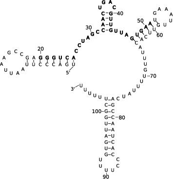
Predicted MFE structure for VcQrr3 with the conserved region (20–51 of 107 nucleotides) shown in bold. VcQrr2 has a comparable four-armed MFE prediction while VcQrr4 has an additional helix forming a ‘cumberbun’ across the middle. VcQrr1 has the common first and last helices, but different base pairings forming a single middle arm.

Figure 2.

Dot plot of base pair probabilities for VcQrr3. Dot size at (x, y) corresponds to log probability of position x pairing with y. Dashed lines indicate the conserved region on each axis. While the first and fourth MFE helices are highly probable, the rest of the sequence—including the majority of the conserved region—has significant suboptimal structural alternatives, as well as many low-frequency pairings.

Parsing this multimodal structural signal requires analyzing the suboptimal structures from a Boltzmann sample. Understanding its nature requires preserving the critical relations. To appreciate the challenge, consider the suboptimal secondary structures for VcQrr3, denoted s₁, s₂ and s₃, shown in Figure 3. As illustrated, they have important commonalities as well as significant differences.

Figure 3.

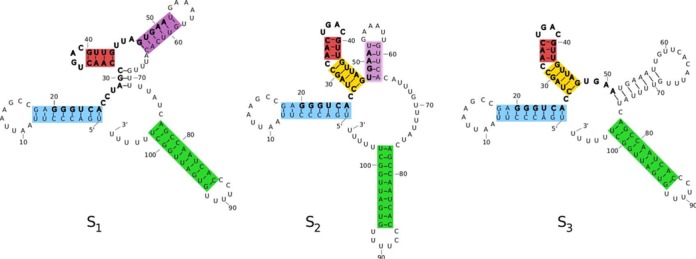
Three structures from a Boltzmann sample for VcQrr3 generated by GTfold (43) with conserved nucleotides 20–51 in bold. Commonalities are highlighted by colored rectangles. Significant differences include pairing 29–31 with 69–71 to form a multiloop in s₁ versus with 43–45 in s₂ and s₃ to form a stem extension (yellow). In s₁ and s₂, 48–50 are paired with 61–63 forming part of a hairpin stem-loop (purple) but are single-stranded in s₃.

The Sfold (18,24,33,34) approach groups structures using divisive clustering under the base pair metric (35), which counts pairings not shared between two structures. The cluster centroid, with minimum distance to all structures in the class, is the representative element. In this way, s₁ and s₂ are clustered together, with the MFE structure from Figure 1 as the centroid, obscuring critical substructural alternatives. Moreover, the similarities with s₃ are not transparent since it belongs to a second (much smaller) cluster.

Alternatively, RNAshapes (25,36,37) groups structures (by default) according to their overall branching configuration. The minimal energy structure with that shape, called a shrep, is the representative element. Both s₂ and s₃ as well as the MFE structure have the four-armed [ ][ ][ ][ ] shape, despite significant differences in the second and third arms. However, the additional ‘cumberbun’ in s₁ gives it the [ ][[ ][ ]][ ] shape, which hides the common base pairs. Moving to a more detailed shape abstraction level helps to distinguish structural differences, but at the cost of significant similarities.

In contrast, profiling focuses on the arrangement of helices at the substructure level. Unlike methods using the base pair metric, we do not distinguish the red and purple helices in s₁ from those containing one less pairing in s₂. However, unlike branching configuration approaches, we do not abstract away all base pair details. Hence, profiling is based on a ‘fuzzy’ definition of helix with a limited degree of elasticity in its exact composition.

We show this degree of abstraction has two benefits. It enables major structural patterns to stand out without getting overwhelmed by minor differences in stem composition. Yet, it retains enough information about specific base pairs to generate experimentally testable hypotheses.

Moreover, our method differs substantially from the existing helix-based analysis approach. Unlike profiling, RNAHeliCes (38,39) does not mine the structural signal from a Boltzmann sample, nor does it classify a given set of secondary structures. Rather, their helix index shape (hishape) abstractions are generated exhaustively starting from the MFE.

These abstractions closely resemble RNAshapes with the refinement that helices are indexed by their ‘central position.’ Thus, the hishape of the VcQrr3 MFE structure is [13, 37.5, 55.5, 89.5] since, for instance, the first arm ends at base pair (8, 18) and . Despite this additional information, hishapes still don't characterize important relations among low-energy secondary structures.

By default, three hishapes for VcQrr3 are output. However, the MFE one still includes s₂. While s₃ is now distinguished (with 63 replacing 55.5), s₁ does not appear unless additional output is requested. However, the number of different hishapes grows exponentially, with much index repetition. But since indices do not correspond uniquely to maximal helices (c.f. Figure 1 of (38)) these are not necessarily similar pairings.

In contrast, profiling identifies well-defined combinations of base pairs that dominate low-energy secondary structures with an emphasis on highlighting significant similarities and differences. This makes it well-suited for probing function, especially for regions with competing structural alternatives.

MATERIALS AND METHODS

Profiling identifies and presents signal on two levels: helices and their combinations. This requires denoizing the set of observed base pairs to highlight the dominant substructures. We employ equivalence classes to consolidate similar substructure elements, and thresholds to highlight the head or core of the distribution. This extracts the signal from our Boltzmann sample, yielding estimated probabilities characteristic of the entire ensemble. By truncating the low-probability tail, we retain the most frequent elements as an informative, concise and reproducible summary of the Boltzmann ensemble.

The profiling pipeline takes a representative sample as input and outputs the substructural signal in the Boltzmann distribution. To begin, we partition the helices in our Boltzmann sample into helix classes. Thresholding yields the most prominent components of helix level signal, which form our set of features. Each structure is categorized according to its combination of features, called a profile. Choosing the highest frequency profiles yields selected profiles, whose relations are visualized in a summary profile graph.

Helix classes

Helices are a fundamental subunit in RNA structures. Under the NNTM, a secondary structure is a set of pseudoknot-free, canonical base pairs. A consecutive run of pairings {(i, j), (i + 1, j − 1), …, (i + k − 1, j − k + 1)} is grouped into a helix denoted (i, j, k). Thus, in Figure 3, s₁ = {(1, 25, 8),(29, 71, 3),(32, 43, 4),(47, 64, 6),(77, 102, 10)}.

When comparing secondary structures, particularly those in a Boltzmann sample, a helix in one may be a proper subset of a helix in another. For instance, the helix (33, 42, 3) in s₂ and in s₃ is a subset of (32, 43, 4) in s₁. At the helix level, this difference is negligible, and all three are colored red in Figure 3. Likewise with the purple helices.

Helix classes are defined to group together helices which are ‘the same’ in this way. More precisely, a helix is maximal if (i − 1, j + 1) and (i + k, j − k) would be non-canonical base pairs or if j − i − 2k < 5. That is, a maximal helix respects the minimum hairpin length of 3 and is non-extendable under the Watson–Crick pairings A ↔ U and C ↔ G as well as the wobble pairing G ↔ U.

A helix class consists of all helices h which are subsets of the same maximal helix g, and will be denoted [g]. Thus, (33, 42, 3) and (32, 43, 4) are elements of the set [(32, 43, 4)], along with four other helices of minimum length ≥2. Given a set of secondary structures S (with multiplicity), profiling identifies the helix classes ordered by descending frequency.

The frequency of a helix h, denoted f(h), is the number of times it appears in S. When S is large enough (typically of size 1000 (18)), then f(h)/|S| is a good approximation to the probability of h in the Boltzmann ensemble and S is called a representative sample. Since (33, 42, 3) occurs in 328 of 1000 sampled structures and (32, 43, 4) in 573, their estimated probabilities are 32.8 and 57.3%.

Similarly, the probability of a helix class c is approximated using its frequency f(c), which is the sum over all f(h) for each helix h in c. Including the frequencies of the other four helices in [(32, 43, 4)], its estimated probability is 94% which is a much stronger signal than any individual helix.

Features

Profiling consolidates similar substructures via helix classes, thereby amplifying their signal. However, there remain many whose signal is weak at best; as illustrated in Figure 4(a), the distribution of frequencies typically has a very long tail. In this case, more than 78% of the VcQrr3 helix classes occur in <1% of the Boltzmann sample.

Figure 4.

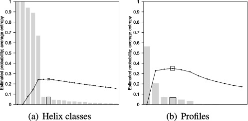
VcQrr3 histograms of estimated probabilities for (a) helix classes and (b) profiles in descending order with graphs of average entropy according to Equation 1 below and its profile equivalent. In (a), the 194 helices observed in the representative sample of 1000 structures were consolidated into 88 helix classes. Only the first 20 are pictured; the estimated probability of the 20th one is 0.8%. In (b), all 13 profiles are pictured but the last seven have frequency <5. The maximum average entropies at the seventh helix class and fourth profile are marked.

Profiling removes the noise of low-probability pairings to highlight significant helices as our features. Hence, helix classes are selected in order of decreasing frequency, up to some threshold. In separating signal from noise, we avoid hard cut-offs, thereby substantially increasing the reproducibility of our results. Instead, profiling identifies the point of diminishing returns, where increasing the number of features begins diluting the structural signal.

This is achieved using the concept of Shannon entropy from the mathematical theory of information. The entropy of a (binary) random variable is a measure of its uncertainty, which is also understood as information gain. The point of diminishing returns in feature selection is determined by the maximum average entropy.

More precisely, the presence of a helix class c in a structure from the Boltzmann sample is a binary random variable X_c. To ensure that the average entropy rises to a maximum, consider the estimated probability normalized by the most probable helix class c₁;

Using this rescaled probability, the entropy of X_c is calculated as

Given observed helix classes c₁, c₂, …, c_m ordered by decreasing frequency, we compute the average entropy at helix class c_k as

(1)

Our threshold t is the index which maximizes this running average, and our set of features is then {c_i∣1 ≤ i ≤ t}.

We can prove that if there exists a k such that , then h_i < h_k for all i ≥ k + 1. Hence, if there is a local maximum h_k, then it is a global one. There are pathological distributions where the average entropy will increase until the last helix class c_m. However, for all observed distributions, the maximum occurs near the beginning of the long tail.

One advantage to thresholding by average entropy is that determining where to truncate the noisy tail is a function of the head of the distribution. Specifically, if the frequencies drop precipitously, this method will retain more low-frequency helix classes than if the decline had been more gradual. In this way, lower frequency alternatives are considered only when they add value to the structural information.

Returning to our VcQrr3 example, we see this behavior illustrated in Figure 4(a), where the maximum average entropy occurs at the 7th helix class—following the steep drop in frequency from the 5th one. (The first eight helix classes are given in Table 1.) Hence, our set of features is {c₁, …, c₇}.

Table 1. Most probable VcQrr3 helix classes c_i and profiles q_i ordered by decreasing observed frequency.

i	Max. helix	f(ci)	Profile	f(qi)
1	(1, 25, 8)	1000	{c1, c2, c3, c4, c5}	564
2	(77, 102, 10)	1000	{c1, c2, c3, c4}	205
3	(32, 43, 4)	940	{c1, c2, c3, c5, c6}	70
4	(47, 64, 7)	891	{c1, c2, c3, c4, c7}	68
5	(27, 47, 5)	669	{c1, c2, c4}	47
6	(51, 75, 7)	74
7	(29, 71, 3)	73
8	(44, 78, 3)	46

The top eight of 88 helix classes and top five of 13 profiles are listed. The maximum average entropy threshold for the helix classes is t = 7, so the set of VcQrr3 features is {c_i∣1 ≤ i ≤ 7}. The threshold for selected profiles is t = 4.

Profiles

Features serve two purposes. First, they highlight the core of the helix class distribution, that is the runs of base pairs which dominate the low-energy secondary structures. Second, they provide the basis for understanding higher order structural signals at the combination-of-helices level.

The profile of a structure s is its maximal set of features. Given the set of features {c₁, …, c₇} from Table 1, the profile of the MFE structure in Figure 1 is {c₁, c₂, c₃, c₄}. This will often be denoted as (1)(3)(4)(2), using parenthetic notation with helix class indices to indicate the nesting relationships. The structures s₁, s₂ and s₃ in Figure 3 have profiles (1)(7(3)(4))(2), (1)(5(3))(4)(2) and (1)(5(3))(6)(2) respectively.

Each profile is an equivalence class of secondary structures. The specific frequency of a profile q, denoted f(q), is the size of this equivalence class, that is the number of structures in the sample S having exactly that set of features. The specific frequencies of the top five VcQrr3 profiles are given in Table 1. Note that the MFE profile is not the most frequent one.

We also define the general frequency of q as the number of structures in S whose profile contains at least those features. Although the specific frequency of the MFE profile q₂ is only 205, its general frequency is 837 since that includes the structures from q₁ and q₄ as well.

Selected profiles

Like helix classes, profiles group together similar structures, thereby amplifying their signal. However, there will also be profiles with a weak signal. As before, we use a maximum average entropy threshold to truncate the distribution yielding our selected profiles.

The denoizing calculations are essentially the same; the association of a profile q to a structure s is a binary random variable X_q. The selected frequency f(q), rescaled by the most frequent profile q₁, yields a probability for the outcomes of X_q which is used to calculate the Shannon entropy. The threshold value t gives the maximum average entropy over the top t profiles, and the set of selected profiles is {q₁, …, q_t}.

Figure 4(b) shows the average entropy against the estimated probability of each VcQrr3 profile. As listed in Table 1, the first, third and fourth selected profiles include (respectively) structures s₂, s₃ and s₁ from Figure 3 while the 2nd includes the MFE.

Selected profiles are maximal probable combinations of helices—a signal from the Boltzmann ensemble above the level of base pair probabilities but below whole structure groupings. As such, they are well-suited for analyzing significant similarities and differences across low-energy secondary structures. This is critical information for a molecular biologist seeking to understand which competing structural alternatives are most likely to occur in nature.

Summary profile graph

As illustrated in Figure 5, the relationships among selected profiles can be visualized graphically. To our knowledge, this is the first such compare/contrast summary of a Boltzmann ensemble, and should be of significant utility to researchers.

Figure 5.

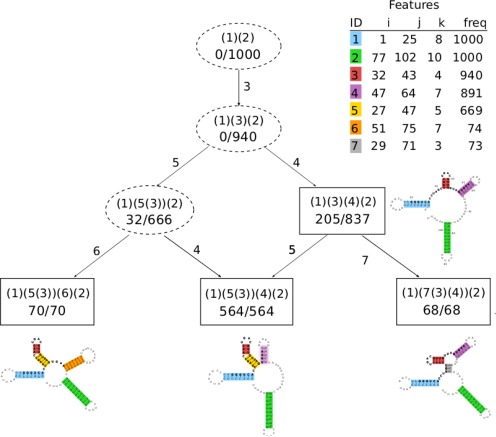
VcQrr3 summary profile graph. Boxes indicate selected profiles, and dashed ovals the intersection ones. Each node is labeled with the profile, in parenthetic notation, along with its specific and general frequencies, written as a ratio. An edge from q to q′ is labeled with the feature(s) from q′∖q. Similarities between profiles are given by the greatest lower bound, aka ‘last common ancestor,’ with differences read from edge labels. The root is always the (possibly empty) profile common to all sampled structures. Features are listed by maximal helix with frequency. For illustrative purposes, the secondary structures from Figures 1 and 3, with features highlighted in color, are shown with their selected profile.

All profiles have a partial order given by set inclusion (q ≤ q′ if q⊆q′) which is visualized as a Hasse diagram. Furthermore, the general frequency of q∩q′ is at least the sum of the specific frequencies for profiles q and q′. Thus while each selected profile is a common combination of features, their intersections are also a significant substructural signal.

To identify common substructures across selected profiles Q = {q₁, …, q_t}, we calculate their intersections I = {q_i∩q_j∣1 ≤ i < j ≤ t}. An intersection profile belongs to I∖Q.

We construct the summary profile graph using the fewest intersection profiles to (weakly) connect all selected profiles. The graph has vertices from I∪Q and directed edges between two profiles if one covers the other in the partial ordering. That is, there is an edge from q to q′ if there is no q″ in I∪Q such that q⊊q″⊊q′.

Since every sampled structure is included in at least one vertex, this graph provides a detailed yet concise overview of the most probable substructures in the Boltzmann ensemble. Reading from the top, the general frequency of the first vertex will always be the size of the Boltzmann sample. Hence, we know that every observed structure includes features c₁ and c₂, and also others since the specific frequency of (1)(2) is 0. Following the first edge, we see that 94% of the sample, and all selected profiles, also include c₃. Beyond this intersection profile, important structural alternatives begin to emerge.

Crucially, these differences all involve base pairs from the conserved region 20–51. For instance, the region 26–31 after c₁ and before c₃ has three distinct possibilities: stem extension (c₅) with 66.6% probability, rare helices or single-stranded with 20.5%, or multibranched loop (c₇) with 6.8%. The first case is read from the intersection profile (1)(5(3))(2) which includes in its general frequency two downstream selected profiles: (1)(5(3))(6)(2) and (1)(5(3))(4)(2). The second and third are the specific frequencies for the other selected profiles which include the MFE structure and s₁, respectively. As will be discussed after the next section, all three cases merit further study and experimentation.

RESULTS

As we have shown, denoizing the VcQrr3 Boltzmann sample yields combinations of base pairs—features and selected profiles—which dominate the low-energy secondary structures. Moreover, as will be discussed next, the value of this substructural signal is maximized by highlighting its multimodal nature, that is the commonalities and differences which provide crucial information for molecular biologists.

First, we give proof-of-principle results that profiling successfully denoises arbitrary Boltzmann samples at this length scale. The 15 test sequences, given in Table 2, all have (i) high sample compression, so that profiling's output is a substantial reduction in scale from the input; (ii) low information loss, so that features and selected profiles cover a disproportionate amount of the observed substructures; (iii) reproducible results, so that variability in threshold cut-offs between independent trials is minimized; and (iv) characteristic frequencies, so that the estimated probabilities extracted from the sample are a true signal from the Boltzmann ensemble. (The last case confirms that denoizing via thresholding introduces no distortions in the substructural signal.)

Table 2. Information for 15 test sequences from five types of short RNA: Qrr, tRNA, 5S ribosomal RNA, THF riboswitch and TPP riboswitch.

Abbr	Seq	Organism (Seq subtype)	Ref	Len	Acc
V1	Qrr	V. cholerae (#1)	(6)	96
V2	Qrr	V. cholerae (#3)	(6)	107
V3	Qrr	Vibrio harveyi (#1)	(7)	95
T1	tRNA	Homo sapiens (Cys)	AC004932	72	0.00
T2	tRNA	Sulfolobu tokodaii (Lys)	BA000023	74	0.45
T3	tRNA	Oryza nivara (Ala)	AP006728	73	1.00
S1	5S	Escherichia coli	V00336	120	0.26
S2	5S	Acheilognathus tabira	AB015591	120	0.59
S3	5S	Desulfurococcu mobilis	X07545	133	0.88
H1	THF	Mitsuokella multacida	ABWK02000009	99	0.11
H2	THF	Clostridium botulinum	CP000939	101	0.43
H3	THF	Streptococcus uberis	AM946015	91	0.62
P1	TPP	Thermoplasma acidophilum	AL445064	107	0.00
P2	TPP	Pasteurella multocida	AE004439	93	0.30
P3	TPP	Bacillus clausii	AP006627	100	0.62

Accession numbers are given for reference when available, and citations otherwise. The tRNA and 5S rRNA sequences and pseudoknot-free secondary structures were obtained from the comparative RNA website (40). The THF and TPP riboswitch sequences and their consensus secondary structures were obtained from the Rfam database (41,42). MFE secondary structures were predicted by GTfold (43) using default settings. The accuracy was calculated as the F-measure, that is the harmonic mean of the MFE sensitivity and positive predictive value against true positive base pairs in the downloaded structures. Sequences were arbitrarily chosen to span the range of MFE accuracies.

For our test set, we selected three Qrr, tRNA, 5S ribosomal RNA, THF riboswitch and TPP riboswitch sequences from online databases (40–42). The average length was 99 nt. In our experience, the strength of the profile signal from a Boltzmann ensemble degrades significantly in the 150–200 nt range. As we will explain further in our concluding remarks, this is consistent with the well-known negative correlation between MFE accuracy and sequence length (8,9), and is the subject of ongoing research.

Although prediction accuracy is typically much higher for short sequences, there is still a wide range overall. Hence, our test sequences were arbitrarily chosen to span the range of MFE accuracies. (The Qrr sequences have unknown native structures and varying MFE predictions.) We observed little correlation with profile characteristics.

For each sequence, we generated 25 Boltzmann samples using GTfold (43). Below and in the Supplementary Data, we report averages and standard deviations across samples for the same sequence, and highlight minimum/median/maximum values for comparisons among the 15 test sequences.

We find that profiling consistently identifies a small set of substructures that dominate the observed base pairing information. These results validate our VcQrr3 case study; by reducing the noise of low-frequency base pairs, profiling extracts a concise and informative substructural signal. Moreover, the thresholding of features and selected profiles is reproducible across multiple runs, and reliably characterizes the Boltzmann ensemble.

High sample compression

A Boltzmann sample typically contains many different helices and secondary structures. Equivalence classes and thresholds reduce the noise of low-frequency base pairs, highlighting the substructural signal presented in features and selected profiles. As seen in Figure 6, and in Supplementary Tables S1 and S2, there are a large number of unique helices on average in each sample and an even larger number of distinct structures.

Figure 6.

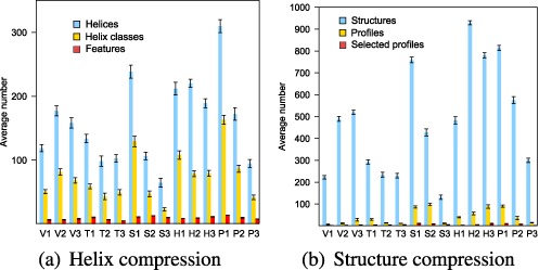
Sample compression via profiling at the (a) helix and (b) combination-of-helices/structure levels. Average number of substructures, respectively helices, helix classes, and features in (a) and structures, profiles, and selected profiles in (b), in 25 samples of 1000 structures for each test sequence. Error bars indicate standard deviations. For additional clarity, a log scale presentation is provided in Supplementary Figure S1.

Consolidating very similar substructures and truncating the low-frequency tails of the distributions produces a much stronger and clearer signal. On average, the number of features and selected profiles are low enough to be investigated by hand—a substantial reduction in scale from the original sample.

We calculated compression ratios for each step and the final results. The typical noise reduction in moving from helices to features is nearly 19-fold and more than 80-fold for structures to selected profiles.

Taken together these numbers demonstrate that profiling consistently extracts a concise core of frequent substructures from a noisy Boltzmann sample.

Low information loss

Importantly, high sample compression does not cost significant structural information. We measure this by calculating the coverage provided by features and by selected profiles, which is the threshold location on the cumulative density function. This is pictured in Figure 7(a) and (b) respectively for VcQrr3, with results for all test sequences in Supplementary Table S3.

Figure 7.

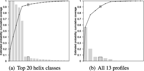
Frequency histograms for VcQrr3 case study with superimposed cumulative distribution functions for (a) the top 20 helix classes and (b) all 13 profiles. Coverage is computed by counting the number of helices (respectively structures) with multiplicity included in the feature set (respectively selected profiles). The features cover 93.8% of observed helices (with multiplicity), and structure coverage for the selected profiles is 90.7%. Results for all test sequences are in Supplementary Table S3.

The information loss in moving from helices to features is very low, since the typical coverage is nearly 90%. The typical selected profile coverage is nearly 83% accounting for a disproportionate amount of the observed structures. Hence, the noise reduction achieved by equivalence classes and thresholds extracts a small set of substructures which dominate the observed base pairing information.

Reproducible results

A significant advantage to denoizing the structural signal from the Boltzmann sample is the reproducibility of profiling across multiple trials. While we certainly cannot remove all variability from this stochastic process, our results confirm a high level of stability in the occurrence of features and of selected profiles.

A feature's stability is the percentage of the 25 trials in which it appears; if a helix class is above the average entropy threshold in 20 Boltzmann samples, its stability is 0.8. We calculate the feature reproducibility of a sample by averaging the stabilities of its features. Each sequence thus has an average feature reproducibility over 25 trials.

As seen in Figure 8(a) and Supplementary Table S4, average feature reproducibility is very high with minimal standard deviation for all test sequences. Hence, there is relatively little variation between sets of features across different trials.

Figure 8.

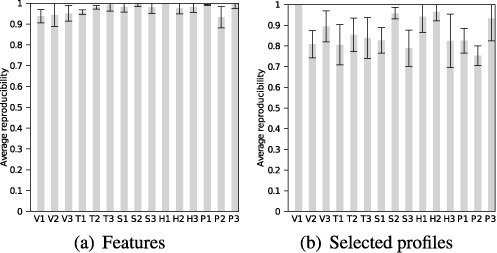
Average reproducibility of (a) features and (b) selected profiles across 25 trials for each of 15 test sequences. Error bars indicate standard deviations.

This analysis is repeated for selected profiles. However, any differences in features will propagate to instabilities in profiles. Hence, as pictured in Figure 8(b), the selected profile reproducibility, while still high, is lower and more variable. Nonetheless, a feature or selected profile output in one trial has a high probability of being output in another.

Characteristic frequencies

Lastly, we confirm that profiling identifies a true substructural signal from the Boltzmann ensemble. Specifically, we measure the reliability of our helix classes and profiles by the standard deviations of their average frequencies across our 25 independent samples. The amount of acceptable variation is benchmarked by the estimated base pair probabilities, a known characteristic signal (18).

For each base pair b, consider the random variable X_b whose values are the different observed frequencies of b across the 25 Boltzmann samples with equal probability. Note that if a base pair does not occur in a sample, its frequency for that trial is zero. The mean and standard deviation of X_b are then μ_b = E[X_b] and .

For VcQrr3, the standard deviations for all 439 observed base pairs are visualized in Figure 9, column (a). Hence, a VcQrr3 structural signal is reliable if the maximum variation in sampled frequencies is on the order of 20 structures.

Figure 9.

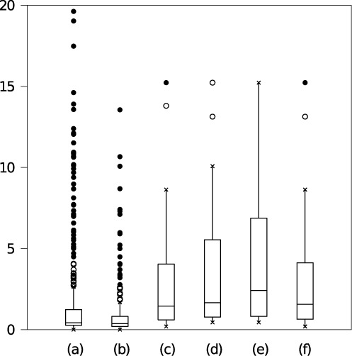
Box plots showing range of standard deviations in frequencies across 25 VcQrr3 Boltzmann samples. Columns correspond to (a) base pairs, (b) helix classes and profiles conditioned on feature sets (c) {c₁ − c₆}, (d) {c₁ − c₇}, (e) {c₁ − c₆, c₈} and (f) {c₁ − c₈}. (Features are indexed in Table 1.) Box midline indicates the median (second quartile). Top and bottom edges mark the first (Q₁) and third (Q₃) quartile, with inter-quartile range R. Whiskers indicate the furthest point within 1.5R of Q₁ and Q₃. Open circles are within 3R; closed circles are beyond.

Repeating this analysis for each of the 236 helix classes observed in 25 trials gives the results in Figure 9, column (b). As expected, consolidating helices into helix classes results in a more reliable signal than individual base pairs.

Yet, there can be small fluctuations in feature selection across different Boltzmann samples. Hence, we confirm that the features from any trial yield characteristic profiles for every trial. Conditioning on a given set of features permits comparisons across all trials, and confirms that the resulting profile frequencies are reliable.

Let F be the set of features for a single Boltzmann sample, and p a profile according to F. We perform the same type of analysis for the random variable X_p across the 25 trials as for the observed base pairs. The results are given in Figure 9, columns (c)–(f) for the four feature sets observed in our 25 VcQrr3 trials. There were 12 profiles with F = {c₁ − c₆}, 15 with {c₁ − c₇}, 18 with {c₁ − c₆, c₈} and 21 with {c₁ − c₈}. (Feature information is in Table 1.) In each case, the standard deviations for profiles are on the order of those for base pairs.

Results for the other test sequences are given in Supplementary Tables S5, S6 and S7 and Figure S2. In all cases, the variability of the profile frequencies for a given set of features is on the order of the base pair frequency variation. Thus, in any given sample, we have confidence that the selected profiles are a true signal from the Boltzmann ensemble.

Hence, a sample of 1000 structures is sufficient for profiling to extract a clear and concise, informative, reproducible and characteristic signal regarding significant combinations of helices for sequences at this length scale.

DISCUSSION

We return to our VcQrr3 motivating example to discuss the benefits of profiling small RNA molecules, especially the generation of experimentally testable hypotheses.

Profiling's balance between abstraction and specificity supports and complements experimental research. By focusing on significant combinations of features, profiling highlights similarities and differences at the substructure level unhampered by sampling noise. With this information, a molecular biologist can target specific nucleotides in experiments to elucidate function.

For example, sequence alignment (6) revealed a highly conserved and likely functional region at nucleotides 20–51 in VcQrr3. According to the summary profile graph in Figure 5, six of the seven features (all but c₂) intersect this region. Both c₁ = [(1, 25, 8)] and c₃ = [(32, 43, 4)] have very high frequency, so the real variation occurs in subregions 26–31 and 44–51.

Nucleotides 26–31 between c₁ and c₃ have three distinct possibilities accounting for 94% of the sampled structures: stem extension for intersection profile (1)(5(3))(2), single-stranded or rare helices for profile p₂ = (1)(3)(4)(2), and multibranch loop for profile p₄ = (1)(7(3)(4))(2). The first is the most probable (66.6%). However, the second (20.5%) includes the MFE structure which closely resembles that for VcQrr2. Furthermore, the third (6.8%) includes the analog of the VcQrr4 MFE structure. Hence, all three cases would merit further study and experimentation.

That a conserved region has a multimodal structural signal is vital information since it suggests possible functional scenarios. For instance, VcQrr3 target activation may require nucleotides 26–31 to be single-stranded. If so, these six nucleotides should have particular functional value.

By now, extensive experiments have tried to pinpoint exact mechanisms for VcQrr target interactions (44,45). This has involved exhaustive, systematic point mutations to verify key functional nucleotides (46–48). Crucially, these experimental results validate the new profiling insights.

Evidence indicates base pairing with four known targets occurs in this subregion: quorum sensing response regulator LuxO at 26–33 (49), high cell density master regulator HapR at 26–45 (7), low cell density master regulator AphA at 5–30 (46,50) and gene vca0939 at 26–44 (44).

Furthermore, certain mutations in the 26–31 subregion knock out function in the last three cases: position 31 for HapR control (47), 25–28 for AphA activation (46) and position 28 for vca0939 (48). Thus, experimental evidence confirms 26–31 as especially important within the conserved region.

The profiling analysis also suggests that subregion 44–51 has a multimodal structural signal. Nucleotides 44–46 are base paired in profiles p₁ and p₃ which contain c₅ and single-stranded or in rare helices in p₂ and p₄. Likewise, 48–50 are base paired in c₄ and not in c₆, which occur in disjoint profiles.

As with 26–31, the different possible structures have functional implications; it may be that base pairing with Qrr targets is regulated by the occurrence of different helix classes. Although this subregion has not yet been the subject of much experimental testing, the single-stranded nucleotides 58–68 in the c₆ hairpin include another region, 58–65, of perfect conservation among Qrr sequences (6).

Thus, profiling identifies two critical subregions within the conserved region revealed by Qrr sequence alignment. Both have multiple different structural possibilities across the selected profiles. The importance of subregion 26–31 is validated by previous experiments, making 48–50 (as well as 58–65) a leading candidate for further investigation. It would be particularly interesting to know if VcQrr3 adopts different profile conformations in vivo, with major biomedical implications if virulence is deactivated in any.

CONCLUSION

For RNA sequences on the order of 100 nt, profiling identifies dominant combinations of base pairs in low-energy secondary structures according to the NNTM. By design, this approach extracts a substructural signal from a Boltzmann sample which is clear and concise, informative, reproducible and reliable. Moreover, by their combinatorial nature, profiles can be easily compared and contrasted, especially through the summary profile graph. Since features are tied to specific base pairs, this computational analysis generates new functional insights, facilitating experimental research such as understanding small RNAs’ role in the mechanisms of cholera.

However, like all thermodynamic RNA secondary structure methods, profiling is fundamentally dependent on the NNTM's approximation of nature. In particular, it is possible to have a strong but inaccurate signal, or to have no strong signal at all, from the Boltzmann ensemble. While this is seldom an issue for short sequences, the problems become more acute as length increases (8,9). These issues manifest in profiling as a combinatorial explosion of profiles for longer sequences, consistent with the exponential growth in the number of possible secondary structures (51) and abstract shapes (25). Thus, although the feature signal remained strong in extensive testing of longer sequences, the profile signal decayed with sequence length.

Nonetheless, profiling has value beyond its demonstrated worth in analyzing small RNAs. It provides a new framework for understanding the scope and limitations of the structural signal from a Boltzmann ensemble, with potential for future enhancements. For example, the distribution of helix classes is an ensemble signature, and its stability under NNTM perturbations can be analyzed, yielding a parametric understanding of this substructure landscape. In summary, the advantages offered by profiling's combinatorial nature and balanced level of abstraction should be of significant utility to both theorists and experimentalists alike.

AVAILABILITY

The RNAStructProfiling C code is freely available via http://gtfold.sourceforge.net/profiling.html.

SUPPLEMENTARY DATA

Supplementary Data are available at NAR Online.

FUNDING

National Institutes of Health [NIGMS R01 GM083621 to C.E.H.]; Burroughs Wellcome Fund [CASI #1005094 to C.E.H.]. Funding for open access charge: Burroughs Wellcome Fund [CASI #1005094 to C.E.H.].

Conflict of interest statement. None declared.

REFERENCES

- 1.Couzin J. Small RNAs make big splash. Science. 2002;298:2296–2297. doi: 10.1126/science.298.5602.2296. [DOI] [PubMed] [Google Scholar]
- 2.Doudna J.A. Structural genomics of RNA. Nat. Struct. Biol. 2000;7:954–956. doi: 10.1038/80729. [DOI] [PubMed] [Google Scholar]
- 3.Breaker R.R. Are engineered proteins getting competition from RNA. Curr. Opin. Biotechnol. 1996;7:442–448. doi: 10.1016/s0958-1669(96)80122-4. [DOI] [PubMed] [Google Scholar]
- 4.Serganov A., Patel D.J. Ribozymes, riboswitches and beyond: regulation of gene expression without proteins. Nat. Rev. Genet. 2007;8:776–790. doi: 10.1038/nrg2172. [DOI] [PMC free article] [PubMed] [Google Scholar]
- 5.Tucker B.J., Breaker R.R. Inventing and improving ribozyme function: rational design versus iterative selection methods. Curr. Opin. Struct. Biol. 2005;15:342–348. [Google Scholar]
- 6.Lenz D.H., Mok K.C., Lilley B.N., Kulkarni R.V., Wingreen N.S., Bassler B.L. The small RNA chaperone Hfq and multiple small RNAs control quorum sensing in Vibrio harveyi and Vibrio cholerae. Cell. 2004;117:69–82. doi: 10.1016/j.cell.2004.06.009. [DOI] [PubMed] [Google Scholar]
- 7.Tu K.C., Bassler B.L. Multiple small RNAs act additively to integrate sensory information and control quorum sensing in Vibrio harveyi. Genes Dev. 2007;21:221–233. doi: 10.1101/gad.1502407. [DOI] [PMC free article] [PubMed] [Google Scholar]
- 8.Mathews D.H., Sabina J., Zuker M., Turner D.H. Expanded sequence dependence of thermodynamic parameters improves prediction of RNA secondary structure. J. Mol. Biol. 1999;288:911–940. doi: 10.1006/jmbi.1999.2700. [DOI] [PubMed] [Google Scholar]
- 9.Doshi K.J., Cannone J.J., Cobaugh C.W., Gutell R.R. Evaluation of the suitability of free-energy minimization using nearest-neighbor energy parameters for RNA secondary structure prediction. BMC Bioinformatics. 2004;5:105. doi: 10.1186/1471-2105-5-105. [DOI] [PMC free article] [PubMed] [Google Scholar]
- 10.Williams A.L., Jr, Tinoco I. Jr. A dynamic programming algorithm for finding alternative RNA secondary structures. Nucleic Acids Res. 1986;14:299–315. doi: 10.1093/nar/14.1.299. [DOI] [PMC free article] [PubMed] [Google Scholar]
- 11.Jaeger J.A., Turner D.H., Zuker M. Improved predictions of secondary structures for RNA. Proc. Natl. Acad. Sci. U.S.A. 1989;86:7706–7710. doi: 10.1073/pnas.86.20.7706. [DOI] [PMC free article] [PubMed] [Google Scholar]
- 12.Zuker M., Jaeger J.A., Turner D.H. A comparison of optimal and suboptimal RNA secondary structures predicted by free energy minimization with structures determined by phylogenetic comparison. Nucleic Acids Res. 1991;19:2707–2714. doi: 10.1093/nar/19.10.2707. [DOI] [PMC free article] [PubMed] [Google Scholar]
- 13.Jacobson A.B., Zuker M. Structural analysis by energy dot plot of a large mRNA. J. Mol. Biol. 1993;233:261–269. doi: 10.1006/jmbi.1993.1504. [DOI] [PubMed] [Google Scholar]
- 14.Zuker M., Jacobson A.B. “Well-determined” regions in RNA secondary structure prediction: analysis of small subunit ribosomal RNA. Nucleic Acids Res. 1995;23:2791–2798. doi: 10.1093/nar/23.14.2791. [DOI] [PMC free article] [PubMed] [Google Scholar]
- 15.Zuker M., Jacobson A. Using reliability information to annotate RNA secondary structures. RNA. 1998;4:669–679. doi: 10.1017/s1355838298980116. [DOI] [PMC free article] [PubMed] [Google Scholar]
- 16.Wuchty S., Fontana W., Hofacker I.L., Schuster P. Complete suboptimal folding of RNA and the stability of secondary structures. Biopolymers. 1999;49:145–165. doi: 10.1002/(SICI)1097-0282(199902)49:2<145::AID-BIP4>3.0.CO;2-G. [DOI] [PubMed] [Google Scholar]
- 17.Zuker M. On finding all suboptimal foldings of an RNA molecule. Science. 1989;244:48–52. doi: 10.1126/science.2468181. [DOI] [PubMed] [Google Scholar]
- 18.Ding Y., Lawrence C.E. A statistical sampling algorithm for RNA secondary structure prediction. Nucleic Acids Res. 2003;31:7280–7301. doi: 10.1093/nar/gkg938. [DOI] [PMC free article] [PubMed] [Google Scholar]
- 19.Mathews D.H. Revolutions in RNA secondary structure prediction. J. Mol. Biol. 2006;359:526–532. doi: 10.1016/j.jmb.2006.01.067. [DOI] [PubMed] [Google Scholar]
- 20.McCaskill J.S. The equilibrium partition function and base pair binding probabilities for RNA secondary structure. Biopolymers. 1990;29:1105–1119. doi: 10.1002/bip.360290621. [DOI] [PubMed] [Google Scholar]
- 21.Hofacker I.L., Fontana W., Stadler P.F., Bonhoeffer L.S., Tacker M., Schuster P. Fast folding and comparison of RNA secondary structures. Monatsh. Chem. 1994;125:167–188. [Google Scholar]
- 22.Huynen M., Gutell R., Konings D. Assessing the reliability of RNA folding using statistical mechanics. J. Mol. Biol. 1997;267:1104–1112. doi: 10.1006/jmbi.1997.0889. [DOI] [PubMed] [Google Scholar]
- 23.Mathews D.H. Using an RNA secondary structure partition function to determine confidence in base pairs predicted by free energy minimization. RNA. 2004;10:1178–1190. doi: 10.1261/rna.7650904. [DOI] [PMC free article] [PubMed] [Google Scholar]
- 24.Ding Y., Chan C.Y., Lawrence C.E. RNA secondary structure prediction by centroids in a Boltzmann weighted ensemble. RNA. 2005;11:1157–1166. doi: 10.1261/rna.2500605. [DOI] [PMC free article] [PubMed] [Google Scholar]
- 25.Giegerich R., Voß B., Rehmsmeier M. Abstract shapes of RNA. Nucleic Acids Res. 2004;32:4843–4851. doi: 10.1093/nar/gkh779. [DOI] [PMC free article] [PubMed] [Google Scholar]
- 26.Miller M.B., Bassler B.L. Quorum sensing in bacteria. Annu. Rev. Microbiol. 2001;55:165–199. doi: 10.1146/annurev.micro.55.1.165. [DOI] [PubMed] [Google Scholar]
- 27.Zhu J., Miller M.B., Vance R.E., Dziejman M., Bassler B.L., Mekalanos J.J. Quorum-sensing regulators control virulence gene expression in Vibrio cholerae. Proc. Natl. Acad. Sci. U.S.A. 2002;99:3129–3134. doi: 10.1073/pnas.052694299. [DOI] [PMC free article] [PubMed] [Google Scholar]
- 28.Mutreja A., Kim D.W., Thomson N.R., Connor T.R., Lee J.H., Kariuki S., Croucher N.J., Choi S.Y., Harris S.R., Lebens M., et al. Evidence for several waves of global transmission in the seventh cholera pandemic. Nature. 2011;477:462–465. doi: 10.1038/nature10392. [DOI] [PMC free article] [PubMed] [Google Scholar]
- 29.Bardill J.P., Zhao X., Hammer B.K. The Vibrio cholerae quorum sensing response is mediated by Hfq-dependent sRNA/mRNA base pairing interactions. Mol. Microbiol. 2011;80:1381–1394. doi: 10.1111/j.1365-2958.2011.07655.x. [DOI] [PubMed] [Google Scholar]
- 30.Miyashiro T., Wollenberg M.S., Cao X., Oehlert D., Ruby E.G. A single qrr gene is necessary and sufficient for LuxO-mediated regulation in Vibrio fischeri. Mol. Microbiol. 2010;77:1556–1567. doi: 10.1111/j.1365-2958.2010.07309.x. [DOI] [PMC free article] [PubMed] [Google Scholar]
- 31.Zuker M., Stiegler P. Optimal computer folding of large RNA sequences using thermodynamics and auxiliary information. Nucleic Acids Res. 1981;9:133–148. doi: 10.1093/nar/9.1.133. [DOI] [PMC free article] [PubMed] [Google Scholar]
- 32.Turner D.H., Mathews D.H. NNDB: the nearest neighbor parameter database for predicting stability of nucleic acid secondary structure. Nucleic Acids Res. 2010;38:D280–D282. doi: 10.1093/nar/gkp892. [DOI] [PMC free article] [PubMed] [Google Scholar]
- 33.Ding Y., Chan C.Y., Lawrence C.E. Sfold web server for statistical folding and rational design of nucleic acids. Nucleic Acids Res. 2004;32:W135–W141. doi: 10.1093/nar/gkh449. [DOI] [PMC free article] [PubMed] [Google Scholar]
- 34.Chan C.Y., Lawrence C.E., Ding Y. Structure clustering features on the Sfold Web server. Bioinformatics. 2005;21:3926–3928. doi: 10.1093/bioinformatics/bti632. [DOI] [PubMed] [Google Scholar]
- 35.Moulton V., Zuker M., Steel M., Pointon R., Penny D. Metrics on RNA secondary structures. J. Comput. Biol. 2000;7:277–292. doi: 10.1089/10665270050081522. [DOI] [PubMed] [Google Scholar]
- 36.Voß B., Giegerich R., Rehmsmeier M. Complete probabilistic analysis of RNA shapes. BMC Biol. 2006;4:5. doi: 10.1186/1741-7007-4-5. [DOI] [PMC free article] [PubMed] [Google Scholar]
- 37.Steffen P., Voß B., Rehmsmeier M., Reeder J., Giegerich R. RNAshapes: an integrated RNA analysis package based on abstract shapes. Bioinformatics. 2006;22:500–503. doi: 10.1093/bioinformatics/btk010. [DOI] [PubMed] [Google Scholar]
- 38.Huang J., Backofen R., Voß B. Abstract folding space analysis based on helices. RNA. 2012;18:2135–2147. doi: 10.1261/rna.033548.112. [DOI] [PMC free article] [PubMed] [Google Scholar]
- 39.Huang J., Voß B. Analysing RNA-kinetics based on folding space abstraction. BMC Bioinformatics. 2014;15:60. doi: 10.1186/1471-2105-15-60. [DOI] [PMC free article] [PubMed] [Google Scholar]
- 40.Cannone J.J., Subramanian S., Schnare M.N., Collett J.R., D'Souza L.M., Du Y., Feng B., Lin N., Madabusi L.V., Müller K.M., et al. The comparative RNA web (CRW) site: an online database of comparative sequence and structure information for ribosomal, intron, and other RNAs. BMC Bioinformatics. 2002;3:2. doi: 10.1186/1471-2105-3-2. [DOI] [PMC free article] [PubMed] [Google Scholar]
- 41.Griffiths-Jones S., Bateman A., Marshall M., Khanna A., Eddy S.R. Rfam: an RNA family database. Nucleic Acids Res. 2003;31:439–441. doi: 10.1093/nar/gkg006. [DOI] [PMC free article] [PubMed] [Google Scholar]
- 42.Burge S.W., Daub J., Eberhardt R., Tate J., Barquist L., Nawrocki E.P., Eddy S.R., Gardner P.P., Bateman A. Rfam 11.0: 10 years of RNA families. Nucleic Acids Res. 2013;41:D226–D232. doi: 10.1093/nar/gks1005. [DOI] [PMC free article] [PubMed] [Google Scholar]
- 43.Swenson M.S., Anderson J., Ash A., Gaurav P., Sükösd Z., Bader D.A., Harvey S.C., Heitsch C.E. GTfold: enabling parallel RNA secondary structure prediction on multi-core desktops. BMC Res. Notes. 2012;5:341. doi: 10.1186/1756-0500-5-341. [DOI] [PMC free article] [PubMed] [Google Scholar]
- 44.Hammer B.K., Bassler B.L. Regulatory small RNAs circumvent the conventional quorum sensing pathway in pandemic Vibrio cholerae. Proc. Natl. Acad. Sci. U.S.A. 2007;104:11145–11149. doi: 10.1073/pnas.0703860104. [DOI] [PMC free article] [PubMed] [Google Scholar]
- 45.Bardill J.P., Hammer B. Non-coding sRNAs regulate virulence in the bacterial pathogen Vibrio cholerae. RNA Biol. 2012;9:392–401. doi: 10.4161/rna.19975. [DOI] [PMC free article] [PubMed] [Google Scholar]
- 46.Shao Y., Bassler B.L. Quorum-sensing non-coding small RNAs use unique pairing regions to differentially control mRNA targets. Mol. Microbiol. 2012;83:599–611. doi: 10.1111/j.1365-2958.2011.07959.x. [DOI] [PMC free article] [PubMed] [Google Scholar]
- 47.Bardill J.P., Zhao X., Hammer B.K. The Vibrio cholerae quorum sensing response is mediated by Hfq-dependent sRNA/mRNA base pairing interactions. Mol. Microbiol. 2011;80:1381–1394. doi: 10.1111/j.1365-2958.2011.07655.x. [DOI] [PubMed] [Google Scholar]
- 48.Zhao X., Koestler B.J., Waters C.M., Hammer B.K. Post-transcriptional activation of a diguanylate cyclase by quorum sensing small RNAs promotes biofilm formation in Vibrio cholerae. Mol. Microbiol. 2013;89:989–1002. doi: 10.1111/mmi.12325. [DOI] [PMC free article] [PubMed] [Google Scholar]
- 49.Tu K.C., Bassler B.L. Gene dosage compensation calibrates four regulatory RNAs to control Vibrio cholerae quorum sensing. EMBO. 2009;28:429–439. doi: 10.1038/emboj.2008.300. [DOI] [PMC free article] [PubMed] [Google Scholar]
- 50.Rutherford S.T., van Kessel J.C., Shao Y., Bassler B.L. AphA and LuxR/HapR reciprocally control quorum sensing in vibrios. Genes Dev. 2011;25:397–408. doi: 10.1101/gad.2015011. [DOI] [PMC free article] [PubMed] [Google Scholar]
- 51.Stein P., Waterman M. On some new sequences generalizing the Catalan and Motzkin numbers. Discrete Math. 1979;26:261–272. [Google Scholar]
Associated Data
This section collects any data citations, data availability statements, or supplementary materials included in this article.