Cortical surface biomarkers for predicting cognitive outcomes using group ℓ_2,1 norm

Abstract

Regression models have been widely studied to investigate the prediction power of neuroimaging measures as biomarkers for inferring cognitive outcomes in the Alzheimer’s Disease (AD) study. Most of these models ignore the interrelated structures either within neuroimaging measures or between cognitive outcomes, and thus may have limited power to yield optimal solutions. To address this issue, we propose to employ a new sparse multi-task learning model called G-SMuRFS, and demonstrate its effectiveness by examining the predictive power of detailed cortical thickness measures towards three types of cognitive scores in a large cohort. G-SMuRFS proposes a group-level ℓ_2,1 norm strategy to group relevant features together in an anatomically meaningful manner and use this prior knowledge to guide the learning process. This approach also takes into account the correlation among cognitive outcomes for building a more appropriate predictive model. Compared with traditional methods, G-SMuRFS not only demonstrates a superior performance, but also identifies a small set of surface markers that are biologically meaningful.

1. Introduction

With the growing prevalence of Alzheimer’s disease (AD) worldwide, it is of great importance to identify valid biomarkers which can help with early detection and monitoring of therapeutic responses. Despite the two well-known hallmarks of AD: beta-amyloid plaques and neurofibrillary tangles, various cognitive tests remain the most common clinical routine for diagnosis. Compared with the binary disease status, AD-relevant cognitive outcomes may provide additional valuable information for studying the underlying disease mechanisms.

The release of the large-scale imaging and biomarker data of the Alzheimer ‘s disease Neuroimaging Initiative (ADNI) cohort has provided great opportunities for people to develop advanced computational methods for better understanding of the underlying neurodegenerative mechanism in relation to cognitive decline in AD. For example, regression analysis has become a widely used approach for the exploration of the relationship between imaging measures and cognitive outcomes. Using the ADNI data, many regression models have been employed to investigate the relationships between multi-modal imaging measures and cognitive scores (Wagner, et al., 2005, Wan, et al., 2014, Wan, et al., 2012, Wang, et al., 2011). Most of the existing models have used summary statistics (e.g., average intensity) of each region of interest (ROI) as input features. Although voxel-based image measures or vertex-based surface measures could provide more detailed morphometric information than ROI summary statistics, direct application of conventional regression models to these measures may be inadequate to yield biologically meaningful results. For example, standard linear or ridge regression model typically produces non-sparse results that are not ideal for biomarker discovery. Conventional sparse models such as Lasso (Tibshirani, 1996) are likely to yield scattered patterns hard to interpret, due to the lacking of proper handling of the spatial correlation and prior anatomical knowledge in these models. To address this issue, we propose to employ a new sparse multi-task learning model called G-SMuRFS (Wang, et al., 2012) for identifying effective surface biomarkers that can predict cognitive outcomes. We demonstrate its effectiveness by examining the predictive power of detailed cortical thickness measures towards three types of cognitive scores (ADAS, MMSE and RAVLT) in the ADNI cohort.

Enormous efforts have been made to evaluate the power of sparse learning methods in the neuroimaging field, such as identifying structural (Avants, et al., 2010, Batmanghelich, et al., 2012, Sabuncu and Van Leemput, 2012, Wan, et al., 2014, Wan, et al., 2012, Wang, et al., 2011) or functional (Grosenick, et al., 2013, Jenatton, et al., 2012, Michel, et al., 2011, Varoquaux, et al., 2012) imaging biomarkers associated with other imaging modality (Avants, et al., 2010), cognitive scores (Jenatton, et al., 2012, Varoquaux, et al., 2012, Wan, et al., 2014, Wan, et al., 2012, Wang, et al., 2011), behavior (Grosenick, et al., 2013, Michel, et al., 2011), as well as diagnostic conditions (Batmanghelich, et al., 2012, Sabuncu and Van Leemput, 2012). However, using detailed cortical surface measures to predict cognitive outcomes is an under-explored area. In this study, we attempt to explore a novel application of G-SMuRFS to the identification of detailed surface-based cortical biomarkers that are relevant to cognitive outcomes. G-SMuRFS proposes a group-level ℓ_2,1 norm strategy to achieve three goals: (1) group relevant surface features together in an anatomically meaningful manner (i.e., ROI information is incorporated) and use this prior knowledge to guide the learning process (i.e., spatial correlation within each ROI is addressed); (2) take into account the correlation among cognitive outcomes for building a more appropriate predictive model (i.e., multiple correlated cognitive scores are predicted together); and (3) optimize the selection of cognition-relevant surface biomarkers while maintaining high prediction accuracy. The high dimensionality of the vertex-based cortical surface data (e.g., 327,684 vertices in our study) introduces major computational challenges. To address this issue, we introduce a down-sampling technique to merge neighboring vertices into small surface patches to reduce the computational cost while preserving detailed surface information. Our overarching goal is to examine and validate the predictive power of these detailed cortical thickness measures towards cognitive outcomes while considering the group structures defined by anatomically meaningful ROIs. The results may provide important information about potential surrogate biomarkers for early detection and/or therapeutic trials in AD.

2. Materials and Methods

2.1 Neuroimaging and Cognition Data

All the data used in the preparation of this article were obtained from the Alzheimer’s Disease Neuroimaging Initiative (ADNI) database (adni.loni.usc.edu) (Weiner, et al., 2010). One goal of ADNI has been to test whether serial magnetic resonance imaging (MRI), positron emission tomography (PET), other biological markers, and clinical and neuropsychological assessment can be combined to measure the progression of mild cognitive impairment (MCI) and early Alzheimer’s disease (AD). For up-to-date information, we refer interested readers to www.adni-info.org.

We downloaded the baseline 1.5 T magnetic resonance imaging (MRI) scans, demographic information, and baseline diagnosis for all the ADNI Phase 1 (ADNI-1) participants. We also downloaded three types of baseline cognitive scores: Alzheimer’s Disease Assessment Scale (ADAS), Mini-Mental State Examination (MMSE), and Rey Auditory Verbal Learning Test (RAVLT). For each participant, FreeSurfer V4, an automatic brain segmentation and cortical parcellation tool, was applied to automatically label cortical and subcortical tissue classes (Dale, et al., 1999, Fischl, et al., 1999) and to extract surface-based thickness measures. We focused our study on examining the thickness measures from surface locations labeled with any of the 34 FreeSurfer cortical ROIs (shown in Table 1) in both hemispheres. The measures from surface locations labeled with “unknown” were excluded in this study.

Table 1.

Thickness measures at surface locations from the following 34 pairs of bilateral FreeSurfer cortical regions (68 ROIs in total) were analyzed in this study.

ID	ROI Name
1	banks of the superior temporal sulcus
2	caudal anterior cingulate
3	caudal middle frontal gyri
4	corpus collosum
5	cuneus
6	entorhinal cortex
7	fusiform gyri
8	inferior parietal gyri
9	inferior temporal gyri
10	isthmus cingulate
11	lateral occipital gyri
12	lateral orbitofrontal gyri
13	lingual gyri
14	medial orbitofrontal
15	middle temporal gyri
16	parahippocampal gyri
17	paracentral lobule
18	pars opercularis
19	pars orbitalis
20	pars triangularis
21	pericalcarine gyri
22	postcentral gyri
23	posterior cingulate
24	precentral gyri
25	precuneus
26	rostral anterior cingulate
27	rostral middle frontal gyri
28	superior frontal gyri
29	superior parietal gyri
30	superior temporal gyri
31	supramarginal gyri
32	frontal pole
33	temporal pole
34	transverse temporal pole

Following a previous imaging genetics study (Shen, et al., 2010), in this work, we concentrated our analyses on the Caucasian subjects determined by population stratification analysis using the ADNI genetics data (Saykin, et al., 2010). 718 out of 745 Caucasian participants with no missing MRI morphometric and the cognitive outcome information were included in the study. The 718 participants were categorized by three baseline diagnostic groups: healthy control (HC, n=197), MCI (n=349), and AD (n=172). Demographics information of these subjects can be found in Table 2. All the imaging and cognitive outcome measurements were adjusted for age, gender, education and handedness, while intracranial volume was applied as an extra covariate for imaging measurements.

Table 2.

Participant characteristics.

Category	HC	MCI	AD
Number of Subjects	197	349	172
Gender (M/F)	107/90	224/125	94/78
Handedness (R/L)	183/14	316/33	160/12
Baseline Age (years, mean±SD)	76.2±5.0	75±7.3	75.6±7.5
Education (years, mean±SD)	16.2±2.7	15.7±3	14.9±3.1

2.2 G-SMuRFS

Throughout this section, we write matrices as boldface uppercase letters and vectors as boldface lowercase letters. Given a matrix M = (m_i,j), its i-th row and j-th column are denoted as mⁱ and m_j respectively. The Frobenius norm and ℓ_2,1-norm (also called as ℓ_1,2-norm) of a matrix are defined as ${\Vert \mathit{M}\Vert }_F=\sqrt{{\sum }_i{\Vert {\mathit{m}}^i\Vert }_2^2}$ and ${\Vert \mathit{M}\Vert }_{2,1}={\sum }_i\sqrt{{\sum }_i{m}_{ij}^2}={\sum }_i{\Vert {\mathit{m}}^i\Vert }_2$, respectively.

This study is centered on the multi-task learning paradigm, where multimodal imaging measures are used to predict one or more cognitive outcomes. Let {x₁, x₂, …, x_n} ⊆ ℜ^d be imaging measures and {y₁, y₂, …, y_n} ⊆ ℜ^c cognitive outcomes, where n is the number of samples, d is the number of predictors (feature dimensionality) and c is the number of response variables (tasks). Let X = [x₁, x₂, …, x_n] and Y = [y₁, y₂, …, y_n].

To investigate the correlation between imaging measures and cognitive outcomes, linear and ridge regression models are two standard methods. While linear regression (least square) may yield unstable results for correlated predictors, ridge regression have one more regularization term, the Frobenius norm of trained weights, to successfully solve the problem and ascertain the numerical stability simultaneously (Eq. (1)).

$${\mathit{min}}_{\mathit{w}}\Vert {\mathit{W}}^T\mathit{X}-\mathit{Y}\Vert F2+\gamma {\Vert \mathit{W}\Vert }_F^2,$$ (1)

where the entry w_ij of weight matrix W measures the relative importance of the i-th predictor in predicting the j-th response, and γ > 0 is a tradeoff parameter.

Regression weights brought by Frobenius norm are typically non-sparse, which makes the results hard to interpret and unsuitable for biomarker discovery. To produce sparse solutions, the following traditional Lasso model (Tibshirani, 1996) can be used:

$${\mathit{min}}_{\mathit{w}}{\Vert {\mathit{W}}^T\mathit{X}-\mathit{Y}\Vert }_F^2+\gamma {\Vert \mathit{W}\Vert }_1,$$

However, this multi-task Lasso model is equivalent to applying Lasso to each outcome variable independently, and ignores the correlation among the outcome variables. As a result, although the outcome variables are correlated, the features selected by the above Lasso model could be relevant to some outcomes (i.e., regression weights ≠ 0) but not to others (i.e., regression weights = 0).

ℓ_2,1-norm (Eq. (2)), motivated by ridge and Lasso, is proposed as follows.

$${\mathit{min}}_{\mathit{w}}{\Vert {\mathit{W}}^T\mathit{X}-\mathit{Y}\Vert }_F^2+\gamma {\Vert \mathit{W}\Vert }_{2,1},$$ (2)

where ${\Vert \mathit{W}\Vert }_{2,1}={\sum }_{i=1}^d{\Vert {\mathit{w}}^i\Vert }_2$ (see also Fig. 1). ℓ_2,1-norm is one of the advanced techniques that addresses both the outcome correlation and sparsity issues, by enforcing an ℓ₂-norm across the tasks and an ℓ₁-norm across the features. While the ℓ₂-norm ascertains the similarity pattern across the tasks, the ℓ₁ norm ascertains the sparsity across the features.

Figure 1.

Illustration of the G-SMuRFS method. Two regularization terms, group ℓ_2,1-norm (||W||_G2,1) and ℓ_2,1-norm (||W||_2,1), are integrated to group surface vertices by ROIs and to jointly select prominent vertices across all cognitive scores.

In all the above methods, imaging features were all treated separately, where the underlying brain structures were not taken into account. In many cases, different brain structures may be responsible for different brain functions. Therefore it would be much more meaningful to include the structural information in the regression procedure. G-SMuRFS (Group-Sparse Multi-task Regression and Feature Selection) (Wang, et al., 2012), a newly proposed regression model derived from the ℓ_2,1 norm, takes into account the group information in the regression procedure and has yielded promising results in a previous imaging genetics study (Wang, et al., 2012). In this work, we apply this algorithm to group all the vertices within each ROI together and incorporate the anatomical boundary information into the regression procedure. As illustrated in Fig. 1, this method can be applied to address this issue by grouping cortical vertices using ROI boundary information (i.e., group ℓ_2,1-norm, or G_2,1-norm), where cortical measures from the same ROI tend to be selected together as joint predictors and yield an anatomically meaningful biomarker discovery result. On the other hand, the ℓ_2,1-norm can help select imaging features that can predict all or most of the cognitive outcomes. As a result, the learned regression model and the selected cortical biomarkers should be more biologically meaningful and more informative.

Mainly motivated by sparse learning, such as Lasso (Tibshirani, 1996) and group Lasso (Yuan and Lin, 2006), the new regularization term was applied in G-SMuRFS to consider both the group sparsity through the G_2,1-norm and the individual biomarker sparsity for joint learning via an ℓ_2,1-norm regularization (Puniyani, et al., 2010). In the objective function Eq. (3), while the second term couples all the regression coefficients of a group of features across all the c tasks together, the third term penalizes all c regression coefficient of each individual feature as whole to select features across multiple learning tasks.

$${\mathit{min}}_{\mathit{w}}{\Vert {\mathit{W}}^T\mathit{X}-\mathit{Y}\Vert }_F^2+{\gamma }_1{\Vert \mathit{W}\Vert }_{G_{2,1}}+{\gamma }_2{\Vert \mathit{W}\Vert }_{2,1},$$ (3)

where ${\Vert \mathit{W}\Vert }_{G_{2,1}}={\sum }_{i=1}^k\sqrt{{\sum }_{i\in G(k)}{\Vert {\mathit{w}}^i\Vert }_2^2}$ is the G_2,1-norm, and ${\Vert \mathit{W}\Vert }_{2,1}={\sum }_{i=1}^d{\Vert {\mathit{w}}^i\Vert }_2$ is the ℓ_2,1-norm (see also Fig. 1). The solution of the objective function Eq. (3) can be obtained through an iterative optimization procedure. By setting the derivative with respect to W to zero, W can be solved as in Eq. (4).

$$\mathit{W}={({\mathit{XX}}^T+{\gamma }_1{\mathit{D}}_1+{\gamma }_2{\mathit{D}}_2)}^{-1}{\mathit{XY}}^T$$ (4)

where D₁ is a block diagonal matrix with the k-th diagonal block as $\frac{1}{2{\Vert {\mathit{W}}^k\Vert }_F}{\mathit{I}}_k$, I_k is an identity matrix with size of m_k, m_k is the total feature numbers included in group k, D₂ is a diagonal matrix with the i-th diagonal element as $\frac{1}{2{\Vert {\mathit{W}}^i\Vert }_2}$. Detailed optimization procedure and algorithm can be found in (Wang, et al., 2012).

Generally, the advantage of this model is three-fold: (1) It addresses the highly correlated nature of the cortical vertices within each surface ROI. (2) It takes into account the correlation of multiple scores of the same cognitive function test. (3) It achieves both the global biomarker sparsity as well as the ROI group sparsity.

3. Experimental Results and Discussion

3.1 Experimental Setting

In this study, we examined all the cortical thickness measures across 34 pairs of bilateral cortical surface ROIs (68 ROIs in total) (Table 1) regarding their power for predicting the ADAS, MMSE and RAVLT cognitive scores. Our cortical surface data, generated by FreeSurfer, contains 327,684 vertices per surface. For the efficiency purpose, we completed a preprocessing step to down-sample 327,684 vertex-based thickness measures to 3,133 surface-patch-based measures using the following approach. First, we randomly selected cortical surface data from 50 HC participants. Second, for each ROI (say, with m vertices), we performed the k-mean clustering using this pre-selected HC subset to partition the ROI into roughly m/100 surface patches, where each patch was formed by a set of neighboring vertices with similar thickness. As a result, 3,133 patches were defined on the cortical surface. Third, excluding 320 patches from the region labeled as “unknown”, we got 2813 patches from the ROIs shown in Table 1. Finally, we applied this patch scheme to the entire data set. The cortical thickness measures of all vertices within one patch were averaged to represent the patch-level thickness measure. These 2813 patch-level measures were used as predictors in our regression analysis.

The response variables in the multivariate multiple regression analysis included the following five cognitive scores: ADAS-cog total score (ADAS), MMSE score (MMSE), RAVLT total score (TOTAL), RAVLT 30 minutes delay score (T30), and RAVLT recognition score (RECOG). To provide an unbiased estimate of the prediction performance of each method tested in the experiments, we employed five-fold cross-validation, where each fold contained a similar portion of AD, MCI and HC participants. We calculated the following two metrics to compare the prediction performance across different methods: (1) Root Mean Square Error (RMSE) between the actual and predicted scores of all the test subjects; and (2) Pearson Correlation Coefficient (CC) between the actual and predicted scores of all the test subjects.

In our experiments, we compared G-SMuRFS with four competing multivariate regression methods: (1) ℓ_2,1-norm, (2) Partial Least Square (PLS), (3) ridge, and (4) linear regression. Parameters for these models were optimally tuned using a nested cross-validation strategy on the training data, with search grid in the range of [5×10⁻³, 5×10³]. For these regression analyses, the input data included 2,813 surface patch-level thickness measures as predictors and cognitive scores as response variables. We also performed univariate surface-based analysis using SurfStat (Chung, et al., 2010) to cross check whether univariate and multivariate methods could yield similar patterns.

3.2 Results and Discussion

Prediction performance, measured by RMSE and CC, of the cortical thickness measurement under five different regression models is shown in Table 3, where the average (avg) and standard deviation (std) of performance measures across five cross-validation trials are shown as “avg±std” for each experiment. The prediction performances using those features selected by G-SMuRFS and ℓ_2,1-norm are higher (i.e., lower RMSE and higher CC) than those of linear, ridge and PLS regression models. In particular, G-SMuRFS demonstrates clear performance improvement over PLS and linear regression on predicting all five scores, and over ridge regression on predicting MMSE and RAVLT-RECOG. Prediction performances of G-SMuRFS and ℓ_2,1-norm are similar. Fig. 2 shows scatter plots of actual and predicted (by G-SMuRFS) cognitive scores.

Table 3.

Cross validation performance comparison of linear regression, ridge regression, PLS, ℓ_2,1-norm, and G-SMuRFS: performance is measured by the root mean squared error (RMSE) and correlation coefficient (CC) between the actual and predicted scores of the test subjects. The average (avg) and standard deviation (std) of performance measures across five cross-validation trials are shown as “avg±std” for each experiment.

(a) Performance comparison using RMSE	ADAS	MMSE	RAVLT
			TOTAL	T30	RECOG
G-SMuRFS	0.7663±0.0375	0.8325±0.0399	0.8490±0.0654	0.8776±0.0701	0.9167±0.0471
ℓ2,1-norm	0.7631±0.0346	0.8322±0.0411	0.8464±0.0697	0.8807±0.0657	0.9215±0.0440
PLS	0.8844±0.0425	0.8999±0.0453	0.9246±0.0533	0.9515±0.0578	0.9706±0.0512
Ridge	0.7859±0.0327	0.8579±0.0332	0.8453±0.0697	0.8977±0.0553	0.9315±0.0430
Linear	1.0524±0.0559	1.1342±0.0739	1.1726±0.0956	1.3042±0.0803	1.2775±0.1168

(b) Performance comparison using CC	ADAS	MMSE	RAVLT
			TOTAL	T30	RECOG
G-SMuRFS	0.6438±0.0258	0.5552±0.0078	0.5277±0.0539	0.4753±0.0591	0.3985±0.0533
ℓ2,1-norm	0.6468±0.0175	0.5548±0.0058	0.5301±0.0544	0.4692±0.0522	0.3889±0.0588
Partial Least Square	0.4608±0.0551	0.4339±0.0406	0.3782±0.0591	0.3037±0.0565	0.2390±0.0382
Ridge	0.6167±0.0171	0.5127±0.0272	0.5296±0.0540	0.4364±0.0416	0.3632±0.0681
Linear	0.4902±0.0544	0.3779±0.0246	0.3685±0.1005	0.2958±0.1359	0.2533±0.0726

Figure 2.

Scatter plots of actual (on y-axis) and predicted (by G-SMuRFS, on x-axis) cognitive scores. Note that the actual cognitive scores are pre-adjusted and thus may have negative values. The testing samples across five cross-validation trials were pulled together to calculate the correlation coefficients (CC) and the p values. Thus, the CCs shown here are slightly different from the CCs shown in Table 3 that were calculated separately for each cross-validation trial.

Fig. 3 shows the histogram of regression weights associated with all the cortical measures for each method, in an example cross-validation trial, and the cortical maps of these regression weights are shown in Fig. 4(a–e). Note that all the PLS weights are very small and thus a different color scale is used. From these plots, we observe the following: (1) PLS, ridge and linear regression models yielded non-sparse results where most surface measures shared relatively similar impact on the prediction performance; and (2) G-SMuRFS and ℓ_2,1-norm presented a much better sparsity across all the cortical measures, where a small portion of the cortical surface was identified to be relevant to the outcome.

Figure 3.

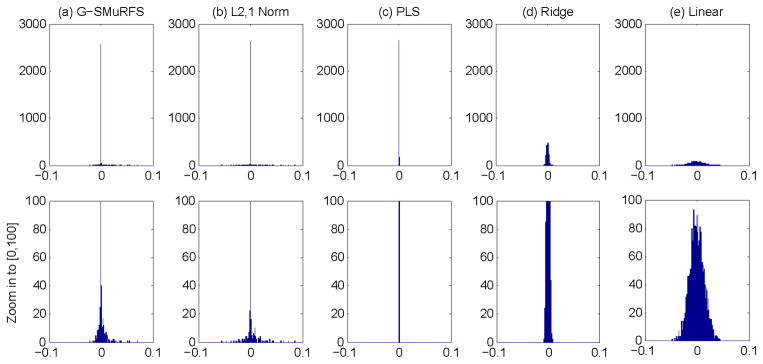
Histogram of regression weights of all cortical measures for predicting the RAVLT TOTAL score in an example cross-validation trial. Shown from left to right are the results of (a) G-SMuRFS, (b) ℓ_2,1-norm, (c) PLS, (d) ridge regression, and (e) linear regression. The top row shows the complete histograms, and the bottom row shows the zoom in view of the partial histograms for y∈[0, 100].

Figure 4.

Cortical map of regression weights for predicting the RAVLT TOTAL score in an example cross-validation trial using five different models: (a) G-SMuRFS, (b) ℓ_2,1-norm, (c) PLS, (d) ridge regression, and (e) linear regression. The red color indicates regions where the thickness is positively correlated with the RAVLT TOTAL score, and the blue color indicates regions where the thickness is negatively correlated with the score. Shown in (f) are 34 pairs of color-coded bilateral cortical ROIs.

Besides the sparsity at the cortical patch level, we also examined the group sparsity of all five models at the ROI level. In Fig. 5, ROI level sparsity is demonstrated through the histogram of “high impact” (i.e., top 50) cortical markers against each of the 34 pairs of bilateral ROIs for (a) G-SMuRFS, (b) ℓ_2,1-norm, (c) PLS, (d) ridge regression, and (e) linear regression respectively. Each vertical bar here indicates an ROI in the brain. While the top 50 biomarkers identified by G-SMuRFS are associated with a small number of ROIs, the same number of high impact biomarkers identified through ℓ_2,1-norm, ridge regression, and linear regression are scattered across a large portion of cortical surface regions, making the result hard to interpret. G-SMuRFS yielded sparse patterns at the ROI level that have the potential for identifying relevant biomarkers. Although PLS also yielded sparse patterns, the predictive power of its top 50 markers (RMSE=1.045, CC=0.377) is lower than that of G-SMuRFS’s (RMSE=0.938, CC=0.46).

Figure 5.

Number of “high impact” (i.e., top 50) cortical markers for predicting the RAVLT TOTAL score, in an example cross-validation trial, is plotted against the corresponding ROI (34 ROIs in total). The x axis shows the ROI IDs (see Table 1 for the corresponding ROI names). The y axis shows the number of top markers in the left hemisphere ROI (top row) or the right hemisphere ROI (bottom row). Shown from left to right are the results of (a) G-SMuRFS, (b) ℓ_2,1-norm, (c) PLS, (d) ridge regression, and (e) linear regression. The cross-validation performance using these top 50 markers, measured by root mean square error (RMSE) and correlation coefficient (CC) between the actual and predicted RAVLT TOTAL scores of all the test subjects, is shown in each panel.

Fig. 6 shows example G-SMuRFS regression weights that were averaged over the five cross-validation trials and were then mapped back onto the cortical surface. Our multi-task regression experiment was performed to identify thickness measures for jointly predicting ADAS, MMSE, RAVLT TOTAL, RAVLT RECOG, and RAVLT T30 scores. The weight maps for ADAS (Fig. 6a), MMSE (Fig. 6b), TOTAL (Fig. 6c), RECOG (Fig. 6d), and T30 (not shown) are very similar to one another except that the ADAS pattern is in the opposition direction. Thickness measures from left and right entorihnal cortex, left middle temporal gyri, left inferior parietal gyri, right medial orbitofrontal gyri, and right precunes are positively correlated to the MMSE and RAVLT scores, and negatively correlated to ADAS. The measures from left fusiform are correlated to ADAS, MMSE, TOTAL and T30, and the measures from right middle temporal gyri are correlated to ADAS, MMSE, and RECOG. These patterns identified by our multivariate G-SMuRFS regression analysis match well with the weight map patterns computed by the univariate SurfStat analysis shown in Fig. 7.

Figure 6.

Example G-SMuRFS regression weights are color-coded and mapped onto the cortical surface. The red color indicates regions where the thickness is positively correlated with the corresponding cognitive score ((a) ADAS, (b) MMSE, (c) RAVLT-TOTAL, or (d) RAVLT-RECOG), and the blue color indicates regions where the thickness is negatively correlated with the score.

Figure 7.

Example SurfStat t-statistic map: t-statistics are color-coded and mapped onto the cortical surface.

The ROIs identified in this work are either related to AD or in accordance with findings in similar prior studies. For example, entorihnal cortex (part of medial temporal cortex) and precuneus are among the cortical signature of AD studied in (Bakkour, et al., 2009, Dickerson, et al., 2009). Wan, et al. (2012), Wan, et al. (2014) and Wang, et al. (2011) performed similar regression studies for predicting cognitive outcomes using MRI measures. However, they examined only summary statistics (volume, thickness, or gray matter density) of both cortical and subcortical ROIs instead of detailed cortical thickness measures. The mean thickness of entorihnal cortex was found to be correlated with ADAS (Wan, et al., 2014), MMSE (Wan, et al., 2014) and RAVLT (Wan, et al., 2014, Wang, et al., 2011) scores. The mean thickness of inferior parietal gyri was found to be correlated with ADAS (Wan, et al., 2014) and RAVLT (Wang, et al., 2011) scores. The mean thickness of middle temporal gyri was found to be correlated with RAVLT scores (Wan, et al., 2012). Partly due to the detailed cortical analysis, this work identified some additional ROIs associated with the studied cognitive scores. Replication of these results in independent samples will remain of critical importance for confirmation.

The computational cost of G-SMuRFS was similar to that of the ℓ_2,1-norm model but more expensive than linear, ridge and PLS regressions. We implemented all the regression models using Matlab. For one cross-validation trial in our experiments, G-SMuRFS and ℓ_2,1-norm took 75–77 seconds while linear regression took 48 seconds, and ridge and PLS took < 2 seconds. One interesting future direction is to develop more efficient implementation of G-SMuRFS and make it applicable to the analysis of larger scale data sets.

To sum up, our empirical results are very encouraging and have demonstrated the promise of the G-SMuRFS method in the application of relating cortical morphology to cognitive outcomes: (1) G-SMuRFS regression model outperformed linear, ridge and PLS regression models, and performed similarly to the multi-task ℓ_2,1-norm model in terms of overall RMSE and CC (Table 3). (2) The biomarkers identified by the G-SMuRFS method were sparser at the patch level than linear regression and ridge regression, and yielded a more stable performance for predicting cognitive scores. (3) Both G-SMuRFS and ℓ_2,1 methods yielded sparse results at the vertex level (Fig. 3 and Fig. 4), however the G-SMuRFS model presented a sparser pattern at the ROI level (Fig. 5) than the ℓ_2,1-norm model. Taking into account the spatial information makes the best use of the detailed surface information, yet leading to a clustered group level result instead, which is more visible and interpretable.

4. Conclusions

We have investigated the power of detailed cortical thickness measurements for predicting ADAS, MMSE and RAVLT cognitive scores using the data from the ADNI cohort. We have proposed to employ a newly developed sparse multi-task learning algorithm called G-SMuRFS, and have observed the following strengths of this approach that could greatly improve the prediction performance: (1) seamless integration of anatomical knowledge in the learning process by coupling cortical measures from the same ROI together; (2) sparsity at both patch level and ROI level; and (3) multitask learning scheme for addressing correlation among response variables.

Compared to Linear, ridge, PLS, or ℓ_2,1-norm regression, combining the group ℓ_2,1-norm in the regularization term has not only helped select the potential biomarkers in a few ROIs, but also improved overall predictive power. Its application to multi-modal imaging data would be promising future directions for biomarker discovery and better mechanistic understanding in AD research. Exploration of other imaging modalities as well as the combination of multiple modalities warrants further investigation. Further effort may be made to include more complicated prior structure, like multiple layer groups or networks, to guide the learning procedure. Another possible future topic could be to investigate whether nonlinear models can help improve the prediction rates as well as derive biologically meaningful results.

Highlights.

• We examine the predictive power of cortical measures towards cognitive scores

• We consider the group structures defined by anatomically meaningful ROIs

• We apply G-SMuRFS to predict cognitive scores using cortical thickness measures

• G-SMuRFS demonstrates a superior prediction performance

• G-SMuRFS identifies a small set of biologically meaningful surface markers

References

- Avants BB, Cook PA, Ungar L, Gee JC, Grossman M. Dementia induces correlated reductions in white matter integrity and cortical thickness: a multivariate neuroimaging study with sparse canonical correlation analysis. NeuroImage. 2010;50(3):1004–16. doi: 10.1016/j.neuroimage.2010.01.041. [DOI] [PMC free article] [PubMed] [Google Scholar]
- Bakkour A, Morris JC, Dickerson BC. The cortical signature of prodromal AD: regional thinning predicts mild AD dementia. Neurology. 2009;72(12):1048–55. doi: 10.1212/01.wnl.0000340981.97664.2f. [DOI] [PMC free article] [PubMed] [Google Scholar]
- Batmanghelich NK, Taskar B, Davatzikos C. Generative-discriminative basis learning for medical imaging. IEEE transactions on medical imaging. 2012;31(1):51–69. doi: 10.1109/TMI.2011.2162961. [DOI] [PMC free article] [PubMed] [Google Scholar]
- Chung MK, Worsley KJ, Nacewicz BM, Dalton KM, Davidson RJ. General multivariate linear modeling of surface shapes using SurfStat. NeuroImage. 2010;53(2):491–505. doi: 10.1016/j.neuroimage.2010.06.032. [DOI] [PMC free article] [PubMed] [Google Scholar]
- Dale AM, Fischl B, Sereno MI. Cortical surface-based analysis. I. Segmentation and surface reconstruction. NeuroImage. 1999;9(2):179–94. doi: 10.1006/nimg.1998.0395. [DOI] [PubMed] [Google Scholar]
- Dickerson BC, Bakkour A, Salat DH, Feczko E, Pacheco J, Greve DN, Grodstein F, Wright CI, Blacker D, Rosas HD, Sperling RA, Atri A, Growdon JH, Hyman BT, Morris JC, Fischl B, Buckner RL. The cortical signature of Alzheimer’s disease: regionally specific cortical thinning relates to symptom severity in very mild to mild AD dementia and is detectable in asymptomatic amyloid-positive individuals. Cereb Cortex. 2009;19(3):497–510. doi: 10.1093/cercor/bhn113. [DOI] [PMC free article] [PubMed] [Google Scholar]
- Fischl B, Sereno MI, Dale AM. Cortical surface-based analysis - II: Inflation, flattening, and a surface-based coordinate system. NeuroImage. 1999;9(2):195–207. doi: 10.1006/nimg.1998.0396. [DOI] [PubMed] [Google Scholar]
- Grosenick L, Klingenberg B, Katovich K, Knutson B, Taylor JE. Interpretable whole-brain prediction analysis with GraphNet. NeuroImage. 2013;72:304–21. doi: 10.1016/j.neuroimage.2012.12.062. [DOI] [PubMed] [Google Scholar]
- Jenatton R, Gramfort A, Michel V, Obozinski G, Eger E, Bach F, Thirion B. Multiscale Mining of fMRI Data with Hierarchical Structured Sparsity. SIAM Journal on Imaging Sciences. 2012;5(3):835–56. doi: 10.1137/110832380. [DOI] [Google Scholar]
- Michel V, Gramfort A, Varoquaux G, Eger E, Thirion B. Total variation regularization for fMRI-based prediction of behavior. IEEE transactions on medical imaging. 2011;30(7):1328–40. doi: 10.1109/TMI.2011.2113378. [DOI] [PMC free article] [PubMed] [Google Scholar]
- Puniyani K, Kim S, Xing EP. Multi-population GWA mapping via multi-task regularized regression. Bioinformatics. 2010;26(12):i208–16. doi: 10.1093/bioinformatics/btq191. [DOI] [PMC free article] [PubMed] [Google Scholar]
- Sabuncu MR, Van Leemput K. The relevance voxel machine (RVoxM): a self-tuning Bayesian model for informative image-based prediction. IEEE transactions on medical imaging. 2012;31(12):2290–306. doi: 10.1109/TMI.2012.2216543. [DOI] [PMC free article] [PubMed] [Google Scholar]
- Saykin AJ, Shen L, Foroud TM, Potkin SG, Swaminathan S, Kim S, Risacher SL, Nho K, Huentelman MJ, Craig DW, Thompson PM, Stein JL, Moore JH, Farrer LA, Green RC, Bertram L, Jack CR, Jr, Weiner MW. Alzheimer’s Disease Neuroimaging Initiative biomarkers as quantitative phenotypes: Genetics core aims, progress, and plans. Alzheimers Dement. 2010;6(3):265–73. doi: 10.1016/j.jalz.2010.03.013. [DOI] [PMC free article] [PubMed] [Google Scholar]
- Shen L, Kim S, Risacher SL, Nho K, Swaminathan S, West JD, Foroud T, Pankratz N, Moore JH, Sloan CD, Huentelman MJ, Craig DW, Dechairo BM, Potkin SG, Jack CR, Jr, Weiner MW, Saykin AJ. Whole genome association study of brain-wide imaging phenotypes for identifying quantitative trait loci in MCI and AD: A study of the ADNI cohort. NeuroImage. 2010;53(3):1051–63. doi: 10.1016/j.neuroimage.2010.01.042. [DOI] [PMC free article] [PubMed] [Google Scholar]
- Tibshirani R. Regression shrinkage and selection via the lasso. J R Stat Soc Ser B. 1996;58:267–288. [Google Scholar]
- Varoquaux G, Gramfort A, Thirion B. Small-sample brain mapping: sparse recovery on spatially correlated designs with randomization and clustering. ICML. 2012;2012 [Google Scholar]
- Wagner AD, Shannon BJ, Kahn I, Buckner RL. Parietal lobe contributions to episodic memory retrieval. Trends in cognitive sciences. 2005;9(9):445–53. doi: 10.1016/j.tics.2005.07.001. [DOI] [PubMed] [Google Scholar]
- Wan J, Zhang Z, Rao B, Fang S, Yan J, Saykin A, Shen L. Identifying the Neuroanatomical Basis of Cognitive Impairment in Alzheimer’s Disease by Correlation- and Nonlinearity-Aware Sparse Bayesian Learning. IEEE transactions on medical imaging. 2014 doi: 10.1109/TMI.2014.2314712.. [DOI] [PMC free article] [PubMed] [Google Scholar]
- Wan J, Zhang Z, Yan J, Li T, Rao B, Fang S, Kim S, Risacher S, Saykin A, Shen L ADNI ft. Sparse Bayesian multi-task learning for predicting cognitive outcomes from neuroimaging measures in Alzheimer’s disease. CVPR’12: IEEE Int Conf on Computer Vision and Pattern Recognition, Providence; Rhode Island. 2012. [Google Scholar]
- Wang H, Nie F, Huang H, Kim S, Nho K, Risacher S, Saykin A, Shen L. Identifying quantitative trait loci via group-sparse multi-task regression and feature selection: An imaging genetics study of the ADNI cohort. Bioinformatics. 2012;28(2):229–37. doi: 10.1093/bioinformatics/btr649. [DOI] [PMC free article] [PubMed] [Google Scholar]
- Wang H, Nie F, Huang H, Risacher S, Ding C, Saykin A, Shen L. Sparse multi-task regression and feature selection to identify brain imaging predictors for memory performance. IEEE Conference on Computer Vision; Barcelona, Spain. 2011. pp. 557–62. [DOI] [PMC free article] [PubMed] [Google Scholar]
- Weiner MW, Aisen PS, Jack CR, Jr, Jagust WJ, Trojanowski JQ, Shaw L, Saykin AJ, Morris JC, Cairns N, Beckett LA, Toga A, Green R, Walter S, Soares H, Snyder P, Siemers E, Potter W, Cole PE, Schmidt M. The Alzheimer’s disease neuroimaging initiative: progress report and future plans. Alzheimers Dement. 2010;6(3):202–11. e7. doi: 10.1016/j.jalz.2010.03.007. [DOI] [PMC free article] [PubMed] [Google Scholar]
- Yuan M, Lin Y. Model selection and estimation in regression with grouped variables. J R Stat Soc Ser B. 2006;68:49–67. [Google Scholar]