

Abstract
The brain connectome collects the complex network architectures, looking at both static and dynamic functional connectivity. The former normally requires stationary signals and connections. However, the human brain activity and connections are most likely time dependent and dynamic, and related to ongoing rhythmic activity. We developed an open-source MATLAB toolbox DynamicBC with user-friendly graphical user interfaces, implementing both dynamic functional and effective connectivity for tracking brain dynamics from functional MRI. We provided two strategies for dynamic analysis: (1) the commonly utilized sliding-window analysis and (2) the flexible least squares based time-varying parameter regression strategy. The toolbox also implements multiple functional measures including seed-to-voxel analysis, region of interest (ROI)-to-ROI analysis, and voxel-to-voxel analysis. We describe the principles of the implemented algorithms, and then present representative results from simulations and empirical data applications. We believe that this toolbox will help neuroscientists and neurologists to easily map dynamic brain connectomics.
Key words: : brain connectome, dynamic, effective connectivity, functional connectivity, resting-state fMRI
Introduction
The brain connectome collects network architectures. At macroscopic scales, the human brain connectomics provide a comprehensive description of the anatomical pathways and functional interactions among distinct brain areas (Sporns, 2013, 2014). The structural connectomics essentially comprises a comprehensive map of the anatomical connections reflecting axonal pathways (Sporns et al., 2005), and the structural covariance connectivity interpreted as the phenotype of brain development and/or plasticity (Alexander-Bloch et al., 2013; He et al., 2007). Additionally, the functional connectomics can be captured as patterns of functional covariance network (Liao et al., 2013b; Zhang et al., 2011), functional connectivity (FC) and effective connectivity (EC) networks (Friston, 2009, 2011; Marinazzo et al., 2011, 2014; Wu et al., 2013b).
FC measures statistical patterns of interactions among remote brain regions; while EC discerns the transfer of information such as directed causal interactions (Friston, 1994; Rubinov and Sporns, 2010). Consequently, the brain can be seen as a large-scale functional integrated network both during cognitive tasks and at resting state (Bressler and Menon, 2010). Resting-state FC represents the synchronization of spontaneous blood-oxygenation level-dependent (BOLD) activity and is typically analyzed in terms of correlation, coherence, and spatial grouping based on temporal similarities (Beckmann et al., 2005; Biswal et al., 1995; van den Heuvel et al., 2008). These FC analyses always assume that the functional connections remain constant during the whole period of data collection.
However, both emerging theoretical ideas and empirical observations suggest that the human brain connectome is most likely to be time dependent and dynamic, and to be related to ongoing rhythmic activity (Sporns, 2011). The functional repertoire of brain connectome is continually revisited and rehearsed in endogenous neural activity (Deco and Corbetta, 2011). Recent empirical human, macaque, and rat studies have observed the phenomenon that brain FC can indeed exhibit nonstationary activity, and change over a short time (Allen et al., 2014; Chang and Glover, 2010; de Pasquale et al., 2010; Di and Biswal, 2013; Handwerker et al., 2012; Hutchison et al., 2013b; Kang et al., 2011; Lee et al., 2013), and even across a few spontaneous points (Liu and Duyn, 2013; Tagliazucchi et al., 2012a; Wu et al., 2013a). Hence, dynamic techniques track the variability of the topology of the brain connectome across different cognitive states (Bassett et al., 2011; Fornito et al., 2012) and the evolution of diseased brain networks (Liao et al., 2013a; Zhang et al., 2014).
Several modeling strategies have been developed to meet brain dynamics' need (Hutchison et al., 2013a). The most commonly utilized approach, called sliding-window analysis, is performed by conducting FC on a set number of data points. Much earlier defined paradigms information or stationary assumptions regarding the signal must be made prior to its calculation. Another widely used data-driven approach, such as Kalman filtering (KF), is capable of assessing rapidly changing connectivity relationships between brain areas (Kang et al., 2011).
Recently, several advanced toolboxes providing indexes of dynamic brain connectivity have been developed, such as GIFT (http://mialab.mrn.org/software/gift/) (Allen et al., 2014), eConnectome (http://econnectome.umn.edu) (He et al., 2011), and BSMART (www.brain-smart.org/) (Cui et al., 2008). However, most of them either focus on a special modality (e.g., functional magnetic resonance imaging [fMRI], electroencephalography [EEG], magnetoencephalography) and/or include only a subset of measures as part of a more general-purpose toolbox. More important, tracking dynamic FC (d-FC) and dynamic EC (d-EC) extends the repertoire of brain connectome. However, it is still desired that a unified toolbox facilitate the neuroscientist and neurologist to easily map dynamic brain connectome.
We hereby developed a publicly available toolbox named DynamicBC (dynamic brain connectome toolbox; www.restfmri.net/forum/DynamicBC). It is an open-source MATLAB toolbox with user-friendly graphical user interfaces (GUI). The toolbox supports NIfTI and ANALYZE images (*.nii and *.img) that would be preprocessed in the REST (Song et al., 2011) and the DPARSF (Chao-Gan and Yu-Feng, 2010) toolkit, in addition to ASCII and .mat formats. The DynamicBC implements both d-FC and d-EC for tracking brain dynamics from fMRI. Particularly, a distribution-free time-varying parameter regression strategy was implemented. In addition, multiple region of interest (ROI) setting ways are provided, for example, seed-to-voxel, ROI-to-ROI and voxel-to-voxel. In the following section, the remainder of this work first describes the principles of the algorithms implemented, and then we present representative results from simulations and real data, to illustrate the reliability of all these dynamic connectivity measures.
Function Module Implemented in DynamicBC
Overview of usage of the toolbox
The DynamicBC was developed by cross platform MATLAB (Mathworks, Inc.) programming language, with a user-friendly GUI, under a 64-bit Windows environment. It is integrated by the modules of connectivity types, dynamic analysis strategies, and ROI set (Fig. 1).
FIG. 1.

The framework of the DynamicBC toolbox. A graphical user interface (GUI) can be started by calling the “DynamicBC'” function in the command window of the MATLAB. The following procedures include three parts: the selection of connectivity types (the functional connectivity [FC] and effective connectivity [EC]), selection of dynamic analysis strategies (the sliding-window and flexible least squares [FLS]), and selection of connectivity measures (the seed-to-voxel, region of interest [ROI]-to-ROI, and voxel-to-voxel analysis). The subsequent brain connectomes are then visualized. Color images available online at www.liebertpub.com/brain
Connectivity types selection
Functional connectivity
The toolbox focuses on the Pearson linear correlation to measure the FC between pair of regions:
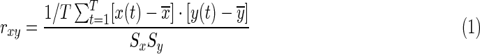 |
where rxy is the Pearson correlation coefficient, x(t) and y(t) are the seed and target variables with means  and
and  , and standard deviations Sx and Sy, respectively. The summation limit, T, corresponds to the total number of time points. The most resting-state fMRI studies used this Pearson linear correlation with full-length time series, referred to as static FC (s-FC) (Biswal et al., 1995; Fox et al., 2005; Fransson, 2005; Zuo et al., 2012).
Effective connectivity
The bivariate Granger causality (GC) to explore EC was employed in the current toolbox, which tested the null hypothesis that region x does not Granger-cause region y measured via linear autoregressive model. The GC index from x to y is defined as follows:
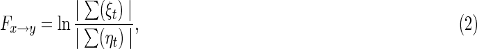 |
where ξt and ηt are the residuals of the restricted and unrestricted regression models respectively, and ∑ indicates the variance. The static EC (s-EC) was termed to describe GC relationship by full-length time series.
Dynamic analysis strategies
To describe the dynamic connectivity among the brain areas, we employed a time-varying parameter regression method, which is briefly described as follows:
 |
where x(t) and y(t) are the seed and target variables respectively, and u(t) is the approximation error, and β(t) is the coefficient to determine whether two variables covary and reflect the dynamic connectivity between x and y at time t.
Sliding-window analysis
If we treat x and y in a short time window as being generated by an underlying (approximately) and stationary stochastic process, then the model has constant parameters during this short period. Furthermore, if the values of x and y are normally distributed and homoscedastic, coefficient 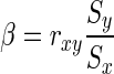 can be estimated by ordinary least squares estimate in a short time window. Here, we employ rxy as the strength of d-FC in the short time window, without considering of the scaling in samples. By transforming equation (3) into the vector autoregressive model, and following a similar procedure, the time-varying GC between x and y could be evaluated by means of sliding-window analysis.
Flexible least squares
The value of β(t) may continuously change for various reasons. For example, switching in different tasks, or could be the consequence of underlying physiological process. There are two approaches to estimate the continuous changed model parameters at each observation. One popular methodology is the application of the KF to infer time-varying parameters (Kalman, 1960). Another tool is the flexible least squares (FLS) (Hastie and Tibshirani, 1993; Kalaba and Tesfatsion, 1989). The KF typically builds on the assumption of a certain distribution in the innovations (which is usually set to be normal distribution), while FLS is distribution-free. Here, we only focus on the distribution-free method. The idea of the FLS method is to assign two types of residual error to each possible coefficient sequence estimate. The first one is the sum of squared residual measurement errors:
 |
matching the prior measurement specification: y(t) − x(t) β(t)≈0. The other is the sum of squared residual dynamic error, in which FLS declares that the vector of coefficients evolves slowly over time (β(t+1) − β(t)≈0), formally:
 |
with a given μ weighting parameter, Kalaba and Tesfatsion (Kalaba and Tesfatsion, 1989) define the incompatibility cost assigned to any β coefficient sequence as
 |
The incompatibility cost function C(β, μ, T) generalizes the goodness-of-fit criterion function for ordinary least squares estimation by permitting the coefficient vector β(t) to vary over time. When μ approaches was set to zero,  can generally be brought down close to zero and the corresponding value for
  will be relatively large, resulting in a rather erratic sequence of estimates. As μ becomes arbitrarily large, the incompatibility cost function assigns all importance to the dynamic specification. This case yields the ordinary least squares solution,
  is minimized subject to the following formula:
  .
.
ROI set for d-FC and d-EC
The implementation includes three ways to set ROI for dynamic brain connectivity analysis (Fig. 1). Seed-to-voxel (voxel wise) analysis calculated the bivariate FC/EC between seed brain region and every voxel in the whole brain. ROI-to-ROI (ROI-wise) analysis computed the bivariate FC/EC between each pair of ROIs, resulting brain connectivity matrix (network) allows users to further perform graph theoretical analysis (Liao et al., 2010; Wu et al., 2013b). Voxel-to-voxel computed the bivariate FC/EC between every pair of voxels without using a priori seed/ROI to mapping whole-brain connectome (Tomasi and Volkow, 2010; Zuo et al., 2012). In addition, the toolbox then provides the FC degree that counts total number of connections of a given voxel, while the FC/EC strength (FCS/ECS) that sums of weights of all the connections of a given voxel. Only FC/EC value of given voxel above a predefined threshold (corresponding p-value or family-wise error corrected p-value) were counted or summed.
Illustrations of Dynamic Brain Connectome
Simulation
The following simulated example is explored here to validate the reliability of uncovering d-FC by short sliding-window analysis and FLS, and the KF analysis were included.
where ɛ and ɛi follow a normal distribution with mean 0 and variance 0.3. The generated data of y and xi are shown in Figure 2A. The FC between y and xi are evaluated by s-FC and d-FC [included sliding-window analysis (window size=20 time points, step=1 time point), FLS (μ=20), and KF with default parameters (Peng and Aston, 2011)]; the s-FC and d-FC by sliding widow method is drawn as the pink and green line, respectively. The yellow filled area indicates the 95% confidence intervals for β coefficient (red line) estimated by KF method (Fig. 2B, C), and there is no significant connectivity between the two signals at a time point when the enclosed range did not cover zero; the overlapped blue line is β estimated by FLS method. These results suggest that both the FLS and sliding window analysis could capture ground truth β over time. Under the different parameters, sliding window analysis and FLS may induce different results, experimental outcomes of FLS for μ=0.01, 0.1, 1, 10, 100, 1000, and 1000 are plotted in Figure 3.
FIG. 2.

The simulated data and dynamic interactions. (A) Signals are generated according to equation (7). The blue, green, and red lines denote signals x1, x2, and y, respectively. They are normalized to a mean=0 and a variance=0.3. (B, C) The static FC (s-FC) and dynamic FC (d-FC) by sliding-window analysis is drawn as the peach-puff and green line, respectively. The 95% confidence intervals for β coefficient (red line) estimated by the Kalman filtering (KF) method is shown as the yellow-filled area, and the blue line indicated β estimated by the FLS method. Color images available online at www.liebertpub.com/brain
FIG. 3.

The differential β amplitudes as estimated by the FLS method with different penalty weights μ, which increase by powers of ten: 0.01, 0.10, 1, 10, 100, 1000, and 10,000. The gray line indicates the ground truth β. Color images available online at www.liebertpub.com/brain
fMRI data
We selected 32 young healthy subjects (10 females, all right-handed; age: 25.19±6.71 years) from our previous studies (Liao et al., 2013b; Zhang et al., 2011). The subjects had no history of neurological disorder or psychiatric illness and no gross abnormalities in the brain MRI images. Written informed consent was obtained from all subjects. The study was approved by the Local Medical Ethics Committee at Jinling Hospital, Nanjing University School of Medicine.
We performed functional neuroimaging acquisitions using a Siemens Trio 3T scanner at Jinling Hospital. We used foam padding to minimize head motion. We acquired resting-state functional images using a single-shot, gradient-recalled echo planar imaging sequence (250 volumes, repetition time=2000 msec, echo time=30 msec, flip angle=90°, field of view=240×240 mm2, inter-slice gap=0.4 mm, voxel size=3.75×3.75×4 mm3, 30 transverse slices aligned along the anterior–posterior commissure). Subjects were instructed simply to rest with their eyes closed, not to think of anything in particular, and not to fall asleep. Subsequently, we acquired 3D T1-weighed anatomical images in sagittal orientation using a magnetization-prepared rapid gradient-echo sequence (repetition time=2300 msec, echo time=2.98 msec, flip angle=9°, field of view=256×256 mm2, voxel size=0.5×0.5×1 mm3, 176 slices without inter-slice gap).

Preprocessing
Functional images were preprocessed using the REST (Song et al., 2011), DPARSF (www.restfmri.net) (Chao-Gan and Yu-Feng, 2010) and SPM8 (www.fil.ion.ucl.ac.uk/spm) toolkits. We excluded the first 10 images to ensure steady state longitudinal magnetization, and then we corrected the remaining images for temporal differences and head motion. No translation or rotation parameters in any given data set exceeded ±1 mm or ±1°. The individual 3D T1-weighted anatomical image was coregistered to the functional images. The 3D T1-weighted anatomical images were segmented (gray matter, white matter, and cerebrospinal fluid). A nonlinear spatial deformation was then calculated from the gray matter images to a gray matter template in Montreal Neurological Institute (MNI) space using 12 parameters that were defined by affine linear transformation. This transformation was then applied to the functional images. The normalized images were resliced at a resolution of 3×3×3 mm3. Nine sources of variances including six head motion parameters, averaged signals from cerebrospinal fluid and white matter, and global brain signal were regressed. Next, the data were band-pass filtered (0.01–0.08 Hz).
Seed-to-voxel-based s-FC and d-FC patterns
For seed-to-voxel analysis, a sphere (radius=6 mm) in the posterior cingulate cortex (PCC; MNI coordinates: −2, −48, 28) was defined as the seed according to previous study (Spreng et al., 2013). The averaged BOLD time series was then obtained from the PCC and linear Pearson correlation analysis was performed in a voxel-wise way using full-length time series to generate s-FC map. Next, the s-FC map of each subject was converted into z map by Fisher's z transformation. Finally, z maps were combined across subjects using a fixed-effects analysis (sum and divided by the square root of number of subjects) to generation group s-FC map. The s-FC pattern was consistent with previous resting-state fcMRI studies (Fig. 4A) (Fox et al., 2005; Fransson, 2005; Zhang et al., 2011). The PCC showed positive s-FC with medial prefrontal cortex (mPFC), bilateral inferior parietal lobule, middle temporal gyrus, and superior frontal gyrus. These regions are considered part of the default mode network (DMN) (Raichle et al., 2001). In addition, the PCC showed negative s-FC with brain regions involving the frontoparietal control network (FPCN), and the dorsal attention network (DAN).
FIG. 4.

Illustration of the seed-to-voxel-wise s-FC and d-FC. (A) Group-averaged s-FC map following the linear Pearson's correlation analysis using the full-length of the resting-state blood-oxygenation level-dependent (BOLD) functional magnetic resonance imaging (fMRI) signal with a seed placed in the posterior cingulate cortex (PCC; Montreal Neurological Institute [MNI] coordinates: −2, −48, 28, 6 mm radius sphere). (B) d-FC map following FLS analysis with the PCC seed of a representative healthy subject. Two target ROIs with a 6 mm radius sphere were placed in the medial prefrontal cortex (mPFC, MNI coordinates: 6, 51, 9), and right superior parietal lobule (SPL, MNI coordinates: 63, −33, 39). The d-FC (solid line) and s-FC (dashed line) time series of mPFC (red line) and SPL (blue line) varied in a time-dependent manner. Warm and cool colors indicate brain regions with positive and negative temporal correlations with the PCC seed, respectively. Color scales represent the group-averaged correlation coefficient value (Z) of the s-FC map and individual β amplitude values of the d-FC map, respectively. See Supplementary Movie S1; Supplementary Data are available online at www.liebertpub.com/brain Color images available online at www.liebertpub.com/brain
The above-mentioned PCC seed was also applied to d-FC analysis. The FLS analysis strategy was selected for illustrating here. d-FC organizations of one representative subject are shown in Figure 4B (see corresponding Supplementary Movie S1; Supplementary Data are available online at www.liebertpub.com/brain). To display PCC seeded FC dynamics, two target ROIs with 6 mm radius sphere (mPFC, MNI coordinates: [6, 51, 9], and superior parietal lobule [SPL], MNI coordinates: [63, −33, 39]) were identified in s-FC map (Fig. 4A). As seen from d-FC time series, FC between the PCC seed and the mPFC target, which both are belongs to the DMN, is relatively stable (solid red line); while FC between the PCC seed and SPL target involved in the DAN is highly nonstationary (solid blue line), in some cases exhibiting both strongly negative and correlations within the whole scan. These results give an evidence that the FC between brain regions has more variable in distinct networks than within one network (Allen et al., 2014).
Seed-to-voxel-based s-EC and d-EC patterns
For s-EC and d-EC analysis, we also defined the PCC as seed (see Seed-to-voxel-based s-FC and d-FC patterns section). The averaged PCC BOLD time series was used to compute the GCA value of each voxel using full-length time series, resulting in s-EC map. Then, the s-EC map of each subject was combined across subjects using a fixed-effects analysis to generation group s-EC map. The s-EC from the PCC to whole brain (“out” map) and whole brain to PCC (“in” map) were illustrated in Figure 5A.
FIG. 5.

Illustration for seed-to-voxel-wise static EC (s-EC) and dynamic EC (d-EC). (A) Group-averaged s-EC map following linear residual-based Granger causality analysis (GCA) using full length of resting-state BOLD fMRI signal with a seed placed in the PCC (MNI coordinates: −2, −48, 28, 6 mm radius sphere). (B) d-EC map following sliding-window analysis of linear residual-based GCA with the PCC seed of a representative healthy subject. One target ROI with 6 mm radius sphere placed in the mPFC (MNI coordinates: 3, 39, 18). The d-EC (solid line) and s-EC (dashed line) time series of mPFC from the in map (red line) and out map (blue line) vary across time. Warm and cool colors indicate brain regions with in influence (from whole brain to the seed) and out influence (from seed to whole brain), respectively. Color scales represent group-averaged GC value (F) of s-EC map and individual β amplitude values of d-EC map, respectively. See Supplementary Movies S2 and S3. Color images available online at www.liebertpub.com/brain
Subsequently, we evaluated d-EC using the sliding-window GC analysis. We calculated GC maps between the PCC time series and all other brain voxel for a sliding-window of 50 volumes. For each sliding-window, we obtained the GC value in and out maps. The window was then shifted by 5 volumes and a new GC maps was calculated. This analysis strategy permitted to estimate d-EC over time. The d-EC map showing GC from whole brain to the PCC (upper panel) and from the PCC to whole brain (bottom panel) are illustrated as in Figure 5B (see Supplementary Movies S2 and S3). As see from d-EC time series of the target region mPFC, both the in- and out-influence are relatively stable and consistent changes across time.
ROI-to-ROI-based s-FC and d-FC networks
To illustrate the ROI-to-ROI-based d-FC networks, we selected 43 ROIs, which are involved in the DMN, DAN, and FPCN in line with the previous study (Spreng et al., 2013). Detailed brain regions and corresponding MNI coordinates and abbreviations of each ROI are shown in Supplementary Table S1. We extracted the averaged BOLD time series from the each ROI (6 mm radius sphere) from each subject.
We computed the Pearson linear correlation coefficient between a pair of ROIs using the full length of the time series, and the square 43×43 s-FC matrix was obtained individually. Then, s-FC matrices after Fisher's z transformation were combined across subjects using a fixed-effects analysis to generation group s-FC matrix. To visualize the s-FC network, we positioned the regional centroid of each ROI (node) according to its MNI coordinates, and defined the threshold (p<0.01, Bonferroni corrected) to remove spurious connection (edge). Node strength was computed as the sum of the weights of all the connections of a given ROI. Finally, s-FC network was visualized using the BrainNet Viewer (www.nitrc.org/projects/bnv/) (Xia et al., 2013) (Fig. 6A). We observed that a high degree of integration within each sub-network and anticorrelation between the DMN and the DAN and FPCN. The PCC and mPFC exhibited the high node strength, considering as core hubs. These findings are consistent with the previous studies (Fox et al., 2005; Spreng et al., 2013).
FIG. 6.

Illustration for ROI-to-ROI wise s-FC and d-FC. (A) Group-averaged pairwise correlation matrix (upper panel) following linear Pearson correlation analysis using full length of resting-state BOLD fMRI signals from 43 ROIs. This correlation matrix was visualized by brain network (bottom panel). (B) Dynamic functional correlation matrix (upper panel) and brain network (bottom panel) following FLS analysis among pairwise ROIs of a representative healthy subject. The d-FC (solid line) and s-FC (dashed line) time series between the PCC and other three ROIs vary across time. Warm and cool colors in correlation matrix indicate positive and negative correlations, respectively. See Supplementary Movie S4. Color images available online at www.liebertpub.com/brain
For d-FC analysis, the FLS analysis strategy was also used. d-FC network organizations of one representative subject are shown in Figure 6B (see Supplementary Movie S4). As seen from d-FC network dynamics, the fundamental organization, that is integration within network and fractionation between networks, is relatively stable across time (Fig. 6B, upper panel). However, the hub with high regional weights changed hands several times (Fig. 6B, bottom panel), suggesting greater FC variability in the hub for the cognitive process switch. To examine the FC dynamics of core hub PCC, we selected three target ROIs. They are left posterior inferior parietal lobule (pIPL.L), right middle temporal motion complex (MT.R), and right dorsolateral prefrontal cortex (dlPFC.R) in the DMN, DAN, and FPCN, respectively. As seen from the d-FC time series, connectivity between the PCC and pIPL.L (solid red line) is less nonstationary; while that between the PCC and MT.R and between the PCC and dlPFC.R is relatively high nonstationary. This d-FC finding would suggest that some brain regions reveal dual-aligned properties (Spreng et al., 2013).
Voxel-to-voxel-based FC network evolved with absence seizures
Quantification of disrupted dynamical connectome in diseased brain would better understand the evolution of disorder. In the current work, we aimed to observe the transition of whole brain connectome that account for absence seizure onset and offset. To this end, the voxel-to-voxel-based d-FC network was constructed for a representative patient with absence epilepsy.
The patient underwent simultaneous EEG-fMRI session by an MR-compatible EEG recording system (Brain Products). During fMRI acquisition, EEG data were continuously recorded through a 10/20 systems with 32 Ag/AgCl electrodes attached to the scalp with conductive cream. EEG electrodes were connected to a BrainAmp amplifier, with a sampling rate of 5 kHz. The EEG data were processed offline to filter out MR artifacts and remove ballistocardiogram artifacts (Brain Vision Analyzer 2.0). Onset and end time of epileptic discharges were marked and classified according to both spatial distribution and morphology. For more detail about the EEG dataset, see our previous studies (Liao et al., 2013a; Zhang et al., 2014). The resting-state fMRI data of patient with absence epilepsy were preprocessed in line with the healthy subject, except to re-sliced at a resolution of 6×6×6 mm3 to minimize storage and computational requirements. Voxel-to-voxel analysis computed the bivariate FC between every pair of voxels without using a priori seed/ROI. We used the FLS analysis strategy here. In this case, we obtained the FCS maps for each time points as shown in Figure 7 (see Supplementary Movie S5). According to information from simultaneously collected EEG data, the FCS maps were separated into preictal (time before seizure onset), ictal, and postictal (time after seizure end) time periods (Liao et al., 2013a). As previously suggested, the thalamus and PCC were involved in seizure initiation, maintenance, and termination during absence seizures. We selected these two core brain regions as the ROIs to track the FCS dynamics. As seen from d-FCS network dynamics, there is a higher FCS of the thalamus (THA) during the ictal period relative to the periods before and after seizures (blue line). Conversely, the PCC d-FCS time series are lower during the ictal period (red line). These findings suggest that the total connections of thalamus and the PCC relate to mechanisms of seizure generation and suspension of default mode of brain function is consistent with an inhibitory effect of seizures on the default mode of brain function, respectively.
FIG. 7.

d-FC strength (d-FCS). We calculated the d-FCS using FLS analysis strategy of pairwise voxels of a representative patient with absence epilepsy. The yellow shadow indicates ictal period marked by simultaneously collected electroencephalography data. The d-FCS time series of the PCC (red line) and thalamus (THA; blue line) vary preictal, ictal, and postictal periods. See Supplementary Movie S5. Color images available online at www.liebertpub.com/brain
Discussion
We have presented the DynamicBC, a new MATLAB toolbox for the analysis of dynamic brain connectome from multiple functional neuroimaging. In contrast to now available toolboxes, such as, GIFT (Allen et al., 2014), eConnectome (He et al., 2011), BSMART (Cui et al., 2008), and Conn (Whitfield-Gabrieli and Nieto-Castanon, 2012), we now understand that the DynamicBC encompasses both d-FC and d-EC indexes. The aim of the toolbox is to develop a user-friendly GUI for accessibly, and to analyze more comfortably the dynamic brain connectome in which a task or stimulus responses and spontaneous brain activity are measured. To our knowledge, the voxel-level whole brain (GC density/strength) index is firstly available in this toolbox, which could be used to identify the hub of incoming and outgoing information transferring (Wu et al., 2013b).
Particularly, in the current work, we employ FLS algorithm for uncovering the time-varying coefficients of a regression model. Comparing to sliding-window strategy in which the window length is hard to priori define to statistical validation (Hutchison et al., 2013a), the FLS algorithm is a data-driven approach to rapidly assess connectivity changes. In addition, the well-known methodology KF will be added to obtain a comparable result of the transient dynamics (Kang et al., 2011). Meanwhile, FLS and KF model based d-EC algorithms will provide new options to capture the dynamic connectomes.
The present toolbox not only illuminate how much d-FC varies over a scan, but also provide whether the range of d-FC time series variability is significantly different between two populations or between particular regions. The formal group comparisons are challenge for dynamic brain connectome, due to the multi temporal-dimensional nature of the outputs (Hutchison et al., 2013a). According to previous studies, we presented two ways for group analysis. The first sophisticated one, clustering method, collapse the temporal dimension of dynamic connectivity maps/matrices into several outputs or a single one (Allen et al., 2014; Liu and Duyn, 2013). Then, we could perform routine statistical tests between one or more conditions. The second simple one, the variance of the d-FC/d-EC time series (as a proxy of how “stable” a connection is) was calculated automatically. This quantification of dynamic brain connectivity would lead to an improved understanding of the physiological processes of the intact brain or neuropathologic mechanism of the diseased brain.
Another issue related with the recovery of EC networks from BOLD fMRI signal is the possibly confounding effect of the hemodynamic response. To decouple the neuronal activity and the hemodynamic responses, we suggest applying a blind deconvolution procedure, based on the detection of pseudo-events, to the BOLD fMRI signal (Wu et al., 2013a). This blind deconvolution codes have been released and freely available at http://software.incf.org/software/blind-hrf-retrieval-and-deconvolution-for-resting-state-bold.
There are some future directions for the toolbox. Only bivariate dynamic connectivity index are implemented. First, the multivariate or blockwise connectivity measures (Wu et al., 2011) will be integrated in future releases of the tool. Second, implementation of point process event-related nonstationary dynamics of spontaneous activity would be desirable (Tagliazucchi et al., 2012a; Wu et al., 2013a). Third, combining the different EEG rhythms covary with fMRI connectivity over time (Chang et al., 2013; Tagliazucchi et al., 2012b) will be implemented in the future in the toolbox. Finally, we will add a visualization module for dynamic connectome movie.
Conclusion
The DynamicBC toolbox offers a user-friendly and integrated framework to tracking brain connectome by FC and EC. We provide two brain dynamic analysis strategies and three ways to set connections measures. The illustrative results showed the dynamics of FC patters or network in healthy brain and the whole brain connectome evolved with absence seizures. The current version is freely available at www.restfmri.net/forum/DynamicBC. Users would raise questions and give comments by email (dynamicbrainconn@gmail.com) and online forum (www.restfmri.net/forum/). We hope that this toolbox would make the dynamic brain connectome technique easier to develop, and the clinicians will be benefited from the contribution of the toolbox.
Supplementary Material
Acknowledgments
This research was supported by the Natural Science Foundation of China (Grant nos. 81201155 to W.L., 81271553 to Z.Z., and 81020108022 to Y.F.Z), the Grants for Young Scholar in Jinling Hospital (Grant nos. Q2008063, 2011060 to Z.Z), the Qian Jiang Distinguished Professor program to Y.F.Z., the China Postdoctoral Science Foundation (Grant no. 2013 M532229 to W.L., and the Fundamental Research Funds for the Central Universities (Grant No. 2362014xk04 to G.R.W.).
Author Disclosure Statement
No competing financial interests exist.
References
- Alexander-Bloch A, Giedd JN, Bullmore E. 2013. Imaging structural co-variance between human brain regions. Nat Rev Neurosci 14:322–336 [DOI] [PMC free article] [PubMed] [Google Scholar]
- Allen EA, Damaraju E, Plis SM, Erhardt EB, Eichele T, Calhoun VD. 2014. Tracking whole-brain connectivity dynamics in the resting state. Cereb Cortex 24:663–676 [DOI] [PMC free article] [PubMed] [Google Scholar]
- Bassett DS, Wymbs NF, Porter MA, Mucha PJ, Carlson JM, Grafton ST. 2011. Dynamic reconfiguration of human brain networks during learning. Proc Natl Acad Sci U S A 108:7641–7646 [DOI] [PMC free article] [PubMed] [Google Scholar]
- Beckmann CF, DeLuca M, Devlin JT, Smith SM. 2005. Investigations into resting-state connectivity using independent component analysis. Philos Trans R Soc Lond B Biol Sci 360:1001–1013 [DOI] [PMC free article] [PubMed] [Google Scholar]
- Biswal B, Yetkin FZ, Haughton VM, Hyde JS. 1995. Functional connectivity in the motor cortex of resting human brain using echo-planar MRI. Magn Reson Med 34:537–541 [DOI] [PubMed] [Google Scholar]
- Bressler SL, Menon V. 2010. Large-scale brain networks in cognition: emerging methods and principles. Trends Cogn Sci 14:277–290 [DOI] [PubMed] [Google Scholar]
- Chang C, Glover GH. 2010. Time-frequency dynamics of resting-state brain connectivity measured with fMRI. Neuroimage 50:81–98 [DOI] [PMC free article] [PubMed] [Google Scholar]
- Chang C, Liu Z, Chen MC, Liu X, Duyn JH. 2013. EEG correlates of time-varying BOLD functional connectivity. Neuroimage 72:227–236 [DOI] [PMC free article] [PubMed] [Google Scholar]
- Chao-Gan Y, Yu-Feng Z. 2010. DPARSF: a MATLAB toolbox for “Pipeline” data analysis of resting-state fMRI. Front Syst Neurosci 4:13. [DOI] [PMC free article] [PubMed] [Google Scholar]
- Cui J, Xu L, Bressler SL, Ding M, Liang H. 2008. BSMART: a Matlab/C toolbox for analysis of multichannel neural time series. Neural Netw 21:1094–1104 [DOI] [PMC free article] [PubMed] [Google Scholar]
- de Pasquale F, Della Penna S, Snyder AZ, Lewis C, Mantini D, Marzetti L, et al. 2010. Temporal dynamics of spontaneous MEG activity in brain networks. Proc Natl Acad Sci U S A 107:6040–6045 [DOI] [PMC free article] [PubMed] [Google Scholar]
- Deco G, Corbetta M. 2011. The dynamical balance of the brain at rest. Neuroscientist 17:107–123 [DOI] [PMC free article] [PubMed] [Google Scholar]
- Di X, Biswal BB. 2013. Dynamic brain functional connectivity modulated by resting-state networks. Brain Struct Funct [Epub ahead of print]; DOI: 10.1007/s00429-00013-00634-00423 [DOI] [PMC free article] [PubMed] [Google Scholar]
- Fornito A, Harrison BJ, Zalesky A, Simons JS. 2012. Competitive and cooperative dynamics of large-scale brain functional networks supporting recollection. Proc Natl Acad Sci U S A 109:12788–12793 [DOI] [PMC free article] [PubMed] [Google Scholar]
- Fox MD, Snyder AZ, Vincent JL, Corbetta M, Van Essen DC, Raichle ME. 2005. The human brain is intrinsically organized into dynamic, anticorrelated functional networks. Proc Natl Acad Sci U S A 102:9673–9678 [DOI] [PMC free article] [PubMed] [Google Scholar]
- Fransson P. 2005. Spontaneous low-frequency BOLD signal fluctuations: an fMRI investigation of the resting-state default mode of brain function hypothesis. Hum Brain Mapp 26:15–29 [DOI] [PMC free article] [PubMed] [Google Scholar]
- Friston KJ. 1994. Functional and effective connectivity in neuroimaging: a synthesis. Hum Brain Mapp 2:56–78 [Google Scholar]
- Friston KJ. 2009. Dynamic causal modeling and Granger causality comments on: the identification of interacting networks in the brain using fMRI: model selection, causality and deconvolution. Neuroimage 58:303–305 [DOI] [PMC free article] [PubMed] [Google Scholar]
- Friston KJ. 2011. Functional and effective connectivity: a review. Brain Connect 1:13–36 [DOI] [PubMed] [Google Scholar]
- Handwerker DA, Roopchansingh V, Gonzalez-Castillo J, Bandettini PA. 2012. Periodic changes in fMRI connectivity. Neuroimage 63:1712–1719 [DOI] [PMC free article] [PubMed] [Google Scholar]
- Hastie T, Tibshirani R. 1993. Varying-coefficient models. J R Stat Soc Series B Stat Methodol 55:757–796 [Google Scholar]
- He B, Dai Y, Astolfi L, Babiloni F, Yuan H, Yang L. 2011. eConnectome: a MATLAB toolbox for mapping and imaging of brain functional connectivity. J Neurosci Methods 195:261–269 [DOI] [PMC free article] [PubMed] [Google Scholar]
- He Y, Chen ZJ, Evans AC. 2007. Small-world anatomical networks in the human brain revealed by cortical thickness from MRI. Cereb Cortex 17:2407–2419 [DOI] [PubMed] [Google Scholar]
- Hutchison RM, Womelsdorf T, Allen EA, Bandettini PA, Calhoun VD, Corbetta M, et al. 2013a. Dynamic functional connectivity: promise, issues, and interpretations. Neuroimage 80:360–378 [DOI] [PMC free article] [PubMed] [Google Scholar]
- Hutchison RM, Womelsdorf T, Gati JS, Everling S, Menon RS. 2013b. Resting-state networks show dynamic functional connectivity in awake humans and anesthetized macaques. Hum Brain Mapp 34:2154–2177 [DOI] [PMC free article] [PubMed] [Google Scholar]
- Kalaba R, Tesfatsion L. 1989. Time-varying linear regression via flexible least squares. Comput Math Appl 17:1215–1245 [Google Scholar]
- Kalman RE. 1960. A new approach to linear filtering and prediction problems. Basic Eng 82:35–45 [Google Scholar]
- Kang J, Wang L, Yan C, Wang J, Liang X, He Y. 2011. Characterizing dynamic functional connectivity in the resting brain using variable parameter regression and Kalman filtering approaches. Neuroimage 56:1222–1234 [DOI] [PubMed] [Google Scholar]
- Lee HL, Zahneisen B, Hugger T, LeVan P, Henning J. 2013. Tracking dynamic resting-state networks at higher frequencies using MR-encephalography. Neuroimage 65:216–222 [DOI] [PubMed] [Google Scholar]
- Liao W, Zhang Z, Mantini D, Xu Q, Ji GJ, Zhang H, et al. 2013a. Dynamical intrinsic functional architecture of the brain during absence seizures. Brain Struct Funct [Epub ahead of print]; DOI: 10.1007/s00429-00013-00619-00422 [DOI] [PubMed] [Google Scholar]
- Liao W, Zhang Z, Mantini D, Xu Q, Wang Z, Chen G, et al. 2013b. Relationship between large-scale functional and structural covariance networks in idiopathic generalized epilepsy. Brain Connect 3:240–254 [DOI] [PMC free article] [PubMed] [Google Scholar]
- Liao W, Zhang Z, Pan Z, Mantini D, Ding J, Duan X, et al. 2010. Altered functional connectivity and small-world in mesial temporal lobe epilepsy. PLoS One 5:e8525. [DOI] [PMC free article] [PubMed] [Google Scholar]
- Liu X, Duyn JH. 2013. Time-varying functional network information extracted from brief instances of spontaneous brain activity. Proc Natl Acad Sci U S A 110:4392–4397 [DOI] [PMC free article] [PubMed] [Google Scholar]
- Marinazzo D, Liao W, Chen H, Stramaglia S. 2011. Nonlinear connectivity by Granger causality. Neuroimage 58:330–338 [DOI] [PubMed] [Google Scholar]
- Marinazzo D, Pellicoro M, Wu G, Angelini L, Cortes JM, Stramaglia S. 2014. Information transfer and criticality in the ising model on the human connectome. PLoS One 9:e93616. [DOI] [PMC free article] [PubMed] [Google Scholar]
- Peng J-Y, Aston JAD. 2011. The state space models toolbox for MATLAB. J Stat Softw 41:1–26 [Google Scholar]
- Raichle ME, MacLeod AM, Snyder AZ, Powers WJ, Gusnard DA, Shulman GL. 2001. A default mode of brain function. Proc Natl Acad Sci U S A 98:676–682 [DOI] [PMC free article] [PubMed] [Google Scholar]
- Rubinov M, Sporns O. 2010. Complex network measures of brain connectivity: uses and interpretations. Neuroimage 52:1059–1069 [DOI] [PubMed] [Google Scholar]
- Song XW, Dong ZY, Long XY, Li SF, Zuo XN, Zhu CZ, et al. 2011. REST: a toolkit for resting-state functional magnetic resonance imaging data processing. PLoS One 6:e25031. [DOI] [PMC free article] [PubMed] [Google Scholar]
- Sporns O. 2011. The non-random brain: efficiency, economy, and complex dynamics. Front Comput Neurosci 5:5. [DOI] [PMC free article] [PubMed] [Google Scholar]
- Sporns O. 2013. Structure and function of complex brain networks. Dialogues Clin Neurosci 15:247–262 [DOI] [PMC free article] [PubMed] [Google Scholar]
- Sporns O. 2014. Contributions and challenges for network models in cognitive neuroscience. Nat Neurosci 17:652–660 [DOI] [PubMed] [Google Scholar]
- Sporns O, Tononi G, Kotter R. 2005. The human connectome: a structural description of the human brain. PLoS Comput Biol 1:e42. [DOI] [PMC free article] [PubMed] [Google Scholar]
- Spreng RN, Sepulcre J, Turner GR, Stevens WD, Schacter DL. 2013. Intrinsic architecture underlying the relations among the default, dorsal attention, and frontoparietal control networks of the human brain. J Cogn Neurosci 25:74–86 [DOI] [PMC free article] [PubMed] [Google Scholar]
- Tagliazucchi E, Balenzuela P, Fraiman D, Chialvo DR. 2012a. Criticality in large-scale brain FMRI dynamics unveiled by a novel point process analysis. Front Physiol 3:15. [DOI] [PMC free article] [PubMed] [Google Scholar]
- Tagliazucchi E, von Wegner F, Morzelewski A, Brodbeck V, Laufs H. 2012b. Dynamic BOLD functional connectivity in humans and its electrophysiological correlates. Front Hum Neurosci 6:339. [DOI] [PMC free article] [PubMed] [Google Scholar]
- Tomasi D, Volkow ND. 2010. Functional connectivity density mapping. Proc Natl Acad Sci U S A 107:9885–9890 [DOI] [PMC free article] [PubMed] [Google Scholar]
- van den Heuvel M, Mandl R, Hulshoff Pol H. 2008. Normalized cut group clustering of resting-state FMRI data. PLoS One 3:e2001. [DOI] [PMC free article] [PubMed] [Google Scholar]
- Whitfield-Gabrieli S, Nieto-Castanon A. 2012. Conn: a functional connectivity toolbox for correlated and anticorrelated brain networks. Brain Connect 2:125–141 [DOI] [PubMed] [Google Scholar]
- Wu GR, Chen F, Kang D, Zhang X, Marinazzo D, Chen H. 2011. Multiscale causal connectivity analysis by canonical correlation: theory and application to epileptic brain. IEEE Trans Biomed Eng 58:3088–3096 [DOI] [PubMed] [Google Scholar]
- Wu GR, Liao W, Stramaglia S, Ding JR, Chen H, Marinazzo D. 2013a. A blind deconvolution approach to recover effective connectivity brain networks from resting state fMRI data. Med Image Anal 17:365–374 [DOI] [PubMed] [Google Scholar]
- Wu GR, Stramaglia S, Chen H, Liao W, Marinazzo D. 2013b. Mapping the voxel-wise effective connectome in resting state FMRI. PLoS One 8:e73670. [DOI] [PMC free article] [PubMed] [Google Scholar]
- Xia M, Wang J, He Y. 2013. BrainNet viewer: a network visualization tool for human brain connectomics. PLoS One 8:e68910. [DOI] [PMC free article] [PubMed] [Google Scholar]
- Zhang Z, Liao W, Wang Z, Xu Q, Yang F, Mantini D, et al. 2014. Epileptic discharges specifically affect intrinsic connectivity networks during absence seizures. J Neurol Sci 336:138–145 [DOI] [PubMed] [Google Scholar]
- Zhang Z, Liao W, Zuo XN, Wang Z, Yuan C, Jiao Q, et al. 2011. Resting-state brain organization revealed by functional covariance networks. PLoS One 6:e28817. [DOI] [PMC free article] [PubMed] [Google Scholar]
- Zuo XN, Ehmke R, Mennes M, Imperati D, Castellanos FX, Sporns O, et al. 2012. Network centrality in the human functional connectome. Cereb Cortex 22:1862–1875 [DOI] [PubMed] [Google Scholar]
Associated Data
This section collects any data citations, data availability statements, or supplementary materials included in this article.