Abstract
The grade estimation is a quite important and money/time-consuming stage in a mine project, which is considered as a challenge for the geologists and mining engineers due to the structural complexities in mineral ore deposits. To overcome this problem, several artificial intelligence techniques such as Artificial Neural Networks (ANN) and Fuzzy Logic (FL) have recently been employed with various architectures and properties. However, due to the constraints of both methods, they yield the desired results only under the specific circumstances. As an example, one major problem in FL is the difficulty of constructing the membership functions (MFs).Other problems such as architecture and local minima could also be located in ANN designing. Therefore, a new methodology is presented in this paper for grade estimation. This method which is based on ANN and FL is called “Coactive Neuro-Fuzzy Inference System” (CANFIS) which combines two approaches, ANN and FL. The combination of these two artificial intelligence approaches is achieved via the verbal and numerical power of intelligent systems. To improve the performance of this system, a Genetic Algorithm (GA) – as a well-known technique to solve the complex optimization problems – is also employed to optimize the network parameters including learning rate, momentum of the network and the number of MFs for each input. A comparison of these techniques (ANN, Adaptive Neuro-Fuzzy Inference System or ANFIS) with this new method (CANFIS–GA) is also carried out through a case study in Sungun copper deposit, located in East-Azerbaijan, Iran. The results show that CANFIS–GA could be a faster and more accurate alternative to the existing time-consuming methodologies for ore grade estimation and that is, therefore, suggested to be applied for grade estimation in similar problems.
Keywords: Grade estimation, Artificial neural networks, Genetic algorithm, Parallel optimization, Coactive neuro-fuzzy inference system (CANFIS).
Graphical abstract
Highlights
► We developed and applied a hybrid neural network for grade estimation. ► The new method is composed of ANN, FL and GA. ► This method removes the limitation of hybrid neural-fuzzy networks. ► The proposed hybrid network has less user-dependent parameters.
1. Introduction
One of the most important parameters which can have a major effect on mining feasibility and its future management is grade estimation accuracy. Subsequently, there is a special sensitivity on the methods which are used for reserve evaluation, since these methods can have a significant role in the mining future planning. Furthermore, it is applied as a tool to distinguish the borders for economic and/or non-economic deposits (Journel and Huijbregts, 1978). The estimation is utilized during the mining primary stages and it may be reused up to the end of the mine activities. Therefore, the accuracy of the estimation methods has a continuous effect on the mining project. Several methods and techniques have already been utilized in order to increase the accuracy of the grade or tonnage estimation such as geostatistics (Journel and Huijbregts, 1978; Hornik et al., 1989; Rendu, 1979), artificial neural networks (ANN) (Wu and Zhou, 1993; Koike et al., 2002; Koike and Matsuda, 2003; Samanta et al., 2004) and fuzzy logic (FL) (Bardossy et al., 2003; Bardossy and Fodor, 2005; Galatakis et al., 2002; Luo and Dimitrakopoulos, 2003; Pham, 1997; Tutmez, 2005; Tutmez et al., 2007). Obviously, geostatistics is one of the most prevalent techniques for grade estimation. Most of the common geostatistical methods such as Kriging (Journel and Huijbregts, 1978; Hornik et al., 1989; Rendu, 1979) are linear estimators that minimize the variance. In some cases in which the grade distribution and spatial patterns relationships are complicated, the “kriging method” is not always able to give the best answer. However, to overcome these problems, some geostatistical simulations have been proposed, but each of them has its own problems (Strebelle, 2002). In addition, two-point based geostatistical methods have a low accuracy which cause to make some constrains and limitations (Kapageridis et al., 1999; Strebelle 2002; Tahmasebi et al. (in press); Tahmasebi and Hezarkhani, in press). Therefore, it is tried to use the nonlinear estimators like ANN to overcome the complex spatial relationship.
During the recent years, ANN has been used more than other methods (Wu and Zhou, 1993; Singer and Kouda, 1996; Yama and Lineberry, 1999; Denby and Burnett, 1993; Kapageridis and Denby, 1998; Clarici et al., 1993; Ke, 2002; Koike and Matsuda, 2003; Koike et al., 2001; Porwal et al., 2004; Samanta et al., 2004; Lacassie et al., 2006; Weller et al., 2005, 2006, 2007; Singer, 2006; Mahmoudabadi et al., 2009; Tahmasebi and Hezarkhani, 2010; Tahmasebi et al., in press); however, there are several problems with ANN's training and designing. It is clear that assignment of the weights in ANN structure is one of the most important problems which has a direct effect on its performance. Basically, the weights are controlled by both network architecture and the parameters of learning algorithm. For example, using several layers and nodes in hidden layers causes the network to be much more complex. Other parameters of the network such as inputs, the number of hidden layers and their nodes, number of memory taps and the learning rates could also affect the ANN performance (Tahmasebi and Hezarkhani, 2009). Therefore, researchers try to solve these problems by combining the ANN with other optimization methods such as genetic algorithm (GA) and simulated annealing. For example, Mahmoudabadi et al. (2009) optimized an ANN with Levenberg-Marquardt (LM) and genetic algorithm in order to improve its performance for grade estimation purposes. Samanta et al. (2004) also applied simulated annealing for ANN training. Also, Chatterjee et al. (2010) and Samanta and Bandopadhyay (2009) applied GA in ANN, and they showed that this combination can represent a better performance in ANN. But in both above mentioned studies, it was ignored to optimize the ANN's parameters and topology. Finally, Tahmasebi and Hezarkhani (2009) utilized GA for optimization the ANN's parameters and topology and obtained improved results.
Another method which has been used within ANN is fuzzy logic (FL) (Zadeh, 1965; Mamdani and Assilian, 1975; Takagi and Sugeno, 1985; Ross, 2006). The concept of uncertainty resulting from fuzziness has been recognized and applied in various aspects of geology and mining tasks such as fuzzy kriging (Bardossy et al., 1990a, 1990b), fuzzy variograms (Bardossy et al., 1990a, 1990b) and some other applications (Bardossy et al., 1990a; Bardossy et al., 2003; Bardossy and Fodor, 2005; Galatakis et al., 2002; Luo and Dimitrakopoulos, 2003; Pham, 1997; Tutmez, 2005; Tutmez et al., 2007). For example, Cheng and Agterberg (1999) proposed fuzzy weights which allow a complementary utilization of both empirical and conceptual information. In a hybrid fuzzy weights-of-evidence model, knowledge-based fuzzy membership values are combined with data-based conditional probabilities to derive fuzzy posterior probabilities. Moreover, Tahmasebi and Hezarkhani (2010a) applied FL to predict the grade in case of lack of data which showed that this method can provide better results.
Like the other methods, FL has some problems while its application. One of the most important issues of FL is making decision(s) on its appropriate parameters. In other words, the important parameters in FL are MFs, distributions of MFs and the fuzzy rules compositions. Therefore, all of these problems and lack of the knowledge, lead us to combine ANN with FL to minimize the error and make a better decision on FL's parameters. This new tool is called CANFIS (Coactive Neural Fuzzy Inference System) (Tahmasebi and Hezarkhani, 2011).
The CANFIS model is the result of the combination of adaptable fuzzy inputs with a neural network in order to have a rapid and more accurate predictor. Actually, by this combination, it is possible to use both advantages of fuzzy inference systems with the explanatory nature of rules (membership functions) and ANN as a dynamic estimator. Also, another reason for applying this technique for grade estimation is several problems which have been mentioned in geostatistical methods and also making some uncertainties in grade estimation by ANN. Similar to the previous described methods, CANFIS has some parameters which should be selected optimally. Therefore, to skip this step and select the right parameters to reach the best performance, we applied the GA which shows a good potential in ANN optimization (Gupta and Sexton, 1999; McInerney and Dhawan, 1993; Ishigami, 1995; Sexton et al., 1998; Ghezelayagh and Lee, 1999; Jagielska et al., 1999). Thus, the aim of this study is to combine the ANN, FL and GA to build a powerful tool for grade estimation. This new system will be used for grade estimation after determination of the CANFIS optimal structure. According to some of the mentioned issues in ANN and FL, it leads us to fuse GA, FL, and ANN (CANFIS–GA) to develop a grade estimator model based on a neuro-fuzzy system which attempts to find the appropriate parameters and a model with less error and higher accuracy.
2. Methodology
Both ANN and FL (Figs. 1 and 2) are finely clear for most of researchers and we refer the reader to the available references about ANN and FL cited in the last section. Therefore, hereafter the methodology will be demonstrated. Basically, FL and ANN are the model-free and nonlinear estimators that their aim is mostly achieving a stable and reliable model which can justify the noise and uncertainties in the complex data (Yager and Zadeh, 1994). According to earlier discussions, it is obvious that some problems such as determining the shape and the location of membership functions (MFs) for each fuzzy variable are involved with FL. The FL efficiency basically depends on the estimation of premise and the consequent parts. Besides, the problems like number of hidden layers, number of neurons in each hidden layer, learning rate and momentum coefficient are also involved with ANN modeling. However, one of the most important capabilities of FL is to model the qualitative aspects of human by using the simple rules. In contrast, the ANN also have some advantages such as its capability of learning and high computational power. As a result, it is possible to combine the advantages of ANN and FL to make a better tool. However, Asadi and Tahmasebi (2011) presented a comprehensive study in which a global methodology for ANN is demonstrated. Furthermore, a sensitivity analysis on different ANN parameters can be found in their study.
Fig. 1.
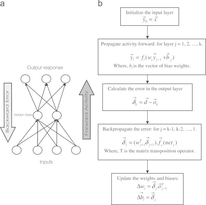
(a) A multi-layer back-propagation (BP) network with one hidden layer of units, (b) flowchart of the BP.
Fig. 2.
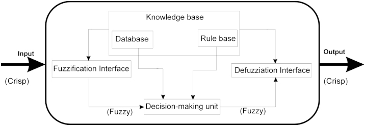
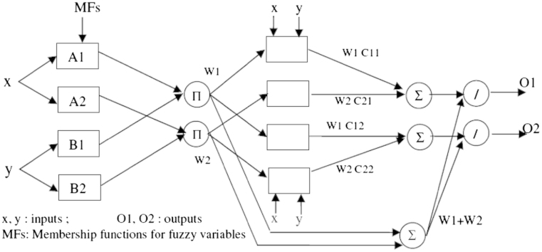
Fuzzy inference system (FIS) which is composed of five functional block: a rule base (containing a number of fuzzy if-then rules), a database (defines the MFs of the fuzzy sets used in the fuzzy rules), a decision-making unit (performs the inference operations on the rules), a fuzzification interface (to calculate fuzzy input) and a defuzzification interface (to calculate the actual output) (Jang 1993).
Jang, 1992, 1993 combined both FL and ANN to produce a powerful processing tool, named adaptive neuro-fuzzy inference system (ANFIS). ANFIS uses an ANN learning algorithm to set fuzzy rule with the appropriate MFs from input and output data. Actually, this technique is an appropriate solution for function approximation in which a hybrid learning algorithm applied for the shape and the location of MFs (Buragohain and Mahanta, 2008; Ying and Pan, 2008). Moreover, a practical example of this method is introduced in Tahmasebi and Hezarkhani (2011).
One of the main networks utilized in this study is CANFIS which belongs to a more general class of ANFIS (Jang et al., 1997). In fact, the preference of CANFIS to the other ANFIS structures is because of its ability to produce multi-output(s) by nonlinear fuzzy rules in which both ANN and FIS play a significant role to reach a better estimation (Jang et al., 1997; Mizutani and Jang, 1995). To be more clear, by combination these two techniques, ANN will help to define the FL's rules, because most of the mining and geology conditions (and specifically grade estimation) are mixed with uncontrolled ambiguities which cause the rules to be difficult to define. Hence it is considered a good idea to use the ability of ANN to train the FL. In other words, by using this new hybrid system, one can use both capabilities of FL's qualification and ANN's quantification aspects.
More detailed information of ANFIS such as their different structures and learning algorithms is also discussed in the literature (Jang et al., 1997; Kim and Kasabov, 1999).
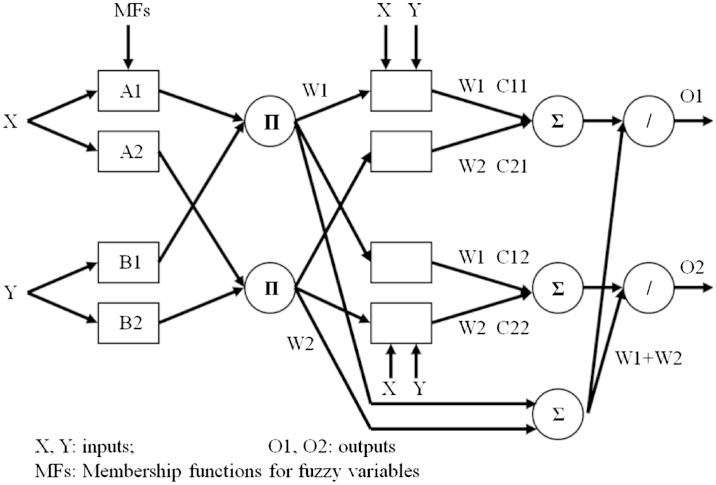
In this section, the utilized structure for the current considered case study is described. Assume that the proposed CANFIS has three inputs (x, y and z) with Cu Grade as the output (Fig. 3) and we have selected the momentum algorithm as the learning rule. The purelin transfer function has been used as the output function.
Fig. 3.
Two-output CANFIS architecture with two rules per output.
Suppose that the rules contain three fuzzy if-then rules of Takagi and Sugeno's type (Jang, 1993):
Rule 1: If x is A1, y is B1, and z is C1 then f1=p1x+q1y+t1z+ r1,
Rule 2: If x is A2, y is B2 and z is C2 then f2=p2x+q2y+t2z+ r2,
Rule 3: If x is A3, y is B3 and z is C3 then f3=p3x+q3y+t3z+ r3,
Fig. 3 illustrates the reasoning system for Sugeno model and the function of each layer is described as follows:
Layer 1 Including an adaptive node with a node function
| (1) |
where , and are any appropriate parameterized MFs and Ol,i is the membership grade of a fuzzy set A=(A1, A2, B1,B2 or C1, C2) and it indicates the degree in which the given input x (y or z) satisfied the quantifier. This layer called “Premise Parameters”.
Besides, the membership function for A can be any appropriate parameterized MF such as generalized “bell function”:
| (2) |
where {ai, bi, ci} is the parameter(s) set. As the values of these parameters change, the bell function varies accordingly and shows the various forms of MF for fuzzy set, subsequently. In the current study, this form of membership function is also used.
Layer 2 Every node in this layer is a fixed node that its output is the product of all incoming signals.
| (3) |
Each output node represents the “Firing Strength” of a rule.
Layer 3 Includes the fixed node labeled N function of normalization:
| (4) |
Simply, outputs of this layer are called “Normalized Firing Strengths”.
Layer 4 Includes the adaptive nodes:
| (5) |
Since every node in this layer is multiplication of Normalized Firing Strength from the third layer and output of ANN, hence it is called “Consequent Parameters”.
Layer 5 Includes a signal fixed node labeled Σ with function of summation which computes the overall output of CANFIS network as the summation of all the incoming signals.
| (6) |
To summarize the aim of using CANFIS, we can mention that since deciding in the parameters of the fuzzy MFs is the major difficulty in fuzzy modeling and because most of these parameters are selected by users’ experiences and/or trial and error, thus, in order to automate this process and minimize the error, a computational technique (such as ANN) can be employed. Therefore, the aim of this paper is to utilize CANFIS to construct a fuzzy inference system (FIS) which its MF's parameters are adjusted using a BP algorithm that allows the fuzzy system to capture the spatial relationships among the data and finally estimates the grade efficiently.
Considering Fig. 3, it is clear that there are still some parameters which remain non-optimal. The reason of this problem is due to using ANN. In fact, ANN tries to optimize the parameters of FL while it may trap in local minima. Although the ANN has an excellent learning algorithm and can help the FL to find the appropriate parameters, there are some parameters remaining in both ANN and FL which could have effect on performance indirectly. To encounter this problem, we use GA as a powerful optimization tool to find the best number of MFs for each input and the best values for learning rate and momentum coefficient. More details of CANFIS and GA combination are described in Sections 3.1 and 4.3.
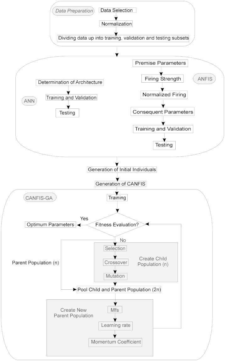
The performance of this method will be demonstrated via a case study. Besides, for the sake of comparison, we consider the performance of CANFIS–GA network, ANN and ANFIS for grade estimation. Once we obtain the results, we will evaluate the reliability of the new model by comparing the predictions with the real grade. Our methodology, CANFIS–GA, is schematically shown in Fig. 4 which is consisting of some important stages of the modeling (e.g., preprocessing, ANN, ANFIS and CANFIS–GA).
Fig. 4.
The flowchart for grade estimation and the applied methods with their designing details.
2.1. GA
The GA was first introduced by Holland (1975). It is a universal method for solving the variety of constrained and unconstrained optimization problems (Holland, 1975). GA can also be used to solve a diversity of optimization problems that are not well-suited for standard optimization algorithms, including problems in which the objective function is discontinuous, non-differentiable, stochastic, or highly nonlinear (Goldberg, 1989). Some researchers also suggested that global search techniques including the GA might prevent ANN from falling into a local minimum (McInerney and Dhawan, 1993; Sexton et al., 1998; Gupta and Sexton, 1999; Tahmasebi and Hezarkhani, 2009).
The initial population will be modified to reach a better answer. At each step, the GA selects individuals (chromosomes) from the current population (parents) randomly and uses them to produce the children for the next generation. After several generations, according to essence of the GA, it tries to move to the best solution. At each step, the GA uses three main types of rules to create the next generation from the current population. These types of rules are discussed as follows (Deb, 1999):
Selection rules select the individuals called parents which contribute to the population at the next generation.
Crossover rules combine the chromosomes in order to produce the next generation.
Mutation rules lead the chromosome to change and alter their values.
Initially, the variables should be represented by a binary string which encodes the parameters of the CANFIS and each chromosome (individuals) consists of several genes which represent the network's parameters. Then, a population of strings with initial random parameters is created as candidates of the best solution (i.e., ).
In this study, the roulette wheel method is used to determine the next chromosomes with randomly selected length. Moreover, it is possible to give a chance to the pervious chromosome to cooperate in the future generation to become a stronger chromosome. It should also be noted that in this study, we used the rulette-wheel, two-point method and boundary method for the genetic operators of selection, crossover and mutation, respectively. Afterwards, the values of fitness function (which is mainly related to the difference between the output CANFIS–GA and the real grade) are sorted and then the best and the worst chromosomes are identified (note that only the best chromosomes can crossover or mutate by rating). Therefore, the GA with the mentioned parameters is employed to obtain the optimal structure of CANFIS (e.g., Number of input neurons, membership function, learning and momentum rate).
3. Application to Sungun porphyry copper deposit in East-Azerbaijan, Northwestern Iran
3.1. Geological setting
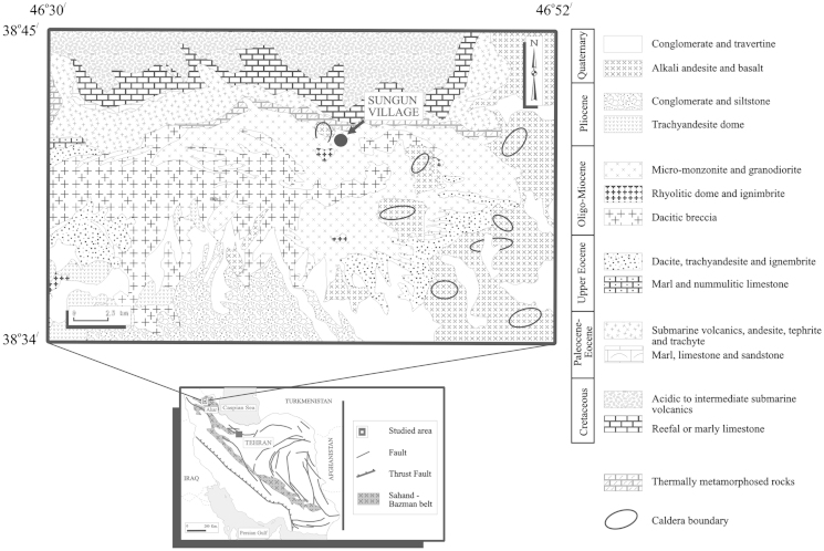
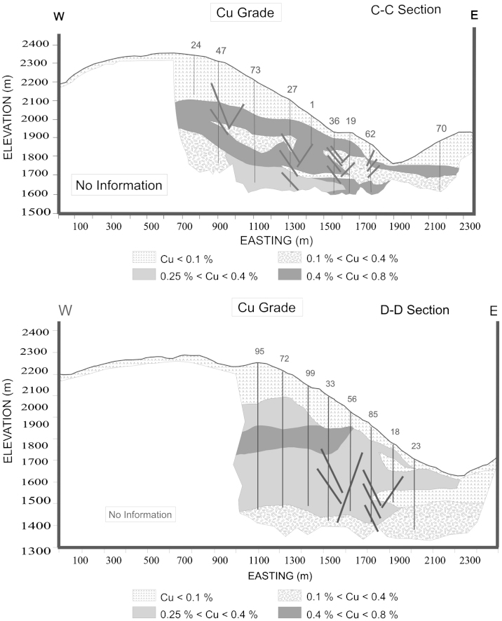
Initially, Bazin and Hübner (1969) investigated Sungun copper porphyry extensively and they reported that this reserve is a Skarn-type mineralization at the contact between the Cretaceous limestone and the granodioritic stock (Figs. 5 and 6). According to the available features and alteration indicators, Etminan (1977) supposed that this deposit is very similar to presented porphyry deposit characters by Lowell and Guilbert (1970) and he concluded that this deposit is one of the porphyry deposits (Hezarkhani et al., 1999).
Fig. 5.
Simplified geologic map of the Sungun area (Hezarkhani 2002).
Fig. 6.
Profiles showing the distribution of Cu grades along cross-sections D–D and C–C. Numbers on surface indicate drill holes (Hezarkhani 2002).
From the physico-chemical point of view, Sungun porphyry copper deposit is hosted by a composite intrusive and two main diorite/granodiorites and later a monzonite/quartz–monzonite can be seen. These reactions take place in the depth of 2000 m, and at a temperature of 670–780 °C (Hezarkhani et al., 1997). Detailed studies on fluid inclusions/isotopes, thermodynamic and reserve modelings have been provided in several studies (Hezarkhani and Williams, 1998; Hezarkhani et al., 1999; Hezarkhani, 2002).
3.2. Data preparation
At the beginning of the modeling, the data is normalized which helps to reduce the noises and finally leads to a better prediction. For this aim, different normalization methods should be tested to improve the network training (Demuth and Beale, 2002; Chaturvedi et al., 1996; Sola and Sevilla, 1997). Each of the variables are normalized by applying the following three methods to find the most effective and precise one.
These applied methods are as follows: “The original data”, “the normalized data which is in the range of [−1 1] by using the maximum and minimum dataset”, “the normalized data by using the mean and standard deviation of dataset”, and finally “the normalized data in the range of [0 1] by using the following equation”:
| (7) |
where x is the data which should be normalized, and xmax and xmin are the maximum and minimum of the original data, respectively. Moreover, Xnorm is the normalized data that is transformed. The obtained results indicate that application of final equation to normalization leads to better responses.
The applied data includes 156 exploratory boreholes. For grade estimation, the coordinates are used as input variables, and grade attribute is used as output variable for the respective dataset. In this paper, the available data for both ANN and ANFIS is divided into three and two subsets for CANFIS–GA network. For CANFIS–GA, the training and testing sets are randomly selected in the approximate ratio of 85% and 15% from the database, respectively. However, in the ordinary methods (ANN, ANFIS) which are based on trial and error, several parameters should be changed during the modeling. Therefore, the dataset needs to be validateed to control the ANN and ANFIS performance. The first subset is the training set by which the network finds an input–output spatial relationship by repetitive analysis of the training set (∼70% of whole data). The second subset is the validation set (∼15% of whole data). The difference between these two kinds of data distributions is due to applying the GA to CANFIS. While applying the GA, there is no need to come back and correct the model, because the training phase will be controlled by the GA and the best parameters are stored at each iteration. Also, we pick the sets at equally spaced points throughout the original data. Table 1 represents the summary statistics of the datasets in which the copper dataset reveals less variance.
Table 1.
Summary statistics of the using dataset.
| Data | Mean | Variance | Maximum | Minimum |
|---|---|---|---|---|
| Value | 0.379 | 0.244 | 23.5 | 0.01 |
3.3. Modeling
All the mentioned properties such as data selection, ANN's parameters, etc. were selected and considered for the modeling. It is better to explain some effective parameters in both CANFIS and GA before the modeling.
There are two fuzzy MFs: Bell-shaped and the Gaussian-shaped curves. The bell-shaped curve is a little more flexible, because it has three free parameters to adjust compared to the Gaussian-shaped MF which has only two parameters. Therefore, the bell-shaped has been selected as the employed membership function. There are also two learning updates: on-line learning, which updates the network after presenting each exemplar, and batch learning, which updates it after the presentation of the entire training set. We used the latter update in this study. Moreover, we selected the momentum and axon as the learning algorithm and the transfer function, respectively. It is important to mention that axon transfer function is the identity map which is normally used only as a storage unit, and as it is expected, its output is equal to the input. Furthermore, the momentum should be added as a composition of two main parameters. In other words, while searching with the momentum component, there are two parameters to be selected: the step size and the momentum. One solution is to set a value for the learning rates by trial and error method. As another solution, one can use the GA. Indeed, we used GA for finding the best value/number of processing elements, step size, and momentum rate. Finally, there are two variants from available CANFIS networks to choose: the Tsukamoto fuzzy model which is simple and runs fast, whereas the TSK fuzzy model (also known as the Sugeno fuzzy model) is generally more popular.
Since the chromosomes are composed of genes, the variable should be presented to GA encoded by chromosomes. As explained, there are three parameters which should be optimized; as a result, each chromosome (or a candidate of solution) is composed of three genes (learning rate, momentum of the network and the number of MFs for each input) which indicate the values of those parameters. We also used aploid chromosomes to present them to the GA. At the first step, the number of individuals will be produced randomly. Then, fitness function is evaluated for these individuals. Next, encoded chromosomes are searched to maximize the fitness function in which the quality of the solution is sorted in the fitness value and can be represented by the average prediction accuracy of the training data. In this study, we used MSE (Mean Square Error) as the fitness function which measures average of the square of error. The amount of error is interpreted by the difference between the responses of CANFIS–GA and the true (actual) grades. Eventually, the MSE is defined by the following equation:
| (8) |
where Pi is the value of predicted grade by CANFIS–GA, Tj is the real grade and n is the number of data in the training dataset. For a perfect fit, Pi=Tj and Ei=0. Thus, the MSE index range changes from zero to the infinity with zero corresponding to the ideal condition. Clearly, the MSE calculates the differences between the predicted grade by CANFIS–GA and the actual grade in the training dataset. Fig. 7 shows the best MSE for each generation in the training phase.
Fig. 7.
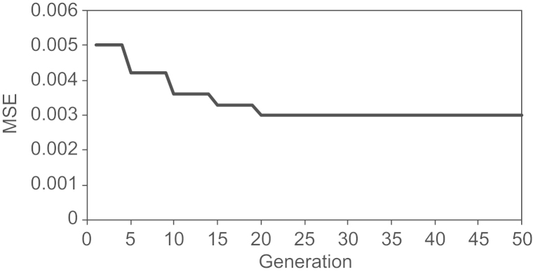
Showing the best fitness (best MSE) in the each generation that by applying GA and testing several chromosomes on each generation which each of them carrying the possible architecture or values of the parameters that should be optimized on that generation resulted.
In each successfully run of the algorithm, the fitness function is calculated according to individuals. In this section, it is possible that the calculated fitness function of individuals may not be appropriate for new generation comparing to the initial criteria; therefore, in this case the individuals are selected according to their fitness function to produce the offspring which that is indeed the result of parent recombination. Then, by using the mutation operator (which is a probability type), all the offspring will be mutated. Next, the parents will be replaced by the new offspring in order to produce a new generation. This simple cycle is the basic step in the GA because repeating this procedure and according to supposed criteria, the best answer for optimization problem would be derived. Obviously, in order to find the settings that produce the lowest error, this form of iteration-based optimization requires the network to be trained in several times.
Basically, the GA is based on the three parameters: crossover, mutation and population. The different values of these parameters are important and the GA might be sensitive to the different values. Then, the population size was set from 15 to 60 and the crossover and mutation rates may vary to prevent beginning up any possible problem and error. The range of the crossover rate was set between 0.1 and 0.9 while the mutation rate ranges from 0.01 to 0.2 and their results were compared in order to find the optimum values of different parameters. Therefore, a total of 45 experiments were performed to present the combination of the different level of mentioned parameters. Since no discrepancies were observed between the various parameters values, the middle level of each parameter was chosen as the final GA parameters (Table 2). Therefore, the GA was started with 50 randomly generated chromosomes, and their parameters were crossover rate, mutation rate and population size with the values of 0.6, 0.12 and 50, respectively.
Table 2.
Summarized results of 45 performed different experiments to present the combination of the different level of the three parameters crossover, mutation and population.
| Stage | 1 | 2 | 3 | 4 |
|---|---|---|---|---|
| Crossover rate | 0.1 | 0.3 | 0.6 | 0.9 |
| Mutation rate | 0.01 | 0.06 | 0.12 | 0.2 |
| Population size | 15 | 30 | 50 | 60 |
4. Results and discussion
4.1. Grade estimation by ANN
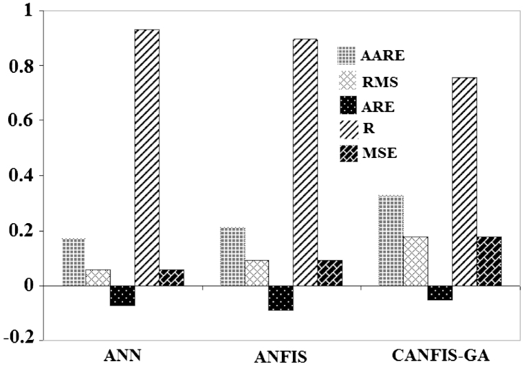
As explained earlier, the input data includes the coordination and the output is grade value. In non-optimal methods, the trial and error method is the only way to determine the optimal structure. The results for testing dataset are shown in Figs. 8 and 9. The obtained structure has the lowest MSE (Mean Square Error), RMS (Root Mean Squared), AARE (Average Absolute Relative Error), ARE (Average Relative Error) and the maximum R (correlation coefficient) (these mathematical expressions are fully defined by Rice, 2006). It is obvious that the best and desired values for all of those parameters are zero except the R value which is equal to 1. In is also noted that for more than single layer structure, the ANN was tested throughout this stage for multi-layers, but the results were not satisfying.
Fig. 8.
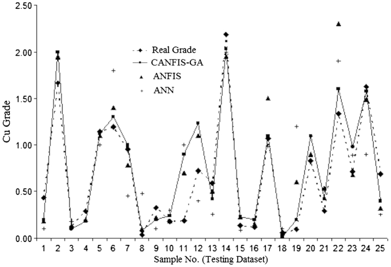
Comparison of predicted results with actual grade values for Sungun copper porphyry deposit based on the ANN, ANFIS and CANFIS–GA.
Fig. 9.
Comparison of AARE, RMSE, ARE, R, MSE for ANN, ANFIS and CANFIS–GA.
4.2. Grade estimation by ANFIS
The training of an ANFIS network which involves grade estimation, conducts the input training vectors to target vectors with a minimum total sum of squared error. All the inputs and outputs are presented to network in several iterations. As the network learns, the error drops to zero (For more information about the ANFIS training in grade estimation refer to Tahmasebi and Hezarkhani (2011)).
The training was based on 60 epochs which the hybrid learning algorithm was used in its architecture. At the end of 35 training epochs, the mean square error for validation vectors was converged to a minimum of 0.0925. Therefore, 35 epochs were selected for grade estimation process. The trained Takagi–Sugeno type fuzzy inference system was used for grade estimation of available dataset. Then, four bell-typed fuzzy MFs per each input were selected to describe the input to output variables. This is translated in 16 rules for each one regarding the two inputs with four fuzzy sets. The results of final estimator model for testing dataset are shown in Figs. 8 and 9.
4.3. Grade estimation: CANFIS–GA
According to the earlier discussion, the fitness function is “MSE” and it means that in all the network evaluations, that is considered as a rule to reach the best result. In this modeling, several networks with different crossover and mutation rates were investigated to find the best probability. As it is shown in Fig. 7, among 50 generations, the desired network with the lowest error obtained in the 20th generation. This network is the results of applying the GA to the best obtained parameter that can be used to gain the lowest error for grade estimation and the best network subsequently. On the other hand, by testing several values for the given parameters, the GA makes the network to converge to the best structure and response. These parameters are described as follows: a mutation rate of 0.08, the network with four nodes in the MFs layer, a learning rate of 0.65 and a momentum of 0.7. The optimal obtained network was presented in the 20th generation that it was located in 24th position of the 52 networks. The MSE of this optimal network in the training stage was equal to 0.003.
In order to evaluate the performance of the current methodology, 15% of the whole dataset were selected as the test dataset. The performance of CANFIS–GA gained by the test dataset is presented in Figs. 8 and 9. The predictions were then compared with the actual grade values. Fig. 8 shows the comparison of 24 grade prediction samples versus the actual grade values for CANFIS–GA. The horizontal axis represents the real grade and the vertical axis shows the obtained results from applying several techniques in this paper.
According to Figs. 8 and 9, the prediction capability of CANFIS–GA model is documented. Therefore, this network is considered to be used to predict the grade values. By applying this method, an obvious improvement on the grade estimation is obtained. The worst results were obtained from the neural network technique. The results of ANFIS are better than those of ANN due to the fact that this technique is a combination of ANN and FL methods and is better in getting the spatial relationships between the variables. The CANFIS–GA technique is expected to provide a significant improvement when the new data comes from mixed or complex distributions. Since most of the mining and geological activities can be considered to fall down in some fuzzy conditions, the CANFIS–GA could be an excellent choice compared to the other methods from the performance point of view. The proposed methodology not only has the intrinsic advantages of the neural-fuzzy techniques, but also the parameters are optimized by the GA under the new approach. Moreover, this integrated approach could improve the predictions, and in addition to geology and mining problems, this adaptive technique can be used in different fields.
5. Conclusion and future works
This paper introduces an integrated CANFIS and GA (CANFIS–GA) to predict the ore grade from the boreholes in Sungun porphyry copper deposit in Iran. It is also a simultaneous search for optimal selection to adjust the network parameters. Due to having a lot of parameters in different methods of artificial intelligence (e.g., ANN, FL and GA), these methods need a significant time and effort to find the optimal structure,. On the other hand, using this new proposed technique for grade estimation in this paper, the issues with FL such as definition of fuzzy if-then rules and number of MFs could be resolved. Furthermore, by applying the learning process, it is possible to generate a set of fuzzy if-then rules to approximate a desired grade, as shown in this paper. The ANFIS is the result of ANN and FL combination. Combining these two intelligent approaches, a good reasoning would be achieved in both quality and quantity. In other words, both fuzzy reasoning and network calculation could be available simultaneously. Since most of the related grade estimation scopes are very fuzzy and the relationship between variable is also complicated in some cases, this new methodology can be extended to be applied in most of mining and geological problems. By using the GA, it is also possible to reduce inputs in order to get the best results. In the current study the input variables were three dimensional and there was no need to reduce the variables. In cases with lots of variables, however, this method could be very helpful in input reductions. In this study, the CANFIS–GA performance was investigated extensively, whereas the correlation coefficient was equal to 0.9327 which shows that this method has an excellent performance for grade estimation. This method was compared to the other current methods, which the results indicated that the integrated neural-fuzzy and GA (GA–ANFIS) provides the least error on the testing dataset. In addition, applying the GA–CANFIS requires much less effort and also that is not very time consuming to solve the problems. Moreover, this method does not have the common problems existing in the ANN and the FL, as both the prediction accuracy and the time requirement for the solutions are improved by the proposed method.
Contributor Information
Pejman Tahmasebi, Email: pejman@aut.ac.ir.
Ardeshir Hezarkhani, Email: Ardehez@aut.ac.ir.
References
- Asadi J., Tahmasebi P. Comparative evaluation of back-propagation neural network learning algorithms and empirical correlations for prediction of oil PVT properties in Iran oilfields. Journal of Petroleum Science and Engineering. 2011 [Google Scholar]
- Bardossy A., Bogardi I., Kelly W.E. Kriging with imprecise (Fuzzy) variogram I: theory. Mathematical Geology. 1990;22(1):63–79. [Google Scholar]
- Bardossy A., Bogardi I., Kelly W.E. Kriging with imprecise (fuzzy) variograms. II application. Mathematical Geology. 1990;22(1):81–94. [Google Scholar]
- Bardossy Gy., Fodor J. Assessment of the completeness of mineral exploration by the application of fuzzy arithmetic and prior information. Acta Polytechnica Hungaricae. 2005;2(1):217–224. [Google Scholar]
- Bardossy Gy., Szabo I.R., Varga G. A new method of resource estimation for bauxite and other solid mineral deposits. Journal of Hungarian Geomatematics. 2003;1:14–26. [Google Scholar]
- Bazin, D., Hübner, H., 1969. Copper deposits in Iran , Report No 13. Ministry of Economy, Geological Survey of Iran. 365 pp.
- Buragohain M., Mahanta C. A novel approach for ANFIS modeling based on full factorial design. Applied Soft Computing archive. 2008;8:609–625. [Google Scholar]
- Chatterjee S., Bandopadhyay S., Machuca D. Ore grade prediction using a genetic algorithm and clustering based ensemble neural network model. Mathematical Geosciences. 2010;42(3):309–326. [Google Scholar]
- Chaturvedi, D.K., Satsangi, P.S., Kalra, P.K., 1996. Effect of different mappings and normalization of neural network models. Ninth National Power Systems Conference, Indian institute of Technology, Kanpur 1, pp. 377–386.
- Cheng Q., Agterberg F.P. Fuzzy weights of evidence method and its application in mineral potential mapping. Natural Resources Research. 1999;8(1):27–35. [Google Scholar]
- Clarici E., Owen D.B., Durucan S., Ravencroft P.J. Recoverable reserve estimation using a neural network. In: Elbrond J., Tang X., editors. 24th International Symposium on the Application of Computer and Operation Research in the Mineral Industries (APCOM) 1993. pp. 145–152. [Google Scholar]
- Deb K. An introduction to genetic algorithms. Sadhana. 1999;24(4–5):293–315. [Google Scholar]
- Demuth H., Beale M. Mathworks Inc; USA: 2002. Neural Network Toolbox for Use with MATLAB. [Google Scholar]
- Denby, B., Burnett, C., 1993. A neural network based tool for grade estimation, 24th International Symposium on the Application of Computer and Operation Research in the Mineral Industries (APCOM), Montreal, Quebec.
- Etminan, H., 1977. A porphyry copper–molybdenum deposit near the Sungun village. Internal Report, Geological Survey of Iran, p. 240.
- Galatakis M., Theodoridis K., Kouridou O. Lignite quality estimation using ANN and adaptive neuro-fuzzy inference systems (ANFIS) APCOM. 2002:425–431. [Google Scholar]
- Ghezelayagh H., Lee K.Y. Training neuro-fuzzy boiler identifier with genetic algorithm and error backpropagation. IEEE Power Engineering Society, Summer Meeting. 1999;2:978–982. [Google Scholar]
- Goldberg D.E. Genetic Algorithms in Search, Optimization, and Machine Learning. Addison-Wesley; 1989. 412 pp. [Google Scholar]
- Gupta J.N.D., Sexton R.S. Comparing backpropagation with a genetic algorithm for neural network training. Omega. 1999;27:679–684. [Google Scholar]
- Hezarkhani A. Specific physico-chemical conditions (360 °C) for chalcopyrite dissolution/deposition in the Sungun porphyry copper deposit, Iran. Amirkabir Journal of Sciences and Technology. 2002;13(52):668–687. [Google Scholar]
- Hezarkhani A., Williams J.A.E. Vol. 93. evidence from fluid inclusions and stable isotopes. Economic Geology; Iran: 1998. (Controls of Alteration and Mineralization in the Sungun Porphyry Copper Deposit). 651–670. [Google Scholar]
- Hezarkhani, A., Williams, J.A.E., Gammons, C., 1997. Copper solubility and deposition conditions in the potassic and phyllic alteration zones, at the Sungun porphyry copper deposit, Iran. Geological Association of Canada and Mineralogical Association of Canada (GAC–MAC), Annual Meeting, Ottawa pp. 65–72.
- Hezarkhani A., Williams J.A.E., Gammons C.H. Factors controlling copper solubility and chalcopyrite deposition in the Sungun porphyry copper deposit, Iran. Mineralium Deposita. 1999;34:770–783. [Google Scholar]
- Holland J.H. MIT Press; Cambridge: 1975. Adaptation in Natural and Artificial Systems. Ann Arbor: University of Michigan Press. (A 2nd edn was published in 1992. 183 pp. [Google Scholar]
- Hornik K., Stinchcombe M., White H. Multilayer feedforward networks are universal approximators. Neural Network. 1989;2(5):359–366. [Google Scholar]
- Ishigami H. Structure optimization of fuzzy neural network by genetic algorithm. Fuzzy Sets and System. 1995;71:257–264. [Google Scholar]
- Jagielska I., Matthews C., Whitfort T. An investigation into the application of neural networks, fuzzy logic, genetic algorithms, and rough sets to automated knowledge acquisition for classification problems. Neurocomposites. 1999;24:37–54. [Google Scholar]
- Jang, J.S.R., 1992. Neuro-fuzzy modeling: architecture, analyses and applications. Unpublished Ph.D Dissertation, Department of Electrical Engineering and Computer Science, University of California, Berkeley, California.
- Jang J.S.R. ANFIS: adaptive-network-based fuzzy inference system. IEEE Transaction on Systems, Man and Cybernetics. 1993;23(3):665–685. [Google Scholar]
- Jang J.S.R., Sun C.T., Mizutani E. Neuro-Fuzzy and Soft Computing: A Computational Approach to Learning and Machine Intelligent. Prentice-Hall International; 1997. 614 pp. [Google Scholar]
- Journel A.G., Huijbregts C. Academic Press; London: 1978. Mining Geostatistics. 600 pp. [Google Scholar]
- Kapageridis, I.K., Denby, B., 1998. Neural network modeling for ore grade spatial variability. Prpceedings of the 8th International Conference on Artificial Neural Networks (ICANN), Skovde, Sweeden, pp. 209–214.
- Kapageridis I.K., Denby B., Hunter G. Integration of a neural ore grade estimation tool in a 3D resource modeling package, neural networks. IJCNN ‘99. International Joint Conference on Neural Network. 1999;6:3908–3912. [Google Scholar]
- Ke, J., 2002. Neural network modeling of placer ore grade spatial variability. Unpublished Ph.D Dissertation, University of Alaska Fairbanks, pp. 251.
- Kim J., Kasabov N. HyFIS: adaptive neuro-fuzzy inference systems and their application to nonlinear dynamical systems. Journal of Neural Network. 1999;12:301–1319. doi: 10.1016/s0893-6080(99)00067-2. [DOI] [PubMed] [Google Scholar]
- Koike K., Matsuda S. Characterizing content distributions of impurities in a limestone mine using a feed forward neural network. Natural Resources Research. 2003;12(3):209–223. [Google Scholar]
- Koike K., Matsuda S., Gu B. Evaluation of interpolation accuracy of neural kriging with application to temperature-distribution analysis. Mathematical Geology. 2001;33(4):421–448. [Google Scholar]
- Koike K., Matsuda S., Suzuki T., Ohmi M. Neural network-based estimation of principal metal contents in the Hokuroku district, Northern Japan, for exploring Kuroko-type deposits. Natural Resources Research. 2002;11(2):135–156. [Google Scholar]
- Lacassie J.P., Solar J.R., Roser B., Hervé F. Visualization of volcanic rock geochemical data and classification with artificial neural networks. Mathematical Geology. 2006;38(6):697–710. [Google Scholar]
- Lowell J.D., Guilbert J.M. Lateral and vertical alteration– mineralization zoning in porphyry ore deposits. Economic Geology. 1970;65:373–408. [Google Scholar]
- Luo X., Dimitrakopoulos R. Data-driven fuzzy analysis in quantitative mineral resource assessment. Computers & Geosciences. 2003;29:3–13. [Google Scholar]
- Mahmoudabadi H., Izadi M., Menhaj M.B. A hybrid method for grade estimation using genetic algorithm and neural networks. Computational Geosciences. 2009;13:91–101. [Google Scholar]
- Mamdani E.H., Assilian S. An experiment in linguistic synthesis with a fuzzy logic controller. International Journal Man Machine. 1975;7(1):1–13. [Google Scholar]
- McInerney, M., Dhawan, A.P., 1993. Use of genetic algorithms with backpropagation in training of feedforward neural networks. In: Proceedings of the IEEE International Conference on Neural Networks, pp. 203–208.
- Mizutani, E., Jang, J.S.R., 1995. Coactive neural fuzzy modeling. In proceedings of the International Conference on Neural Network, pp. 760–765.
- Pham T.D. Grade estimation using fuzzy-set algorithms. Mathematical Geology. 1997;29(2):291–305. [Google Scholar]
- Porwal A., Carranza E.J.M., Hale M. A hybrid neuro-fuzzy model for mineral potential mapping. Mathematical Geology. 2004;36(7):803–826. [Google Scholar]
- Rendu, J.M., 1979. Kriging, logarithmic Kriging, and conditional expectation: comparison of theory with actual results, Proc. 16th APCOM Symposium. Tucson, Arizona, pp. 199–212.
- Rice J.A. Mathematical Statistics and Data Analysis. Duxbury Press; 2006. 85 pp. [Google Scholar]
- Ross T.J. Fuzzy logic with Engineering Applications. McGraw Hill Inc.; New York: 2006. 628 pp. [Google Scholar]
- Samanta B., Bandopadhyay S., Ganguli R. Data segmentation and genetic algorithms for sparse data division in Nome placer gold grade estimation using neural network and geostatistics. Mining Exploration Geology. 2004;11(1–4):69–76. [Google Scholar]
- Sexton R.S., Dorsey R.E., Johnson J.D. Toward global optimization of neural networks: a comparison of the genetic algorithm and backpropagation. Decision Support Systems. 1998;22(2):171–185. [Google Scholar]
- Singer D.A. Typing mineral deposits using their associated rocks and grades and tonnages in a probabilistic neural network. Mathematical Geology. 2006;38(4):465–475. [Google Scholar]
- Singer D.A., Kouda R. Application of a feed forward neural network in the search for Kuroko deposits in the Hokuroku district, Japan. Mathematical Geology. 1996;28(8):1017–1023. [Google Scholar]
- Sola J., Sevilla J. Importance of input data normalization for the application of neural networks to complex industrial problems. IEEE Transactions on Nuclear Science. 1997;44(3):1464–1468. [Google Scholar]
- Strebelle S. Conditional simulation of complex geological structures using multiple-point geostatistics. Mathematical Geology. 2002;34(1):1–22. [Google Scholar]
- Tahmasebi P., Hezarkhani A. IAMG09. Stanford University; California: 2009. (Application of Optimized Neural Network by Genetic Algorithm). [Google Scholar]
- Tahmasebi P., Hezarkhani A. Comparison of optimized neural network with fuzzy logic for ore grade estimation. Australian Journal of Basic and Applied Sciences. 2010;4(5):764–772. [Google Scholar]
- Tahmasebi P., Hezarkhani A. Application of adaptive neuro-fuzzy inference system for grade estimation; case study, sarcheshmeh porphyry copper deposit, Kerman, Iran. Australian Journal of Basic and Applied Sciences. 2010 b;4(3):408–420. [Google Scholar]
- Tahmasebi P., Hezarkhani A. Application of a modular feedforward neural network for grade estimation. Natural Resources Research. 2011;20(1):25–32. [Google Scholar]
- Tahmasebi, P., Hezarkhani, A. Multiple geostatistical simulation. In: Geostatistics, InTech Publication (in press).
- Tahmasebi, P., Hezarkhani, A., Sahimi, M. Multiple-Point Geostatistical Modeling based on the Cross-Correlation Functions, Computational Geosciences (in press).
- Takagi T., Sugeno M. Fuzzy identification of systems and its applications to modeling and control. IEEE Transactions on Systems, Man, and Cybernetics. 1985;15(1):116–132. [Google Scholar]
- Tutmez, B., 2005. Reserve estimation using fuzzy set theory. Unpublished Ph.D dissertation, Hacettepe University, Ankara, pp. 168.
- Tutmez B., Tercan E.A., Kaymak U. Fuzzy modeling for reserve estimation based on spatial variability. Mathematical Geology. 2007;39(1):87–111. [Google Scholar]
- Weller A.F., Corcoran J., Harris A.J., Ware J.A. The semi-automated classification of sedimentary organic matter in palynological preparations. Computers & Geosciences. 2005;31(10):1213–1223. [Google Scholar]
- Weller A.F., Harris A.J., Ware J.A. Two supervised neural networks for classification of sedimentary organic matter images from palynological preparations. Mathematical Geology. 2007;39(1):657–671. [Google Scholar]
- Weller A.F., Harris A.J., Ware J.A., Jarvis P.S. Determining the saliency of feature measurements obtained from images of sedimentary organic matter for use in its classification. Computers & Geosciences. 2006;32(9):1357–1367. [Google Scholar]
- Wu X., Zhou Y. Reserve estimation using neural network techniques. Computers & Geosciences. 1993;19(4):567–575. [Google Scholar]
- Yager R.R., Zadeh L.A. Fuzzy Sets Neural Networks and Soft Computing. Thomson Learning; 1994. 440 pp. [Google Scholar]
- Yama B.R., Lineberry G.T. Artificial neural network application for a predictive task in mining. Mining Engineering. 1999;51(2):59–64. [Google Scholar]
- Ying L.C., Pan M.C. Using adaptive network based fuzzy inference system to forecast regional electricity loads. Energy Conversation and Management. 2008;49:205–211. [Google Scholar]
- Zadeh L.A. Fuzzy sets. Information and Control. 1965;8:338–353. [Google Scholar]


