

Highlights
► We investigated dispatching and relocation decisions of emergency service providers. ► ADP is powerful in solving the underlying stochastic and dynamic optimization problem. ► Average response time can be improved by using more flexible dispatching rules. ► Relocating ambulances proactively improves service quality. ► Essential to take into account time-dependent information.
Keywords: OR in health services, Emergency vehicles, Ambulance location, Approximate dynamic programming, Stochastic optimization
Abstract
Emergency service providers are supposed to locate ambulances such that in case of emergency patients can be reached in a time-efficient manner. Two fundamental decisions and choices need to be made real-time. First of all immediately after a request emerges an appropriate vehicle needs to be dispatched and send to the requests’ site. After having served a request the vehicle needs to be relocated to its next waiting location. We are going to propose a model and solve the underlying optimization problem using approximate dynamic programming (ADP), an emerging and powerful tool for solving stochastic and dynamic problems typically arising in the field of operations research. Empirical tests based on real data from the city of Vienna indicate that by deviating from the classical dispatching rules the average response time can be decreased from 4.60 to 4.01 minutes, which corresponds to an improvement of 12.89%. Furthermore we are going to show that it is essential to consider time-dependent information such as travel times and changes with respect to the request volume explicitly. Ignoring the current time and its consequences thereafter during the stage of modeling and optimization leads to suboptimal decisions.
1. Introduction and related work
Emergency service providers are supposed to locate ambulances such that in case of emergency patients can be reached in a time-efficient manner. Two fundamental decisions and choices need to be made real-time. First of all immediately after a request emerges an appropriate vehicle needs to be dispatched and send to the requests’ site. Ambulances, when idle, are located at designated waiting sites. Hence after having served a request the vehicle needs to be relocated (i.e. its next waiting site has to be chosen). For a close match to reality, time-dependent information for both traveling times and the request volume will be considered explicitly. We are going to solve the underlying optimization problem using approximate dynamic programming (ADP), an emerging and powerful tool for solving stochastic and dynamic problems typically arising in the field of operations research.
In practice simple rules for dispatching and relocation are in use. In Austria, because of regulatory rules, in case of an emergency always the closest ambulance will be dispatched. After having served a request ambulances are supposed to return to their home base. Using ADP we are going to relax these assumptions and propose different strategies in order to improve the performance of the underlying system and its capability to efficiently serve emergency requests. Empirical studies suggest that after for instance a cardiac and circulatory arrest the chances for a resuscitation to be successful decrease dramatically. Typically chances decrease by 10% per minute as long as the patient is not treated accordingly. Providing a quick response to emergency requests is crucial for the patients’ state of health.
The contribution of this paper is threefold.
-
(i)
We propose a stochastic dynamic model for the ambulance relocation and dispatching problem, which will be solved by means of ADP.
-
(ii)
In order to get a preferably accurate model of reality we will explicitly take into account time-dependent information and variations with respect to changing request volumes and travel times, varying throughout the course of the day.
-
(iii)
We are able to improve dispatching and relocation strategies currently in use.
Different possibilities exist for measuring and evaluating the performance of emergency service providers. Typically timeliness is considered as the primary objective. Most performance measures are related to response or waiting times. In this paper we will try to minimize the average response time observed. We can show that it is not necessarily a good choice to always dispatch the closest vehicle available. From a global perspective it does make sense (whenever the level/priority of the request permits) to send a vehicle that might be slightly farther away. As a consequence the waiting time observed by this particular request will be marginally worse. From a global perspective however the remaining vehicles are located more effectively in order to cover future demands more efficiently. By making decisions in an anticipatory manner, while implicitly taking into account the current situation as well as potential future requests, the performance of the emergency service provider can be improved. The algorithm has been tested on real data form the city of Vienna and has been benchmarked against two myopic policies traditionally in use.
We are going to show that it is essential to consider time-dependent information such as travel times and changes with respect to the request volume explicitly. Ignoring the current time and its consequences thereafter during the stage of modeling and optimization leads to suboptimal decisions. Furthermore we have done extensive parameter testing for the proposed algorithm in use.
In the last decades several location models for the health care sector have been discussed. Typically these include the optimization of the location of ambulance vehicles, such that the population can be covered (i.e. reached) in case of an emergency effectively. Most models found in the literature are extensions of the location set covering model by Toregas et al. (1971) or the maximal covering location model by Church and ReVelle (1974). Whereas the former which tries to minimize the number of ambulances in use and the latter tries to optimize the demand covered using a fixed fleet size. These are static location problems that do not consider the fact that resources might become unavailable over time. Also the routing aspect itself is not yet present. One possibility for tackling the former concern includes multiple coverage, i.e. demand points are supposed to be covered by more than one vehicle. Such a model, called the double standard model (DSM) was introduced by Gendreau et al. (1997). Their model has been further extended with respect to capacity considerations by Doerner et al. (2005) and successfully applied to eight rural provinces in Austria. Other successful applications of models based on DSM formulations include Thirion (2006) for Belgium and Gendreau et al. (2001, 2006, 1997), who applied their models to data from Montreal.
Other possibilities for handling vehicles becoming unavailable include busy functions, where the probability that vehicles might become unavailable is modeled explicitly (see Daskin, 1983).
Several approaches already have been proposed that handle the ambulance location problem in a dynamic setting. An extension of the maximum expected coverage location problem proposed by Daskin (1983) has been developed by Repede and Bernardo (1994). Within their paper the authors propose and solve a multi-period maximum expected coverage location problems with time-variant travel times and changing fleet sizes. A similar approach, also taking into account the resulting number of relocations, has been developed by Schmid and Doerner (2010). A dynamic model for real-time ambulance relocation has been proposed in Gendreau et al. (2001), where different redeployment scenarios are precomputed. Another multi-period model for dynamic demand environment which minimized the number of ambulances required while meeting predetermined ambulance availability requirements has been proposed in Rajagopalan et al. (2008). A broad overview on different location problems and their applications in the context of ambulance location problems can be found in Brotcorne et al. (2003), Laporte et al. (2009).
We will solve the problem at hand using ADP, a very powerful approach for modeling and solving stochastic and dynamic optimization problems. Decisions (such as the choice which vehicle should be dispatched in case of a request, or where the vehicle should be sent afterwards, etc.) have to be made over time under uncertainty. Decisions that have to be made now do have an impact on the future; hence we need to find a way to anticipate their effect on future consequences (i.e. the capability of the system to serve future requests). Due to the well-known curses of dimensionality most large-scale stochastic optimization problems cannot be solved to optimality.
For a general discussion of different algorithms related to the concept of ADP we refer to Powell (2007). Similar concepts exist in other communities such as control theory (see Bertsekas and Tsitsiklis, 1996 for an overview on neuro-dynamic programming) and the computer science and artificial intelligence community (see Sutton and Barto, 1998 for an overview on reinforcement learning).
ADP has been applied successfully to resource allocation problems (see Powell et al., 2001; Godfrey and Powell, 2002a,b) and large-scale fleet management (see Simão et al., 2009; Powell and Topaloglu, 2005). For making ambulance redeployment decisions in a dynamic setting under uncertainty an ADP approach based on a policy iteration algorithm has been developed by Maxwell et al. (2009, 2010). In their papers however the authors focus on redeployment decisions (for idle vehicles) only, while maximizing the number of calls reached within a given delay threshold. In Austria however, by law, repositioning idle ambulances (apart from sending them back to a waiting location) are not allowed. Hence we try to compensate for vehicles currently being busy and the systems’ capability to cover future requests by different dispatching and relocation strategies. Furthermore, in comparison to our model, they assume travel times and call arrival rates to be constant over time.
We will give a detailed description of the model in Section 2. A mathematical formulation for the underlying dynamic and stochastic problem will be provided in Section 3. Our solution approach, which is based on ADP, will be presented in Section 4. The obtained solutions and results, as well as some additional insights and evaluations, will be provided in Section 5.
2. Problem description
Requests for emergency transportation only become known at very short notice. It is important that the system is highly flexible and robust in a sense that allows to quickly sending vehicles to the emergency site in cases needed. Hence it is crucial that idle vehicles are located and dispersed throughout the geographic area under consideration such that emergency patients can be reached quickly. The response time (i.e. the time necessary from the arrival of the call until the vehicle finally reaches the corresponding location) is a common quality characteristic for measuring the performance of ambulance dispatching services.
The dispatching process itself can be described as follows. See Fig. 1 for a graphical representation of the dispatching process.
Fig. 1.

Graphical representation of the dispatching and relocation process.
A request typically arrives by phone and is answered by a dispatcher who enters all relevant data into the dispatching system and, using a predefined set of questions, determines the priority of the call. The time at which the emergency request r becomes known to the system is denoted by tr. In case a suitable idle vehicle is available it will be assigned and it is supposed to set off towards the corresponding patient location right away (at time ar). The total dispatching time required (i.e. the time necessary from the arrival of the request until a vehicle can be assigned) is denoted by dtr. This time span typically includes the time necessary for inquiring information concerning the actual incident, identifying an adequate ambulance and typically a setup time required for the crew to get ready. Ambulances arrive (after driving for time units) at the call’s scene and start their first-aid measures at time . Service is completed (after time units) and the corresponding ambulance leaves the call’s site at . The ambulance reaches the final destination (typically a hospital) after additional units at , where the crew starts to unload the patient and she will be admit into the corresponding department. We assume that there are no setup-times required between individual events. For instance that assigned ambulances are ready to take off immediately after having been assigned. The model however could easily be extended to handle setup times for the crew to get ready before or after starting the ambulance or serving the patient. See Maxwell et al. (2010) for a detailed discussion of so called turn-out times.
The hospital where the patient is going to be hospitalized is typically not left as a choice to the dispatcher, but rather determined deterministically depending on the location of the emergency, type of incident and the availability of resources at hospitals nearby. Service is finally complete after time units at , when the vehicle is idle again and can be dispatched to a currently unassigned request r′ or relocated to a waiting location.
When idle, ambulances have to wait for future requests at designated waiting locations. In practice, as soon as an ambulance has dropped off a patient at a hospitals’ site and in case there is no further request to be served, a waiting location needs to be chosen and the ambulance will be sent there. Waiting locations might be capacity restricted in terms of the maximum number of ambulances that can wait there at any point in time. Please note that in Austria by law ambulances are not allowed to be repositioned empty from one waiting site to another one. Hence in order for the system to be prepared efficiently for serving future request, an effective redeployment strategy is indispensable.
Our overall goal is to minimize the resulting response times for all requests that occur on a given day. The underlying problem is highly dynamic and stochastic. Emergency requests are not known beforehand and typically only become known at very short notice. In case of a request the ambulance service provider needs to react immediately in order to treat the patient accordingly, provide them with first aid and take them to hospital. Two different sources of random information exist. All requests themselves are random. However time-dependent temporal and spatial distribution function of request arrivals (i.e. for their interarrival times and their corresponding location) are assumed to be available. Furthermore the duration of time during which ambulances are unavailable due to serving a request are highly stochastic. Resulting service times when picking up a patient or dropping him off are random variables themselves, for which distribution functions, which will be estimated from real-data, are assumed to be available as well. All travel times to the call’s scene , the hospital and back to the waiting site are time dependent, as speed and the resulting travel times vary throughout the day.
3. Mathematical formulation
In this section we will present a mathematical formulation for the problem at hand and the underlying dynamics. Basically two types of decisions have to be made. First of all, in case of an emergency request, the dispatcher has to decide which vehicle should be sent to the corresponding patients’ site. After having treated the patient (hopefully successfully) and dropping her off at a hospital one needs to decide where (i.e. to which waiting location) the vehicle should be sent, as vehicles cannot just stay at the hospital and wait for future requests. Requests are served based on a first-come-first-served rule. In the unlikely event that there is no ambulance available, requests will be placed in a queue and will be served at a later stage. There are two events that actually trigger a decision: upon arrival of a request and once a formerly busy vehicle is available and idle again. Hence decisions can be made at these points in time only but without loss of generality we assume that these events are frequent enough. Please note that we allow decisions to be made for any ambulance available, and not just the one triggering the event.
We will use states in order to capture the current situation of the underlying system and the dynamics involved. A systems’ state captures the status and location of all ambulances and pending requests under consideration. A detailed mathematical formulation and description of the states will be provided below.
In order to make decisions dynamically one needs to compute or (in our case) estimate the value of being in the current state, as well as the state resulting from the previous and the corresponding decision. Due to the fact decisions that are made now have a downstream impact, one needs to anticipate its effects on future consequences. More precisely in this context dispatching an ambulance in order to serve a specific emergency request has a direct impact on subsequent requests that might appear in the same region or close by.
Let St be the state of our underlying system at time t and xt the decision taken in t. The contribution (measured in terms of the resulting response times) earned for taking decision xt when in state St is denoted by C(St, xt). We could solve the problem using a myopic policy – and hence ignore the consequences of our decisions taken now – and simply solve,
| (1) |
which could be handled by means of mathematical programming quite easily. Where decision xt would be chosen, which minimizes the one-period contribution C(St, xt). As a matter of fact however decisions taken at time t do have a downstream impact and influence the state of the system in the future and the contribution earned thereafter. Dispatching and relocation decisions to be made now indirectly affect the capability to serve future emergency requests appropriately (measured in terms of the resulting response times) and the contribution earned thereafter. Any dispatching and relocation decisions made now will impact the resulting response time experienced by future requests as well, as the location of ambulances available may or may not be prepared and allow for a quick response. The underlying stochastic problem can be formulated using Bellmann’s equation in standard form
| (2) |
where is the set of all feasible states and is the one-step transition matrix indicating the probability of ending up in state s′ in the next time period t + 1 if we are currently in state St and take decision xt. The one-step transition matrix is used to compute the expectation of the value of the state we end up in t + 1. Hence this equation can be rewritten as
| (3) |
which is referred to as Bellmann’s equation in expectation form.
The underlying dynamic system evolves over time. We assume that decisions can be taken at discrete points in time only. Exogenous information (such as the arrival of new requests and their location respectively, as well as the random outcome of service times involved when serving a request) may arrive in continuous time. Thus the problem can be formulated by means of a dynamic problem.
Ambulances (Resources). At any point in time ambulances are in one of the following three statii: (i) idle (waiting) at a waiting site, (ii) currently busy with a serving or driving to a request or (iii) currently redeployed to a waiting site. Ambulances, when idle, wait at waiting locations to be dispatched to incoming emergency requests. Once an ambulance has been assigned to a request it is busy until the patient has been treated accordingly and eventually has been taken to a hospital. After serving an emergency request they become idle again and can be assigned to a new request immediately or redeployed to a waiting location.
The state of a single ambulance (i.e. our resources) in t is given by an attribute vector , where a1 and a2 specify spatial and temporal information accordingly. Depending on the status of the corresponding ambulance, when idle, a1 captures the current location, whereas a2 indicates the time since the vehicle has been waiting there. In case the vehicle is currently busy with serving a request or currently being redeployed, the attribute vector captures its destination and the expected arrival time. The set of all possible ambulance vectors a is captured by .
The state of all ambulances is modeled using the resource state vector at time t, where Rta captures the number of ambulances with attribute a in t.
Requests (Demand). Equivalently the vector of attributes for a service request is captured by b = (b1, b2, b3, b4)T, which captures its status (b1), location (b2), time it became known (b3) and priority level (b4). The status of a request might be either pending or served. Let be the set of all possible request attribute vectors b. The number of requests with attribute b in time t is denoted by Dtb. The demand state vector is given by .
The state of the entire system St in t now can be fully captured by the resource and demand state vector, i.e. St = (Rt, Dt).
Random Information. Let Wt denote the information that becomes known during interval t between t − 1 and t. The dynamics of the stochastic problem at hand can be formulated as follows. This information includes random changes in the status of our ambulances (service times might end up to be longer than originally expected) and the arrival of new emergency requests.
Dynamic Evolution. The transition functions themselves are straight forward, hence we refrain from providing a more explicit description of the transition functions involved. We can model how Rt evolves over time, which is represented using the resource and demand transition function RM and DM respectively.
| (4) |
| (5) |
The state of the system at time t is fully described by St = (Rt, Dt). Its dynamic evolution over time is modeled in terms of the state transition function
| (6) |
Decisions. The decision xt we are about to make at time t is represented using xtad, which models the number of ambulances with attribute a upon with we act on with an elementary decision of type , whereas . There exist two major decision classes for the problem at hand. First, for any given request one needs to assign available ambulances to requests. The set of ambulances currently busy is characterized by the attribute vectors , whereas (, where ) represents the attribute vectors corresponding to vehicles currently being (just becoming) idle. Let be the set of decisions to assign an ambulance to a request, where represents the decision to assign an ambulance to a request of type . Let be the set of decisions to relocate an ambulance to a waiting site.
| (7) |
| (8) |
| (9) |
| (10) |
| (11) |
Eq. (7) captures flow conservation constraints on all requests. Any request can be assigned to at most one ambulance, which is currently idle. The flow conservation constraints for ambulance are given in Eqs. (8)–(10). Only vehicles currently being idle (either at a waiting location, or just becoming idle after serving a request) can be assigned to requests. Alternatively – in case no assignment could be found – the latter group of ambulances, it has to be relocated (empty) to a waiting site. No control can be exerted on ambulances currently being busy.
Decision are made using a policy , that returns a vector of decisions xt, that are feasible in state St. The family of all decision policies is denoted by Π. The optimal policy minimizes – discounted by factor γ the expected sum of response times over the given planning horizon, using
| (12) |
4. Solution procedure
Solving the optimization problem given in (12) is usually computationally intractable. Hence we will try to tackle the problem at hand using ADP. Unlike traditional approaches based on dynamic programming, ADP is capable to handle high-dimensional state spaces and allows overcoming the curses of dimensionality typically prevalent in large scale stochastic optimization problems.
Traditionally, for a finite horizon problem and assuming there exists VT+1(ST+1) one would solve the problem at hand by means of classical (backward) dynamic programming, where one would compute the value Vt(St) from Vt+1(St+1) by stepping backward in time. This strategy however would require to evaluate Vt(St) for all . When using ADP however, we do make decisions by stepping forward in time – in an iterative fashion – by using an approximate value function. Hence instead of solving Eq. (3) we would (in iteration n) make decisions by optimizing
| (13) |
throughout a given number of iterations, where is the sample estimate of the value of currently being in state in iteration n and is the approximation obtained from from all previous iterations (up to iteration n − 1). The sample estimate obtained will then be used to update the estimate of the value function of being in state using an updating formula such as
| (14) |
where 0 ⩽ αn−1 ⩽ 1 is the corresponding step size.
As stated in Powell (2007) we encounter three curses of dimensionality. First of all the size of our state space grows very quickly, as the state vector St comes with dimension . This issue is typically addressed as the first curse of dimensionality. The second curse of dimensionality refers to the size of the outcome space for the random variable Wt, which is a vector of the same dimensions. Finally our decision vector xt is dimensioned . The problems arising from these three curses of dimensionality however can be overcome by using aggregation and a slightly different formulation of Bellmanns’ equation around the post-decision state variable, two approaches that will be described in more detail below.
Aggregation. In order to handle large state spaces we will use a concept based on aggregation in order to reduce the size of the state space. The original problem itself will be aggregated in order to compute estimates for different states and then disaggregated back in order to obtain an approximate solution for the original problem at hand. Aggregation will be used for approximating the value function only. For modeling the dynamic evolution of the system the transition functions based on the original state vector will be used. For the problem at hand we decided to use a spatial and temporal aggregation. A spatial grid will be used for the geographic area under consideration, which will be partitioned into equal (square) sub-areas. The planning horizon in terms of time is aggregated in a similar fashion. The length of the entire planning horizon (i.e. 24 hours) is split into ϕt sub-intervals. In terms of the state of the resources only the number of idle ambulances as well as the number of pending requests in the corresponding sub-areas within the corresponding time-interval will be considered. Temporal information, such as the time since those vehicles have been waiting, will be omitted. The size of the underlying spatial and temporal grid of course directly impacts the level of aggregation and the number of the resulting aggregated states. See Section 5.6.3 for a more detailed discussion on the level of aggregation involved and the resulting consequences.
Post-decision state. Due to the exogenous information process Wt, which captures the arrival of new requests and their location respectively as well as the random outcome of the observed service times, computing the expectation in Eq. (12) or (13) becomes computationally intractable. Rather than computing the expectation around the pre-decision state variable St+1, one can approximate the value function around the post-decision state variable . Let be the state at time t immediately after we made a decision (i.e. to dispatch a vehicle, relocate an ambulance or just do nothing at all), but before any new information becomes known. By using this post-decision state variable one can reformulate the transition from St to St+1 using SM,x and SM,W. SM,x captures the transition triggered by decision xt from state St to , the post decision state, which describes the state of the system immediately after making the decision but before any new information arrives. The arrival of new information Wt+1 between t and t + 1 is modeled by means of the transition function SM,W.
| (15) |
| (16) |
Similarly RM,W and RM,x (DM,W and DM,x) are used to represent the transition function of the resource (demand) state variables Rt(Dt).
Rather then estimating the value around the next pre-decision state variable St+1 we try to estimate the value for the post-decision state . From now on let be the value of being the post-decision state immediately after making a decision in t, but before any new information arises. Hence, from now on decisions would be made by optimizing
| (17) |
instead of using Eq. (13). Unlike in Eq. (14) the obtained sample estimate will then be used to update the value around the post-decision state variable using equation
| (18) |
By using forward dynamic programming in combination with the post-decision state variable we can avoid to estimate the expectation of getting into state St+1 during the stage of optimization. By approximating the value function around the post-decision state we will be able to capture the consequences of decisions taken now on the future. And most importantly the optimization problem itself reduces itself to a deterministic problem. See Ruszczyński (2010) for a more detailed discussion of post-decision states as a powerful tool in the context of ADP. There are in fact similarities between Q-learning (see Sutton and Barto, 1998) and ADP using a post-decision representation of the state variable (see Powell, 2010).
The strategy outlined before needs to initialize the estimates for the value function approximation for all states St. By default we initialize all value function approximations with 0. Computational tests however have shown that, especially during the first iterations, the performance of the policy induced by ADP starts to deteriorate and the systems’ performance is even worse than the one obtained from myopic or naïve strategies. After further iterations however the performance finally starts to improve. Myopic strategies, although their decisions are made myopically and their applicability with respect to provide good solutions on a global perspective is highly limited, tend to produce fairly acceptable solution. Hence in order to overcome this initial deterioration we decided to bias the decision process. In iteration n the decision will be made based in a purely myopic way according to Eq. (1) with probability e−δn, where δ ⩾ 0. Otherwise decisions will be made by optimizing Eq. (17). As a consequence the probability for making decisions according to the myopic rule decreases according to an exponential decay as the training phase progresses and finally approaches 0. See Section 5.6.2 for a detailed discussion of the exponential decay parameter δ, biasing the decision making process.
5. Results
In this section we are going to present the results and the performance of the tested algorithm based on ADP. The algorithm has been tested using real data, which will be presented in more detail in Section 5.1. The design of the experiments themselves, as well as the training phase of the algorithm will be described in Section 5.2. First we are going to compare the results obtained to some benchmark policies currently in use (see Section 5.3). In Austria, because of regulatory rules, in case of an emergency always the closest ambulance will be dispatched. After having served a patient and in case of any other requests to be served, the ambulance is supposed to drive back to its home base. Moving ambulances around empty is not allowed. We are going to relax two of these assumptions and show the consequences in Section 5.4. The presented algorithm will then be tested given real data (see Section 5.5). A justification for algorithmic choices such as the step size α and the level of spatial (temporal) aggregation ϕs(ϕt) will be given in Section 5.6. We finally conclude by providing additional results for potential what-if scenario for a changing fleet size and demand volume in Section 5.7.
5.1. Data
The proposed algorithm was tested using real-world data from the city of Vienna, the capital of Austria, which is located in the north-east corner of Austria. Its population amounts to a total of 1.7 million inhabitants, which corresponds to approximately 20% of Austria’s population. It extends circularly over a total area of 41.5 hectare, with a business district in the very core of the city and rather residential areas in the outskirt areas.
Real data concerning requests have been collected by Wiener Rotes Kreuz (WRK), the Viennese division of the Austrian Red Cross, during a period of two months from October to November 2009 respectively. During 42 working days (data collected on weekends and during public holidays have been omitted, because the request volume differs significantly when compared to data from working days) a total number of 3748 requests had to be answered by an ambulance, resulting in an average of 89.24 calls per day. Please note that this request volume does not reflect all emergencies in Vienna. There are several ambulance service providers, only calls having been assigned to the WRK will be taken into account. Calls themselves were generated from a spatial Poisson process. The probability distribution of interarrival times was estimated to come from an exponential distribution with parameter λt, which depends on the current time of the day t, with a global mean of 16.14 minutes, reaching its peak – in terms of the resulting request volume – between 10 am and 12 pm. See Fig. 2 for the development of λt over time.
Fig. 2.

Average interarrival time over course of day (in minutes).
The location of requests was sampled from an estimated distribution function inferred from real data. All requests are supposed to be of the same priority type and will be served on a first-come first-serve basis. See Fig. 3 for a graphical representation of the distribution of requests’ location, where darker shaded areas correspond to areas with a higher volume of emergency calls. It also shows the location of hospitals and the probability distribution for the hospital to be chosen, which was also inferred from historical data. The higher the number of patients that have been hospitalized the larger the corresponding symbol. In practice in the city of Vienna the choice of hospital is not left as a decision to the dispatcher, but is rather determined deterministically due to several attributes such as the location and type of the emergency request, the availability of resources at the hospitals and contractual allocation strategies.
Fig. 3.

Distribution of requests and hospitals.
The probability distribution for the time necessary for serving a patient at the call’s (hospital’s) site was inferred from historical data and was estimated to come from a gamma distribution with parameters θ = 3.57 and k = 6.2 (θ = 5.02 and k = 3), with an average of 22.12 (15.05) minutes respectively. The ambulance service provider currently operates 14 ambulance vehicles which can be located at 16 different waiting locations. A real-world road network from Teleatlas using all streets accessible by car has been used. The location of hospitals and patients have been geocoded using their address and have been mapped to the closest junction on the network. Floating car data was used in order to estimate time dependent variations in travel time on each link over the course of time. See Fig. 4 for a graphical representation of the road network and the location of waiting sites. Due to capacity restrictions prevailing at waiting sites at most two ambulances can be located there at any point in time. This is due to limited space for accommodating both vehicles and staff members.
Fig. 4.

Road network and waiting locations.
5.2. Experiment setup
In order to test the performance of the algorithm based on ADP the following experiment was conducted. Within a first training phase the algorithm was run for 105 iterations, where any iteration n corresponds to one single day. Random information (such as the arrival of new requests, their timing and location respectively as well as duration of service times) were sampled from the corresponding estimated distribution functions. The step size α was set to 0.2. The exponential decay parameter δ was set to 0.001. The discounting factor γ has been set to 1. The approximated value functions were initialized to 0 for all states St. The spatial and temporal aggregation parameters ϕs and ϕt were set to 4 respectively. The initial location of ambulances was determined by solving a static ambulance location problem (taking into account average travel times) metaheuristically by means of Variable Neighborhood Search (see Schmid and Doerner, 2010 for more details).
In order to show the potential when deviating from traditional dispatching and relocation rules – and the consequences in terms of the resulting situation – we have chosen a two-step procedure. First we are going to evaluate the effects of different relocation rules. Currently vehicles once empty and idle again are sent back to their home location. For our algorithm based on ADP however we are going to relax this assumption. Section 5.3 provides an overview on the results obtained. Next we will relax the dispatching rule in addition and also consider other vehicles (such as the second or more closest idle vehicle) for dispatching. The results obtained can be found in Section 5.4. We can show that relaxing both assumptions dramatically allows to improve the performance of the underlying system.
Upon completion of the training phase in the subsequent testing phase the obtained estimates for the value functions were applied. The location and timing of requests were taken from real data (rather than sampled from a distribution) and fed into the algorithm and the performance of the algorithm was evaluated accordingly. The results obtained are reported in Section 5.5.
5.3. Comparison with baseline and random policies
Dispatching is typically done by hand by experienced dispatchers. They have access to a graphical user interface that indicates the position and status of all ambulances available. Requests are supposed to be served on a first-come-first-served basis. Due to regulatory rules, in case of an emergency, always the closest ambulance available will be dispatched. For now also for the ADP we stick to this convention and focus on the relocation strategy only. We compare the performance of our ADP algorithm to three myopic policies. The question at hand now is, in case there is no further request that could be served immediately afterwards, where (i.e. to which waiting location) the ambulance should be sent in order to wait for subsequent requests. According to a highly naïve strategy one could relocate the ambulance to the closest feasible waiting location once it has finished serving a request. According to the policy currently applied at the emergency service provider, ambulances are supposed to return to their home location. Furthermore – just for comparison reason – we have also implemented a random strategy, where the next waiting location for idle vehicles will be determined randomly. The results obtained are depicted in Fig. 5, where we show the outcome when sampling 105 days. If not stated otherwise the presented results are average response times observed within the previous min{n, 4000} iterations. Due to the random component of the underlying algorithm the results have been averaged over five independent test runs. According to the current policy (dashed line in black) the average response time observed is 4.60 minutes. Following the naïve strategy (dashed line in grey) the resulting average response time amounts to 4.61 minutes. That is to say that the impact of relocating vehicles to the closest waiting location (capable of accepting the ambulance in terms of capacity considerations) around vs. sending them back to their home location is negligible. When selecting the waiting locations randomly (dotted line) the resulting average response time amounts to 5.12 minutes. These variations are due to two facts. First when selecting the next waiting location in a poor way, the systems capability to serve future requests is badly impacted. Secondly, when selecting waiting locations that tend to be far away, ambulances spend a comparatively high fraction of their driving around empty, while they cannot be dispatched to any incoming requests. Please note that we assume that only vehicles currently idle and standing still are available for dispatching. According the policy induced by our ADP algorithm (solid black line) the resulting average response time however can be decreased to 4.05 minutes, which corresponds to a decrease of 12.08% on average with respect to the current policy in use. When taking into account the state of the system (i.e. the situation from the waiting locations’ point of view and the number of ambulances currently located there, as well as time dependent fluctuations in demand, travel time and the resulting changes in coverage) one can improve the systems performance dramatically.
Fig. 5.

Average response time (in minutes) when dispatching closest vehicle.
Run times however are not an issue. During training phase it took on average 0.015 seconds per iteration to train the algorithm based on ADP. The algorithms were implemented in C++. All experiments were conducted on a computer using a Pentium D processor with 3.2 GHz.
5.4. Always dispatch closest vehicle?
Due to regulatory reasons always the closest vehicle is dispatched. For various reasons in case of urgent and life-threatening calls the closest vehicle should be sent to the patient. For requests that are not life-threatening by nature however one should definitely take into consideration to go off this rule, as the resulting global solution obtained can be improved considerably. The second or more closest idle vehicle may also be sent without compromising the patients’ safety and medical situation. Sending another than the closest idle vehicle obviously leads to a deterioration of the response time observed by the current patient under consideration. It allows however to improve the situation for potential future calls. In order to evaluate the consequences of the choice of vehicle that should be dispatched we have also allowed our ADP algorithm to learn which ambulance should be sent to the emergency’s site, rather than just sending the closest one available. The new results obtained are shown by the thick solid lines in Fig. 6. By allowing any idle ambulance to be dispatched, obviously the response time experienced by an individual request could deteriorate. On a global perspective however the average response time decreases from 4.05 (σ = 0.34) to 4.01 (σ = 0.33) minutes.1 This corresponds to a decrease of 12.89% on average with respect to the current policy in use.
Fig. 6.

Average response time (in minutes) when allowing to dispatch any vehicle.
Especially in the first stage of the training phase (n < 5000), the performance obtained using a more flexible dispatching rule is worse. This is due to the fact the algorithm needs additional training effort when deviating from the traditional dispatching strategy. Afterwards however (5000 < n < 20000) the learning process speeds up and in the long run better results can be obtained by deviating from the traditional dispatching rule and allowing any vehicle to be dispatched.
5.5. Results on real-data
After training the ADP algorithm the policy (i.e. the approximated value functions) will be applied to real data. Again the results obtained by our ADP algorithm (as described in Section 5.4, relaxing both assumptions concerning dispatching and relocations) are benchmarked against two policies (current, random). Table 1 shows the average response times obtained for these policies under consideration. The presented values are averages obtained for all 42 instances, coming from five independent test runs. The best results are highlighted in bold. The average response time observed when applying ADP amounts to 4.04 minutes, compared to 4.35 minutes when applying the current dispatching policy, which corresponds to an improvement of 7%. Please note that these figures slightly deviate from the numbers reported in Sections 5.3 and 5.4. The difference however is statistically insignificant.2 This shows once more that it is crucial to deviate from standard dispatching and relocation rules. By introducing more flexibility and the guidance of ADP when it comes to make dispatching and relocation decision one can dramatically improve the systems’ performance. This is due to the fact that decisions are made in a proactive fashion, taking into account the downstream impact on future emergency calls.
Table 1.
Comparison of different policies on real data w.r.t resulting response time.
| Policy | Response time (in min) |
|||
|---|---|---|---|---|
| Average | Minimum | Maximum | σ | |
| current | 4.35 | 3.73 | 5.21 | 0.52 |
| random | 5.04 | 4.44 | 5.65 | 0.32 |
| adp | 4.04 | 3.07 | 5.02 | 0.42 |
Fig. 7 shows a more detailed representation of the situation during the course of the day. Due to time-dependent variations in travel times and the request volume in term of incoming calls, the resulting response times vary dramatically. The performance of the ADP algorithm and the policy currently in use are comparable during peak hours. It can be seen easily however that especially during non-peak hours the proposed method improves the solution obtained. The resulting average response times considered on an hourly basis can be decreased by up to 0.7 minutes.
Fig. 7.

Average response time (in minutes) for real data (testing phase).
5.6. Discussion of algorithmic choices
In order to justify the algorithmic choices we have executed additional test runs to support the parameter settings, such as the step size and the level of aggregation chosen.
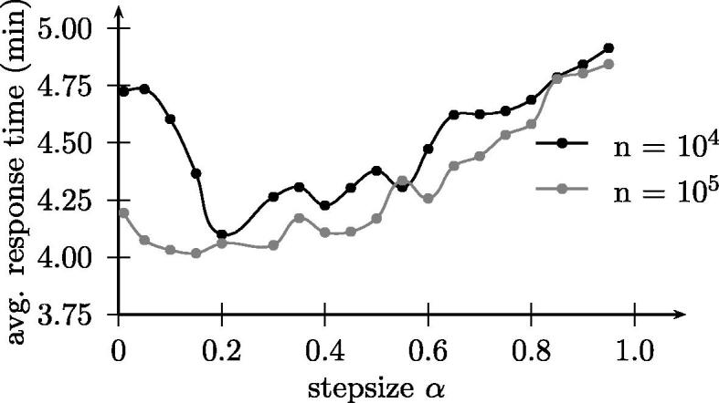
5.6.1. Stepsize
The stepsize α is basically a smoothing parameter used for updating the approximation of the value functions accordingly using Eq. (18). We decided to use a constant step size α. After extensive computational testing setting α to 0.2 has been found to be a reasonable choice. The stepsize has been varied between 0.01 and 0.95. The results obtained when using various step sizes are depicted in Fig. 8. The presented results are average response times obtained within the last 103 iterations after 104 and 105 iterations respectively. The results have been averaged over five independent test runs. Choosing a step size α which is too high impacts the (rate of) convergence. If set inappropriately the algorithm might not converge at all. After 104 iterations the choice of α still has an impact on the quality of the solution obtained. After 105 iterations however the algorithm provides more or less stable results for values of alpha set between 0.01 and 0.5.
Fig. 8.
Solution quality depending on step size α.
Please note that the step size has a significant influence on the rate of the convergence of the algorithm and the solutions produced thereafter. Alternatively one could also consider taking into account deterministic step sizes that decrease as the search process progresses or stochastic rules, where the step size would also depend on the history of the search process itself. We are planning to investigate the choice of step size in more detail in the future.
5.6.2. Policy’s exponential decay parameter
As stated in Section 4 there are different ways how decisions can be made dynamically. Our ADP algorithm needs some training before it is capable of providing satisfying results. We observed that during the first iterations the strategy proposed by ADP performs even worse than the one obtained from the current strategy. Hence we decided to bias the decision process itself. Rather than relying on the value function approximations only, decisions will also be made by applying the policy which is currently applied by our manual dispatchers (i.e. dispatch the closest vehicle and redeploy them to their home base once available again). This allows improving the learning progress. The probability for applying the current dispatching strategy is exponentially decreasing as the training phase progresses and will be applied with probability e−δn, where δ ⩾ 0 and n denotes the current iteration counter.
Fig. 9 shows the results obtained when varying the level of δ. The higher the value of δ the lower the probability that decisions will be taken according to the strategy currently in use. The probability decreases exponentially as the training phase progresses, but still proportionally less weight will be put on the current strategy during the first phase. If δ is set to 0 the underlying policy resembles the strategy currently in use.
Fig. 9.

Solution Quality depending on ADP policy’s exponential decay parameter δ.
5.6.3. Effect of level of aggregation
As outlined in Section 4 the state space is going to be aggregated accordingly. Value function approximations are estimated for states on an aggregated level only. This is done by means of both a spatial and temporal aggregation. Please note that aggregation will be used for estimating the value function only. For modeling the dynamic evolution of the system states will be considered at its original level of detail. The geographic area under consideration will be partitioned into quadratic sub-areas of equal size. Empirical tests have shown that the algorithm based on ADP performs best at a level of ϕs = 4. Temporal aggregation is done in a similar fashion, where the planning horizon is split into ϕt subintervals of equal length. Computational pre-tests indicate that setting ϕt to 4 provides the best results.
More details on the consequences concerning the choice of these aggregation parameters can be found in Figs. 10a and 10b respectively. The presented results are average response times observed after 104 training iterations.
Fig. 10a.

Average response time depending on chosen level of temporal aggregation ϕt.
Fig. 10b.
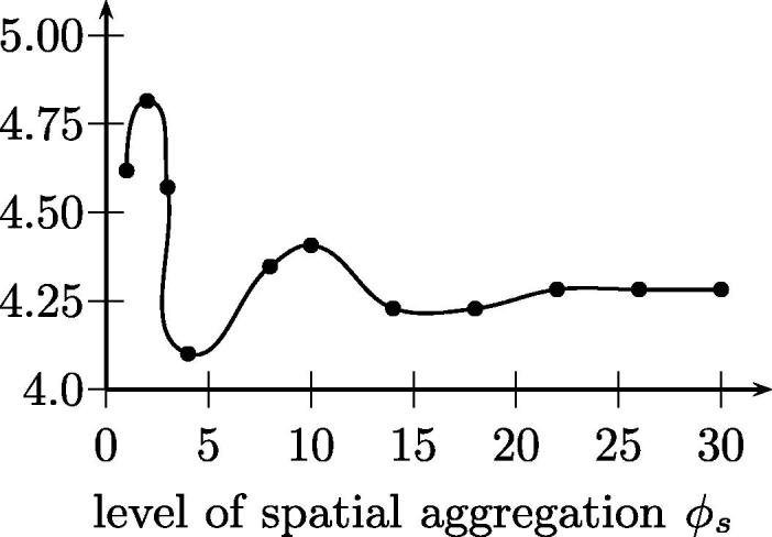
Average response time depending on chosen level of spatial aggregation ϕs.
5.7. Potential scenarios
In order to test the proposed algorithm and check the feasibility of the underlying model we conducted several additional experiments for several what-if scenarios. In particular we altered the request volume and the fleet size (i.e. the number of ambulances available).
In the investigated time period on average 89 calls requiring emergency assistance were received per day. In order to evaluate the systems behavior under a varying request volume, we altered – ceteris paribus – the average number of calls per day between 50 and 300. Any change in the call volume was assumed to have a homogeneous impact on the corresponding time-dependent rates (i.e. a x% increase with respect to the average number of calls per day was supposed to augment all underlying time-dependent rates by x% as well). A slight increase in the request volume to 100 results in an increase of the observed average response time of 0.6%. An increase to 200 (300) requests per day would – given the current infrastructure and resources – involve an increase of the observed average response time of 20.0% and 285.4% respectively.
With respect to the fleet size in use the following marginal contributions could be observed. The marginal effect of adding two more vehicles to the fleet of 14 vehicles currently in use results in a decrease of the average response time observed of 8.99%. If the fleet size is decreased by two ambulances the average response time increases by 2.23% accordingly. Once there are only 8 or less ambulances available the average response reaches a level of 6 minutes or higher.
See Figs. 11a and 11b for additional details.
Fig. 11a.

Average response time depending on number of requests per day.
Fig. 11b.

Average response time depending on available fleet size.
6. Conclusion and outlook
In this paper we formulate a dynamic version of the ambulance dispatching and relocation problem, which has been solved using ADP. Extensive testing and comparison with real-world data have shown that ADP can provide high-quality solutions and is able to outperform policies that are currently in use in practice. The average response time can be decreased by 12.89%. This improvement is due to two main sources for improvement: the dispatching and relocation decisions involved. By deviating from the traditional rule of dispatching the closest ambulance available and relocating them to their home base after having finished serving a request we are able to make high-quality dispatching decisions in an anticipatory manner. By explicitly taking into account the current state of the system we are able to improve the performance thereafter. Due to regulatory reasons ambulances are not allowed to travel around empty and to be relocated from one waiting location to another one in order to response to potentially undercovered areas. But we are able to compensate for that by locating ambulances after becoming available again in a reasonable way.
In the future we are planning to include more realistic features, such as different call priorities, more flexible and realistic dispatching rules into our model. Different priority levels shall be considered explicitly with different dispatching rules depending on the severity of the emergency. Furthermore so far we assumed only ambulances currently idle and standing still are available for dispatching. We would like to relax this assumption and also consider ambulances currently being relocated. By law ambulances are not allowed to be repositioned from one waiting site to another one. Hence in our model up to now only vehicles just becoming available after having served a patient were eligible for being relocated. We are planning to relax this assumption and allow all idle vehicles located at (or currently on their way to) a waiting site to be relocated to a (different) waiting location.
For the algorithm based on ADP we are planning to test other solution approaches based on bases functions and gradient methods, besides the pure aggregation approach we have currently chosen.
Acknowledgements
Financial support from FWF Translational Research, project number #L510-N13, is gratefully acknowledged. Special thanks go to Michel Gendreau and Karl F. Doerner for proposing this interesting field research and their support respectively.
Footnotes
According to the independent t-test for unequal variances the difference is significant for t(39972) = −11.097, p < 0.001.
The average response times observed by our version of ADP for real data are slightly worse (4.04 vs. 4.01). This difference however is not significant according to an independent t-test for unequal variances, t(211) = −1.070, p > 0.10.
References
- Bertsekas D.P., Tsitsiklis J.N. Athena Scientific; 1996. Neuro-Dynamic Programming. [Google Scholar]
- Brotcorne L., Laporte G., Semet F. Ambulance location and relocation models. European Journal of Operational Research. 2003;147(3):451–463. [Google Scholar]
- Church R., ReVelle C. The maximal covering location problem. Papers in Regional Science. 1974;32(1):101–118. [Google Scholar]
- Daskin M.S. A maximum expected covering location model: Formulation, properties and heuristic solution. Transportation Science. 1983;17(1):48–70. [Google Scholar]
- Doerner K.F., Gutjahr W.J., Hartl R.F., Karall M., Reimann M. Heuristic solution of an extended double-coverage ambulance location problem for Austria. Central European Journal of Operations Research. 2005;13(4):325–340. [Google Scholar]
- Gendreau M., Laporte G., Semet F. Solving an ambulance location model by tabu search. Location Science. 1997;5(2):75–88. [Google Scholar]
- Gendreau M., Laporte G., Semet F. A dynamic model and parallel tabu search heuristic for real-time ambulance relocation. Parallel Computing. 2001;27(12):1641–1653. [Google Scholar]
- Gendreau M., Laporte G., Semet F. The maximal expected coverage relocation problem for emergency vehicles. Journal of the Operational Research Society. 2006;57:22–28. [Google Scholar]
- Godfrey G.A., Powell W.B. An adaptive dynamic programming algorithm for dynamic fleet management, I: Single period travel times. Transportation Science. 2002;36:21–39. [Google Scholar]
- Godfrey G.A., Powell W.B. An adaptive dynamic programming algorithm for dynamic fleet management, II: Multiperiod travel times. Transportation Science. 2002;36:40–54. [Google Scholar]
- Laporte G., Louveaux F.V., Semet F., Thirion A. Innovations in Distribution Logistics. Springer; 2009. Applications of the double standard model for ambulance location; pp. 235–249. (Lecture Notes in Economics and Mathematical Systems). [Google Scholar]
- Maxwell, M.S., Henderson, S.G., Topaloglu, H., 2009. Ambulance redeployment: An approximate dynamic programming approach. In: Rossetti, M.D., Hill, R.R., Johansson, B., Dunkin, A., Ingalls, R.G. (Ed.), Proceedings of the 2009 Winter Simulation Conference.
- Maxwell M.S., Restrepo M., Henderson S.G., Topaloglu H. Approximate dynamic programming for ambulance redeployment. INFORMS Journal on Computing. 2010;22(2):266–281. [Google Scholar]
- Powell W.B. Wiley-Interscience; 2007. Approximate Dynamic Programming: Solving the Curses of Dimensionality. [Google Scholar]
- Powell W.B. Merging AI and OR to solve high-dimensional stochastic optimization problems using approximate dynamic programming. INFORMS Journal on Computing. 2010;22(1):2–17. [Google Scholar]
- Powell W.B., Topaloglu H. Applications of Stochastic Programming. Math Programming Society; 2005. Fleet management; pp. 185–215. (SIAM Series in Optimization). [Google Scholar]
- Powell W.B., Shapiro J.A., Simao H.P. A representational paradigm for dynamic resource transformation problems. Annals of Operations Research. 2001;104:231–279. [Google Scholar]
- Rajagopalan H.K., Saydam C., Xiao J. A multiperiod set covering location model for dynamic redeployment of ambulances. Computers and Operations Research. 2008;35(3):814–826. [Google Scholar]
- Repede J.F., Bernardo J.J. Developing and validating a decision support system for location emergency medical vehicles in louisville, kentucky. European Journal of Operational Research. 1994;75(3):567–581. [Google Scholar]
- Ruszczyński A. Post-decision states and separable approximations are powerful tools of approximate dynamic programming. INFORMS Journal on Computing. 2010;22(1):20–22. [Google Scholar]
- Schmid V., Doerner K.F. Ambulance location and relocation problems with time-dependent travel times. European Journal Of Operational Research. 2010;207(3):1293–1303. doi: 10.1016/j.ejor.2010.06.033. [DOI] [PMC free article] [PubMed] [Google Scholar]
- Simão H.P., Day J., George A.P., Gifford T., Nienow J., Powell W.B. An approximate dynamic programming algorithm for large-scale fleet management: A case application. Transportation Science. 2009;43(2):178–197. [Google Scholar]
- Sutton R.S., Barto A.G. MIT Press; 1998. Reinforcement Learning: An Introduction. [Google Scholar]
- Thirion, A., 2006. ModFles de localisation et de rTallocation d’ambulances: Application aux communes en provinces de Namur et Brabant Wallon. Ph.D. thesis, FacultTs Universitaires Notre-Dame de la Paix, Namur, Belgium.
- Toregas C., Swain R., ReVelle C., Bergman L. The location of emergency service facilities. Operations Research. 1971;19(6):1363–1373. [Google Scholar]