FlexE: Using elastic network models to compare models of protein structure

Abstract

It is often valuable to compare protein structures to determine how similar they are. Structure comparison methods such as RMSD and GDT-TS are based solely on fixed geometry and do not take into account the intrinsic flexibility or energy landscape of the protein. We propose a method, which we call FlexE, that is based on a simple elastic network model and uses the deformation energy as measure of the similarity between two structures. FlexE can distinguish biologically relevant conformational changes from random changes, while existing geometry-based methods cannot. Additionally, FlexE incorporates the concept of thermal energy, which provides a rational way to determine when two models are “the same”. FlexE provides a unique measure of the similarity between protein structures that is complementary to existing methods.

1 How can we measure the similarity between two protein structures?

Often, there is a need to compare two protein structures. Comparisons are commonly made on a geometric basis, such as the root mean square deviation (RMSD) of the Cartesian coordinates of the best superposition of the two structures. But there are some problems with this. First, RMSD is not independent of the protein size¹. Second, if the differences in structure are localized to a particular region, a superposition using a single alignment will lead to a spurious distribution of differences more globally throughout the structures. RMSD is not able to distinguish between a large change localized to a small region of the protein and a smaller change distributed globally across the entire structure. Given the importance of this problem, a large effort has been undertaken to improve on these metrics ranging from the use of Gaussian-weighted RMSD², to introducing a rough approximation to protein flexibility^3–6. One such alternative is to use local-global alignments (LGA)⁷. Here, many superpositions are performed and the score is given as the maximum fraction of Cα atoms that are positioned correctly to within a certain cutoff. This measure is size-independent and the choice of cutoff specifies the resolution of the structural comparison. The global distance test total score (GDT-TS) is a commonly used metric of structural similarity that measures the average fraction of residues that are correct with 1, 2, 4, and 8Å cutoffs. GDT-TS is based on four different superpositions at different resolutions and is better able to distinguish between local and global changes than RMSD. GDT-TS has become the de facto standard for measuring structural similarity in the Critical Assessment of Structure Prediction (CASP) series of experiments⁸, although several other scores, including RMSD, are also used. For the purpose of this communication we will refer to geometric scores in general to mean either RMSD or GDT-TS.

There is an additional limitation of geometric structure comparisons. When comparing theoretical models, it is more relevant to compare energies than structures, because energy is the currency for understanding thermodynamically stable states and Boltzmann populations. Moreover, energies are the basis for protein motions and function^9–13. Because energy surfaces are not isotropic, proteins can deform easily along some directions (flexible directions or soft modes) and deform very little in other directions. Thus, two different deformations of a protein that have exactly the same RMSD can potentially have very different energies (see Figure 1).

Figure 1.

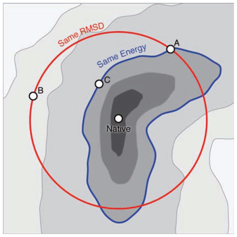
Schematic representation of conformational space showing the RMSD and energy for three structures. Structures A and B have the same RMSD, but Structure A has a lower energy. Structures A and C have the same energy, but Structure A has a higher RMSD.

Here, we describe an energy-based method for comparing two protein structures. On the one hand, the only way this could be done without error would be if we knew the exact potential function and fully simulated the free energy differences between the two conformations, for example by molecular dynamics¹⁴. But such simulations would be prohibitively expensive. Furthermore, despite their atomistic nature, the current physical models governing simulations, despite their successes, are still too coarse to fully agree with all experimental data. Normal mode analysis¹⁵ (NMA) based on these atomistic potentials is faster, but still requires hours of computational time.

In the absence of a perfect energy function, and with the aim of a fast approximate computational methodology, here we use Elastic Network Models (ENM)^16–20. This allows us to capture protein energies, motions and flexibility with small computational cost (seconds on a desktop) while still giving a relatively good correlation with more expensive MD and NMA methods^21;22. ENM is often used to calculate normal modes (NMs) describing the collective modes of motion of the system. Our approach is different and novel: rather than calculating NMs, our interest is in obtaining an ENM based Hamiltonian around a reference structure, call it A. We then use this Hamiltonian to calculate the deformation energies (FlexE score) needed to sample a different conformation, B. In this way, we compare the energies of structures A and B. This is especially useful when the reference structure is a native structure and we want to evaluate the quality of theoretical models, such as in CASP comparisons. FlexE allows us also to relate energy differences between A and B to the thermal energy, $\frac{3}{2}N{k}_{B}T$ of a system, where k_B is Boltzmann’s constant, T is the absolute temperature, and N is the number of residues. This allows us to say when two structures are within the thermal ensemble envelope around a native structure.

FlexE has some advantageous aspects: (1) independence from superposition criteria, (2) protein topology and flexibility are taken into account, (3) it can be used alone or with other metrics to assess protein model quality, (4) differences can be expressed on a per-residue basis, so it is independent of protein size. In this work we will show the application of FlexE on two datasets: (1) structures involving large conformational transitions where the end states have been experimentally determined²³; (2) the predictions from the refinement portion of the most recent CASP event (CASP9)²⁴. We show that FlexE gives energies comparable to thermal energies for all pairs of structures in the first group. Furthermore, we find that FlexE can distinguish these biologically relevant motions from motions that have similar magnitude but are generated randomly. RMSD and GDT-TS cannot make such distinctions.

2 Methods

2.1 ENM

In elastic network models, proteins are modeled as beads (one per residue). Taking one structure as reference, the distribution of these beads in space systematically defines a set of pairwise springs (between beads located within an interaction cutoff distance), all of which are at their equilibrium lengths. Any conformation different than the reference will stretch those springs and the energetic cost of deforming the spring can be obtained according to Equation 1. The collection of all springs defines the Hamiltonian of the system and the total cost of deforming the structure is the addition of the energies for all springs.

$$V_{ij}=(1/2)\gamma {(d_{ij}-d_{ij}^0)}^2$$ (1)

Where γ is the spring force constant and d_ij represents the distance between two beads, where the superscript 0 is used to indicate the distance in the reference structure. The novel use of ENM resides in using directly this Hamiltonian to evaluate structures instead of deriving a Hessian to obtain the normal modes. There are several different elastic network models in the literature which differ in the choice of which springs to use and how to assign force constants. In the initial Rouse polymer model, springs were attached to beads (for proteins usually the Cα) that were contiguous in sequence space²⁵. In the application to proteins, distance cutoffs were additionally introduced to take into account non-bonded interactions in proteins (thus taking into account the topology of the protein). Although these models capture the correct directions and relative magnitudes of motion, the absolute amount of motion along each deformation mode must be matched a posteriori to experiment (typically by matching X-ray crystallographic B-factors). This is due to the choice of spring constants when building the Hamiltonians. Several implementations introduce parameter free ENMs, where the spring constants are typically replaced by distance dependent generic functions that reproduce some underlying physical argument (such as reproducing experimental B-factors or MD trajectory data)^26–29. Recently, Orozco and coworkers¹⁹ introduced another parameter free ENM to better correlate with MD data (ED-ENM) and make it independent of scaling factors. In order to do this, two kind of springs are used. Residues close in sequence (from residue i up to i+3) follow one derivation. Residues that are close in space and not included in the first group have a different derivation (for details see¹⁹). We have used his functional form with a 12 Å cutoff in the current work since it gives us an absolute energetic scale and allows us to compare to the thermal energy of the system. In cases where only relative energies, rather than absolute energies, are important (e.g. comparing structures within an ensemble), any other ENM methods would be equally suitable^16;18;30;31.

The steps involved in creating the ENM can be schematically viewed in Figure 2. Implementation was carried out by using the existing Prody package³² from the Bahar lab and adding a small Python add-in to include the new ED-ENM method (available http://github.com/laufercenter/FlexE).

Figure 2.

Creation of an elastic network model. First, the model is reduced to just the Cα atoms. Next, springs are added for contacts that are close in sequence (up to i+3). Finally, springs are added for atoms that are close in space with a force constant that varies with distance. The strength of each spring is indicated by the thickness of each line.

2.2 Molecular Dynamics Simulations

Simulations were performed for the dataset of structures from CASP9 that: (1) did not have broken chains due to missing residues and (2) were monomers. Short 12 ns MD trajectories were performed using the AMBER³³ program package with the parm99SB forcefield in explicit TIP3P³⁴ water. Proteins were neutralized using Cl⁻ or Na⁺ ions as needed^35;36. The particle mesh Ewald method^37;38 was used for electrostatic interactions and a 2 fs time step with SHAKE³⁹ on hydrogen bonds was used. Temperature was maintained by using Langevin dynamics and a weak coupling algorithm was used to maintain pressure. We took 200 structures from the last 1ns of simulation (5 picosecond spacing) to constitute the thermal ensemble and represent conformations that are easily accessible on the energy landscape of the protein.

2.3 FlexE

The energetic cost of deforming one structure into another is defined as:

$$\mathit{FlexE}=\frac{1}{N}\sum _i^{n}0.5k_{ij}{(d_{ij}-d_{ij}^0)}^2$$ (2)

Where n is the number of inter-residue distances below a given cutoff, k_ij is the spring force constant used and N is the number of residues. Dividing by the number of residues makes the scale protein independent. In order to get good agreement with MD energies, all k_ij are scaled by a factor of 0.40 with respect to the original Orozco and coworkers implementation¹⁹. The thermal energy is k_BT/2 for each vibrational mode, and each protein has 3N−6 such modes. Accordingly, the FlexE energy is compared to ThermE = (3N−6)k_BT/2. Additionally, the FlexE score can be plotted on a per residue basis, which can help identify problematic areas of the model.

The FlexE score can be interpreted at different levels of resolution. For scores that are of the order of ThermE to ThermE + k_BT the absolute values of the score are meaningful due to the parametrization using a physically fitted model (MD-ENM¹⁹). As the deformations grows larger, the elastic network hypothesis can break down, and the absolute values of the score loose their meaning. However, FlexE is still able to rank order structures successfully.

2.4 Protein Datasets

We have used two different datasets to evaluate FlexE. The first is a set of proteins that have been crystallized in two different conformations²³. The second dataset is the set of predictions submitted for refinement in CASP9 and their corresponding experimental structures as a test set for our method. For the first dataset the FlexE of relating both structures were compared with random structures generated to match the same amount of geometric displacement. For the second dataset comparison was made between the different predictions and a set of snapshots derived using MD simulations.

2.5 Alignment

One of the major bottlenecks when it comes to assessing structural similarity is obtaining an accurate alignment⁴⁰. RMSD score is measured based on an optimal alignment, so the score is very sensitive to this alignment. GDT-TS on the other hand performs multiple alignments in order to reduce sensitivity to a global alignment. The major advantage of the FlexE method is that it works in internal coordinates (distances between Cα) and so it is independent of superposition artifacts.

3 Results and discussion

3.1 FlexE captures local and global protein conformation changes

In order to understand when the FlexE score might be useful, we have to understand what kind of interactions it can capture. The ENM model we used¹⁹ captures two kinds of interactions: those that are close in sequence and more global topological interactions between residues far apart in sequence. The first one arises from distortions to the structure that change the relationship between residues that are sequentially up to three residues apart. The second one arises from the interactions between residues that are close in space but far apart in sequence. We now show a couple of examples that are problematic for measures such as RMSD and how FlexE can capture these errors.

There is a well-known problem when using RMSD, where you can make wrong protein structure look more native-like (i.e., have a smaller RMSD to native) by simply making the wrong structure more compact by simply scaling the coordinates. For example, the RMSD from extended to native structure of 3noh (CASP code TR606), a 123 residue protein is 118.5 Å. If we scale all the atomic positions by a factor of 0.95, this makes the protein more compact and the RMSD is reduced by 6 Å. This error is readily captured by FlexE. In this example, this increase in compactness increases the FlexE score by about 1 kcal/mol/residue. Another artificial example is to place all the atoms at the center of mass of the native protein, giving an RMSD of 13.27 Å. However, performing this same compactification causes the FlexE to increase dramatically to 380 kcal/mol/residue.

On the other hand, the distance part of the ENM describes the topology of the protein. That is, how different secondary structure elements interact with each other. Two highlights are of importance here: loops that don’t have restriction of movement can be greatly penalized using geometric measurements, whereas FlexE understands that these regions are flexible and does not penalize deviations as much. On the other hand, some models have conformations that are randomly more compact and thus lead to lower geometric values, however, the interactions between amino acids are not the correct ones and thus the FlexE score is observed to increase. In the following sections we will describe how these effects play out when describing real proteins.

3.2 FlexE can distinguish realistic from nonphysical transitions

Imagine two different situations. In Case 1, protein conformation A is the most likely structure in the native basin and conformation B is produced by an energetically feasible thermal fluctuation of A. Let us also assume that A and B differ by X Å RMSD. Now, let us consider Case 2. Again conformations A and B differ by X Å RMSD, but now B was generated from A by some arbitrary physically unrealistic process rather than as a result of thermal fluctuations. It is desirable for a structural comparison method to be able to distinguish between Case 1 and Case 2. We will now show that FlexE is able to make such a distinction, while RMSD and GDT-TS are not.

We chose several proteins for which there exist X-ray structures of two different stable states (see Table 1). The differences range from less than 2 Å to more than 12 Å (Figure 3). The selected structures span a wide range of sizes (50 to 800 residues) and topologies. Analyzing the pairs of crystal structures, most of the differences fall close to the thermal threshold as judged by FlexE. We then generated an ensemble of structures by randomly wiggling the atom positions so that their RMSD differences were of the same magnitude as the biologically relevant transition. The FlexE analysis can distinguish the real biological conformational pairs from the artificial ones, for the same RMSD (Figure 3) or GDT-TS (SI Figure 1) difference.

Table 1.

Structures used for large motions

Target	PDB1	PDB2
Scallop myosin	1kk7	1kk8
Acyl Carrier Protein	1acp	2fae
Aspartate Aminotransferase	1ama	8aat
Bcl-xl	1bxl	1ysn
Calcium Sensor	1k9k	1k9p
Calmodulin	1cll	1ctr
Cyclin Dependent Kinase Inhibitor	1dc2	2a5e
Cystatin	1a67	1cew
Hydrolase	1qz3	1u4n
LacRepressor	1lcc	1lqc
LambdaCro	5cro	6cro
Lupin Hydrolase	1f3y	1jkn
Maltose Binding Protein	1omp	3mbp
Pin1	1f8a	1pin

Figure 3.

FlexE can distinguish between experimentally observed and random changes, while RMSD cannot. Each red dot corresponds to an experimentally observed conformation transition. The black dots are random conformational changes obtained by the wiggling of residues to produce RMSD scores of the same magnitude. Supporting Information Figure 1 shows similar results for GDT-TS. Maltose Binding protein is depicted on the left and Bcl-xl on the right.

Interestingly, the random models show a correlation between both GDT or RMSD and the logarithm of FlexE. That is, for random displacements from the native structure, FlexE and the geometric methods provide essentially the same information. However, certain special, highly collective motions of the protein—corresponding to physically realistic motions—give much lower energies, while still giving high values for the geometric methods.

The results above indicate that stable structures in proteins may differ by relatively small energies, even when they differ by large RMSDs. This follows from a close relationship between function and flexibility^41–46. FlexE is able to capture these energetic relationships, while traditional geometric measures are not.

3.3 FlexE improves assessment of protein models

We show here how FlexE can enhance our insights into prediction errors made of protein structures, such as in CASP, the blind protein-structure prediction event^24;47. Currently, predicted protein structures are assessed based on geometric criteria (GDT-TS, RMSD and SphereGrinder), agreement with observed physical constraint (Molprobity) and side chain metrics (GTS-SC) (see²⁴ for definitions). We will now show some cases from previous CASP events in which two predicted structures have the same RMSD from native, but very different FlexE scores, and other cases having very different RMSDs but similar FlexE scores. Supplementary Table 1 lists the names of the proteins corresponding to the examined CASP targets.

The CASP9 refinement dataset provides a set of diverse structures ranging from close to native (around 2 Å RMSD from native) to far (8 Å RMSD; see Figure 4). For the 14 targets assessed during CASP9²⁴ we have used FlexE to test the benefits of a measure that includes protein topology and flexibility. As a first check we used models derived from MD around the native state for each target. MD models represent a physically meaningful set of models that describe the thermal ensemble. Figures 4 and SI 2–13 show how the ENM model correctly identifies these models as belonging to the thermal ensemble, despite having different RMSD values to the native state.

Figure 4.

FlexE score per residue vs RMSD for three CASP9 proteins. MD ensembles (yellow circles) from 200 structures extracted from the last 1ns of a 12ns trajectory in explicit water starting from the native structure are shown to exemplify the thermal ensemble. The starting model that CASP participants were given to refine is shown in red. Black crosses represent structures submitted by different groups during CASP9. FlexE and RMSD scores are obtained by comparing to the native structure, which would be at RMSD=0 and FlexE=0. The grey area denotes the thermal region around 3/2k_BT. The notation TR567, TR592 and TR622 refers to three different refinement targets during CASP9, for reference, the PDB code is also given.

The only significant exception is 3n70 (CASP code TR567, see SI table 1 for complete list of structure names and functions). On close inspection, the increase of FlexE score is due to a short flexible N-terminal fragment that is stabilized in a helical conformation by contacts in the crystal environment and which becomes unstructured during MD (see Figure 2 from ref.²⁴). This is not a deficiency of FlexE, which correctly identifies the lost of secondary structure; it merely reflects the difference between crystal and simulation conditions. We note that for the rest of structures the FlexE and MD thermal region overlap significantly.

The initial models that predictors were asked to refine (red dot in Figure 4 and SI Fig. 2–13) give information about the suitability of the target for refinement. It can be seen that target 3nhv (CASP code TR592, see SI table 1) already falls within the thermal ensemble and 3n70 is close to this threshold as well, so these targets are likely difficult to improve. Additionally, the starting model for 3n70 is below the MD thermal ensemble (see above paragraph). When a structure falls within the thermal ensemble of the native structure, it may not be useful to attempt to further improve it because it is already essentially the same as the native structure. Inside FlexE, this can be monitored by defining a lower threshold for the thermal ensemble (we used 300K for this examples to match MD data, lower temperatures will result in tighter ensembles). In particular, many experimental structures are solved at lower temperatures, so the ensembles would be narrower than those depicted in Figure 4.

Looking at the actual model submissions, RMSD and log(FlexE score) show a certain degree of correlation (see Figure 4 and SI Figure 2–13). In particular, two behaviours are observed for starting models that are geometrically close or far from the native state. In the first scenario, small geometric improvements on the initial model are achieved, but those that improve the RMSD have a significant improvement in FlexE score. Most predictor groups have problems improving the initial models in this conditions, and in fact most groups make the structure worst (see 3nhv in Figure 4). In the second scenario, we have an opposite trend. Many groups are able to improve on the geometry significantly, but the FlexE score improvement is not as good (see 3nkl (CASP code TR622, see SI table 1) in Figure 4). The first scenario is able to improve in details (correct topology and contacts) whereas for the second scenario the improvement comes from large conformational changes that bring residues in the vicinity of where they are supposed to be (but not necessarily forming the right contacts). If we think on a funnel like potential energy surface⁴⁸ that guides proteins to the native conformation, when starting near the native it should be very easy to follow the gradient improving the structure and the further away we start, the gradient would be smaller. However, we observe that most methods have the opposite tendency. From an entropic point of view, the number of available conformations increases with increasing RMSD. In particular, for RMSD=0.0 Å there is only one conformation available. So there are many more possibilities to make the structure worse by X Å than improve it by the same amount. From a physics point of view it could also be telling us that the potential energy surface used for refinement is very crude or that sampling has not been achieved by following a physical potential. More physics-driven refinement coupled to current methodologies could make for more accurate refinement.

Finally, we show three examples where using geometry alone would be misleading to judge the quality of the models. First, Figure 5) shows models with the same geometric score but different FlexE score. The core part of the structure, which has intertwining β-sheets and a small α-helix, is mostly correct in both the models. Those regions have small energy differences. However, the two models differ in the upper part of the structure, where Figure 5 shows large energy differences from FlexE. From a geometric point of view, the two models are fairly equivalent because both predicted loops seem equally good or bad. FlexE shows the model on the left has a more native-like topology and therefore a lower FlexE score.

Figure 5.

Example for two structural models corresponding to PDB code 3npp (CASP code TR530, see SI table 1) where the two models have the same RMSD but very different FlexE values. The lower FlexE score in the left can be rationalized by the formation of contacts that are similar to the native structure.

Second, Figure 6, shows two structures having same FlexE score and different RMSDs. The loop indicated by the arrow can be open or closed. While RMSD comparison would indicate the structure on the right is worse, we think the better interpretation from FlexE is that the loop is sufficiently floppy that both structures should be judged as equivalent predictions.

Figure 6.

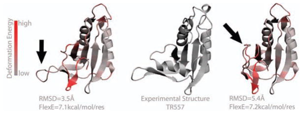
Example for two structural models corresponding to PDB code 2kyy (CASP code TR557, see SI table 1) where the two models have the same FlexE score but very different RMSDs. The arrow points at the area responsible for the large variation in RMSD score. FlexE assigns this area as flexible and therefore does not penalize this conformational change.

Third, Figure 7 shows a situation in which FlexE and RMSD disagree about which prediction is best. The leftmost structure has the lowest RMSD because of the good packing of the helix on top. However, FlexE does not “like” that structure, which is a β strand in the native structure. FlexE captures the energetic cost of breaking the hydrogens bond involved in the α-helix and forming the β-sheet.

Figure 7.

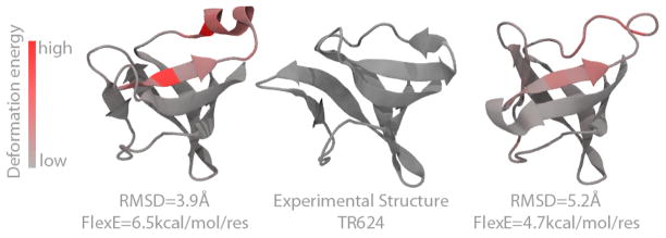
Example for two structural models corresponding to PDB code 3nrl (CASP code TR624, see SI table 1), here the model on the left despite having better RMSD has the wrong secondary structure (top helix) leading to high deformation energies.

4 FlexE compares protein structures by energies and complements comparisons by RMSDs

We have introduced FlexE, a computational method for comparing two structures of a protein. It computes an elastic deformation energy from one structure A to the other B based on the Elastic Network Model, but in principle, any other energy function could be used. Such comparisons give insights that can complement comparisons of structure that are based on geometric measures such RMSD or GDT-TS. We show ways that these methods are complementary. One example is a floppy loop. Suppose two researchers predict that loop to be in two different conformations. In a CASP event, the researcher finding the lowest RMSD would be judged best. But if the FlexE score shows the two loops have the same energy, it implies that both loop conformations are equally good. Or, suppose that two researchers predict two structures having the same RMSD to native. They would be judged to be equally good predictions. But, if they have very different FlexE scores, we show cases where we argue the better prediction is the one with the lower value of this energy score. In particular, we show that FlexE has the capability of recognizing when two structures are both true stable states of a protein versus when the two structures are generated by nonphysical processes. We believe FlexE will be useful for getting added insights when comparing protein structures.

References

- 1.Carugo O, Pongor S. Protein Sci. 2001;10:1470–1473. doi: 10.1110/ps.690101. [DOI] [PMC free article] [PubMed] [Google Scholar]
- 2.Damm KL, Carlson HA. Biophys J. 2006;90:4558–4573. doi: 10.1529/biophysj.105.066654. [DOI] [PMC free article] [PubMed] [Google Scholar]
- 3.Ye Y, Godzik A. Bioinformatics. 2003;19:ii246–ii255. doi: 10.1093/bioinformatics/btg1086. [DOI] [PubMed] [Google Scholar]
- 4.Zhang Y, Skolnick J. Nucleic Acids Research. 2005;33:2302–2309. doi: 10.1093/nar/gki524. [DOI] [PMC free article] [PubMed] [Google Scholar]
- 5.Sippl MJ, Wiederstein M. Bioinformatics. 2008;24:426–427. doi: 10.1093/bioinformatics/btm622. [DOI] [PubMed] [Google Scholar]
- 6.Kolodny R, Koehl P, Levitt M. J Mol Biol. 2005;346:1173– 1188. doi: 10.1016/j.jmb.2004.12.032. [DOI] [PMC free article] [PubMed] [Google Scholar]
- 7.Zemla A. Nucleic Acids Res. 2003;31:3370–3374. doi: 10.1093/nar/gkg571. [DOI] [PMC free article] [PubMed] [Google Scholar]
- 8.Moult J, Pedersen JT, Judson R, Fidelis K. Proteins: Struct, Funct, Bioinf. 1995;23:ii–iv. doi: 10.1002/prot.340230303. [DOI] [PubMed] [Google Scholar]
- 9.Tobi D, Bahar I. Proc Natl Acad Sci USA. 2005;102:18908–18913. doi: 10.1073/pnas.0507603102. [DOI] [PMC free article] [PubMed] [Google Scholar]
- 10.Wei BQ, Weaver LH, Ferrari AM, Matthews BW, Shoichet BK. J Mol Biol. 2004;337:1161– 1182. doi: 10.1016/j.jmb.2004.02.015. [DOI] [PubMed] [Google Scholar]
- 11.Ma J, Karplus M. Proc Natl Acad Sci USA. 1998;95:8502–8507. doi: 10.1073/pnas.95.15.8502. [DOI] [PMC free article] [PubMed] [Google Scholar]
- 12.Henzler-Wildman KA, Thai V, Lei M, Ott M, Wolf-Watz M, Fenn T, Pozharski E, Wilson MA, Petsko GA, Karplus M, Hubner CG, Kern D. Nature. 2007;450:838–844. doi: 10.1038/nature06410. [DOI] [PubMed] [Google Scholar]
- 13.Boehr DD, Nussinov R, Wright PE. Nat Chem Biol. 2009;5:789–796. doi: 10.1038/nchembio.232. [DOI] [PMC free article] [PubMed] [Google Scholar]
- 14.McCammon JA, Gelin BR, Karplus M. Nature. 1977;267:585–590. doi: 10.1038/267585a0. [DOI] [PubMed] [Google Scholar]
- 15.Brooks B, Karplus M. Proc Natl Acad Sci USA. 1983;80:6571–6575. doi: 10.1073/pnas.80.21.6571. [DOI] [PMC free article] [PubMed] [Google Scholar]
- 16.Atilgan AR, Durell SR, Jernigan RL, Demirel MC, Keskin O, Bahar I. Biophys J. 2001;80:505–15. doi: 10.1016/S0006-3495(01)76033-X. [DOI] [PMC free article] [PubMed] [Google Scholar]
- 17.Hinsen K. Bioinformatics. 2008;24:521–528. doi: 10.1093/bioinformatics/btm625. [DOI] [PubMed] [Google Scholar]
- 18.Kovacs JA, Chacon P, Abagyan R. Proteins: Struct, Funct, Bioinf. 2004;56:661–668. doi: 10.1002/prot.20151. [DOI] [PubMed] [Google Scholar]
- 19.Orellana L, Rueda M, Ferrer-Costa C, Lopez-Blanco JR, Chacon P, Orozco M. J Chem Theory Comput. 2010;6:2910–2923. doi: 10.1021/ct100208e. [DOI] [PubMed] [Google Scholar]
- 20.Kurkcuoglu O, Kurkcuoglu Z, Doruker P, Jernigan RL. Proteins: Struct, Funct, Bioinf. 2009;75:837–845. doi: 10.1002/prot.22292. [DOI] [PMC free article] [PubMed] [Google Scholar]
- 21.Rueda M, Chacon P, Orozco M. Structure. 2007;15:565– 575. doi: 10.1016/j.str.2007.03.013. [DOI] [PubMed] [Google Scholar]
- 22.Romo TD, Grossfield A. Proteins: Struct, Funct, Bioinf. 2011;79:23–34. doi: 10.1002/prot.22855. [DOI] [PubMed] [Google Scholar]
- 23.Gerstein M, Krebs W. Nucleic Acids Res. 1998;26:4280–4290. doi: 10.1093/nar/26.18.4280. [DOI] [PMC free article] [PubMed] [Google Scholar]
- 24.MacCallum JL, Perez A, Schnieders MJ, Hua L, Jacobson MP, Dill KA. Proteins: Struct, Funct, Bioinf. 2011;79:74–90. doi: 10.1002/prot.23131. [DOI] [PMC free article] [PubMed] [Google Scholar]
- 25.Rouse PE. J Chem Phys. 1953;21:1272–1280. [Google Scholar]
- 26.Hinsen K, Petrescu AJ, Dellerue S, Bellissent-Funel MC, Kneller GR. Chem Phys. 2000;261:25– 37. [Google Scholar]
- 27.Riccardi D, Cui Q, Phillips GN. Biophys J. 2009;96:464– 475. doi: 10.1016/j.bpj.2008.10.010. [DOI] [PMC free article] [PubMed] [Google Scholar]
- 28.Moritsugu K, Smith JC. Biophys J. 2007;93:3460– 3469. doi: 10.1529/biophysj.107.111898. [DOI] [PMC free article] [PubMed] [Google Scholar]
- 29.Yang L, Song G, Jernigan RL. Proc Natl Acad Sci USA. 2009;106:12347–12352. doi: 10.1073/pnas.0902159106. [DOI] [PMC free article] [PubMed] [Google Scholar]
- 30.Hinsen K, Thomas A, Field MJ. Proteins: Struct, Funct, Bioinf. 1999;34:369–382. [PubMed] [Google Scholar]
- 31.Lu M, Poon B, Ma J. J Chem Theory Comput. 2006;2:464–471. doi: 10.1021/ct050307u. [DOI] [PMC free article] [PubMed] [Google Scholar]
- 32.Bakan A, Meireles LM, Bahar I. Bioinformatics. 2011;27:1575–1577. doi: 10.1093/bioinformatics/btr168. [DOI] [PMC free article] [PubMed] [Google Scholar]
- 33.AMBER; version 10. University of California; San Francisco, CA: 2008. [Google Scholar]
- 34.Jorgensen WL, Chandrasekhar J, Madura JD, Impey RW, Klein ML. J Chem Phys. 1983;79:926–935. [Google Scholar]
- 35.Smith DE, Dang LX. J Chem Phys. 1994;100:3757–3766. [Google Scholar]
- 36.Aqvist J. J Phys Chem. 1990;94:8021–8024. [Google Scholar]
- 37.Darden T, York D, Pedersen L. J Chem Phys. 1993;98:10089–10092. [Google Scholar]
- 38.Cheatham TEI, Miller JL, Fox T, Darden TA, Kollman PA. J Am Chem Soc. 1995;117:4193–4194. [Google Scholar]
- 39.Ryckaert J, Ciccotti G, Berendsen H. J Comput Phys. 1977;23:327–341. [Google Scholar]
- 40.Godzik A. Protein Sci. 1996;5:1325–1338. doi: 10.1002/pro.5560050711. [DOI] [PMC free article] [PubMed] [Google Scholar]
- 41.Frauenfelder H, Sligar S, Wolynes P. Science. 1991;254:1598–1603. doi: 10.1126/science.1749933. [DOI] [PubMed] [Google Scholar]
- 42.Gerstein M, Lesk AM, Chothia C. Biochemistry. 1994;33:6739–6749. doi: 10.1021/bi00188a001. [DOI] [PubMed] [Google Scholar]
- 43.Daniel R, Dunn R, Finney J, Smith J. Annu Rev Biophys Biomol Struct. 2003;32:69–92. doi: 10.1146/annurev.biophys.32.110601.142445. [DOI] [PubMed] [Google Scholar]
- 44.Keskin O, Durell SR, Bahar I, Jernigan RL, Covell DG. Biophys J. 2002;83:663– 680. doi: 10.1016/S0006-3495(02)75199-0. [DOI] [PMC free article] [PubMed] [Google Scholar]
- 45.Meireles L, Gur M, Bakan A, Bahar I. Protein Sci. 2011;20:1645–1658. doi: 10.1002/pro.711. [DOI] [PMC free article] [PubMed] [Google Scholar]
- 46.Bahar I, Lezon TR, Yang LW, Eyal E. Annu Rev Biophys. 2010;39:23–42. doi: 10.1146/annurev.biophys.093008.131258. [DOI] [PMC free article] [PubMed] [Google Scholar]
- 47.MacCallum JL, Hua L, Schnieders MJ, Pande VS, Jacobson MP, Dill KA. Proteins: Struct, Funct, Bioinf. 2009;77:66–80. doi: 10.1002/prot.22538. [DOI] [PMC free article] [PubMed] [Google Scholar]
- 48.Dill K, Chan H. Nat Struct Biol. 1997;4:10–19. doi: 10.1038/nsb0197-10. [DOI] [PubMed] [Google Scholar]
Associated Data
This section collects any data citations, data availability statements, or supplementary materials included in this article.