A longitudinal comparison of hemodynamics and intraluminal thrombus deposition in abdominal aortic aneurysms

Abstract

Abdominal aortic aneurysm (AAA) is often accompanied by in traluminal thrombus (ILT), which complicates AAA progression and risk of rupture. Patient-specific computational fluid dynamics modeling of 10 small human AAA was performed to investigate relations between hemodynamics and ILT progression. The patients were imaged using magnetic resonance twice in a 2- to 3-yr interval. Wall content data were obtained by a planar T1-weighted fast spin echo black-blood scan, which enabled quantification of thrombus thickness at midaneurysm location during baseline and followup. Computational simulations with patient-specific geometry and boundary conditions were performed to quantify the hemodynamic parameters of time-averaged wall shear stress (TAWSS), oscillatory shear index (OSI), and mean exposure time at baseline. Spatially resolved quantifications of the change in ILT thickness were compared with the different hemodynamic parameters. Regions of low OSI had the strongest correlation with ILT growth and demonstrated a statistically significant correlation coefficient. Prominent regions of high OSI (>0.4) and low TAWSS (<1 dyn/cm²) did not appear to coincide with locations of thrombus deposition.

abdominal aortic aneurysm (AAA) is a permanent dilation (50% greater than the normal arterial wall diameter) of the abdominal aorta. The disease is progressive and fatal if untreated. Between 11,000 and 17,000 patients die annually in the United States (18a) from AAA rupture following progressive, often asymptomatic, enlargement, and only invasive treatments have proven effective at preventing rupture and premature death (13). Male gender, age, smoking, genetic factors, hypertension, and high cholesterol are among known risk factors (10), and diabetes is a negative risk factor (47). Degradation of the aortic wall, inflammation with immune responses, and biochemical wall stress are mechanisms that promote AAA initiation, influenced by molecular genetics (1). After the irreversible process of aneurysm formation, the dilated vessel creates an environment with complex blood flow and wall shear stress distribution (4, 5, 9, 14, 22, 37, 38), which is thought to perpetuate aneurysm progression.

The presence of intraluminal thrombus (ILT) complicates AAA growth. ILT is fibrin structure compound of platelets, blood cells, blood proteins, and cellular debris (20). ILT is more frequent in larger AAA since most patients develop thrombus as the aneurysm progresses. It has been proposed that platelets activate in regions of high shear and are subsequently advected towards the aneurysm wall where they accumulate in regions of low shear and form thrombus (8), with a possible role played by the vortical structures formed inside the aneurysm (9). It has also been shown that the flow field inside AAA may promote ILT formation by increasing residence time and trapping blood particles (7, 37, 38).

The effect of ILT on AAA progression and rupture remains controversial (48). ILT may deprive the aneurysm wall of oxygen, which may exacerbate wall inflammation and weakening (45). The rupture of ILT can lead to the rupture of the arterial wall (26), mature ILT can reduce the wall compliance (16) and increase dissection risk (42), and ILT growth rate can increase the likelihood of aneurysm rupture (35). However, it has been reported that ILT can reduce the stresses acting on the wall of the aneurysm (11, 46).

Patient-specific AAA blood flow modeling is a promising tool that may provide important information for understanding hemodynamic factors involved in AAA progression and potentially data for clinical decision making. The goal of the present work is to investigate potential hemodynamic factors that may lead to progression of thrombus inside AAA. In this study, quantifications of time-averaged wall shear stress (TAWSS), oscillatory shear index (OSI), and mean exposure time (MET) at the luminal surface are compared with thrombus accumulation from longitudinal in vivo midaneurysm magnetic resonance (MR) wall content data in patients with small AAA.

MATERIALS AND METHODS

Imaging.

Ten patients with small AAAs (diameter <5 cm) were recruited under a protocol approved by the Institutional Review Board at Stanford University, and each patient consented to participate in imaging at baseline and followup visits. Patient information, including the followup interval, is shown in Table 1. The geometric characteristics of the patients are shown in Table 2.

Table 1.

Patient information

Patient No.	Gender	Age at Baseline, yr	Followup Interval, mo	BMI	Smoked, yr	Quit Smoking, yr ago	HTN	DM
1	M	73	36	30.10	5	48	Y	—
2	M	60	44	29.45	48	7	Y	—
3	M	66	24	26.39	30	20	Y	—
4	M	73	24	30.48	6	48	Y	—
5	M	62	38	29.16	15	31	—	—
6	M	61	36	30.38	18	23	Y	—
7	M	73	31	27.67	0	—	—	—
8	M	69	30	27.97	52	4	Y	—
9	F	78	16	26.63	8	30	Y	—
10	M	72	22	30.72	45	15	Y	Y

DM, type 2 diabetes mellitus; HTN, hypertension; BMI, body mass index; M, male; F, female; Y, yes.

Table 2.

Geometric characteristics of aneurysms

	P1	P2	P3	P4	P5	P6	P7	P8	P9	P10
Maximum lumen diameter	3.26	2.61	3.07	3.62	3.08	3.00	2.97	2.29	3.42	4.08
Centerline length	8.82	4.49	8.76	5.85	7.79	5.92	6.43	7.25	4.47	9.12
Lumen volume	45.3	18.9	39.8	34.1	46.2	26.1	25.9	26.1	24.5	60.5

Lumen diameter is based on equivalent area diameter. Centerline length starts and ends when the aneurysm diameter is 10% larger than the native aorta. All units are based on cm. P–P10, patients 1–10.

During the baseline visit, aortic lumen, blood flow, and wall content data were collected. Patients were scanned with contrast-enhanced MR angiography (MRA) in the supine position with a 1.5 T Signa MR scanner (GE Healthcare, Waukesha, WI). A three-dimensional fast gradient echo MRA sequence was used to image the aortic lumen. The scan parameters for MRA included 3.0- to 3.3-ms repetition time, 0.7- to 0.8-ms echo time, 25° 77 flip angle, 3-mm thickness with 1.5-mm overlap, and 40 × 40 cm² field of view with 512 × 192 acquisition matrix per slice (reconstructed to 512 × 512). A single component phase contrast MR sequence (PCMRI) was used to acquire blood flow velocity at the cross sections of the supraceliac and infrarenal aorta. The scan parameters included 11.9- to 12.7-ms repetition time, 4.5- to 5.3-ms echo time, 20° 83 flip angle, 256 × 192 acquisition matrix per slice (reconstructed to 256 × 256), and 150 cm/s through-plane encoding velocity with 24 time point reconstruction. Afterward, a T1-weighted, double-inversion recovery fast spin echo sequence (black blood MR) was used to image the aortic wall contents on the oblique axial plane at the level of maximal aortic dilatation. The single slice acquisition reduced the acquisition time while patients held their breaths. The scan parameters included 42-ms echo time, 6-mm slice thickness, and 34 × 34 cm² field of view with 320 × 320 acquisition matrix per slice. All images were acquired during inspiratory breath hold to minimize the motion artifact. Brachial systolic and diastolic blood pressures were measured using an automatic pressure cuff (Omron Healthcare, Bannockburn, IL). During the followup visit, aortic lumen angiography and black blood MR scans were collected using consistent imaging sequences.

Image-based modeling.

Computer models of the aneurysm and surrounding arteries were created by segmenting the arterial lumina from the MRA data using the software package SimVascular (simtk.org/home/simvascular). The geometric models included the abdominal aorta with celiac trunk, superior mesenteric artery, renal arteries, and iliac arteries. The models were used as the domains for direct numerical simulation of the blood flow through the aneurysms, using methods similar to those described by Les et al. (22). The structural mechanics of the thrombus or aortic wall were not modeled. Blood was assumed to be an incompressible Newtonian fluid (ρ = 1.06 g/cm³, μ = 0.04 P). The Navier-Stokes equations were solved using a second-order accurate stabilized finite element method (21, 40). The method involves addition of stabilization terms to the Galerkin formulation of the Navier-Stokes equations to overcome instabilities in velocity due to presence of advection terms and instabilities in pressure due to the equal order pressure and velocity formulation used. The equal order interpolation results in continuous linear velocity and pressures on each element. A semidiscrete approach was used to discretize the spatial domain and integrate the resulting ordinary differential equations in time using a second order generalized-α method (21). A preconditioning method suitable for cardiovascular finite element simulations was used to increase the efficiency of the linear solver (17).

For the inflow boundary condition the supraceliac volumetric flow rate of each patient from PCMRI data were mapped to a Womerseley profile at the respective model's inlet. While the in vivo profile at the supraceliac aorta likely deviates from a Womerseley profile, imposing the profile at the supraceliac level ensures sufficient length for the flow to develop so that flow features at the infrarenal segment are not sensitive to the profile at the supraceliac level (4, 39).

For the outflow boundary condition, three-element (RCR) Windkessel models were imposed at the outlets using the coupling described by Vignon-Clementel et al. (44). To configure the flow rate to each vessel outlet, suprarenal and infrarenal PCMRI data were used to compute expected flow rates to branch vessels. Supraceliac minus infrarenal flow was distributed as 33.0% to the celiac trunk and 67% evenly to the superior mesenteric artery and renal arteries (27). Infrarenal flow was split equally between iliac arteries, and subsequently 70% of common iliac flow was distributed to the external iliac and 30% to the internal iliac arteries. The total resistance at each outlet (R_tot) was set to the patient's mean brachial pressure divided by the expected flow rate of the outlet. The resistance ratio R_p/R_tot was set to be 5.6% (28% for the renal arteries to avoid retrograde diastolic flow) (22), which enabled the calculation of the proximal (R_p) and distal (R_d) resistances, where R_tot = R_p + R_d. For determining compliance values, the total arterial compliance was obtained by the pulse pressure method (36) and distributed to the outlets according to the anticipated flow rate.

The models were meshed with anisotropic linear tetrahedral finite elements, with the maximum edge size of 0.075 cm, based on prior convergence studies using similar models (22). In addition, five layers of boundary layer meshing, with a next to wall edge size of 0.025 cm, were performed along all walls for accurate WSS computation. Qualitative comparison of WSS patterns to a mesh with maximum edge size of 0.05 cm in the interior and a next to wall edge size of 0.01 cm in the boundary layers was performed to ensure mesh convergence of WSS metrics. The simulation time step of the solver was set to divide the cardiac cycle into 1,000 to 2,000 time steps as needed to produce acceptable root mean square errors. The first two cycles were discarded, and the four subsequent cycles were used for quantitative analysis. The solution was converged after the first two cycles, as verified by the periodicity of velocity and WSS patterns.

Hemodynamics analysis.

Wall shear stress was quantified using two standard parameters, the TAWSS (defined as the magnitude of the vectorial average), and OSI. Four cardiac cycles were used in these computations, which was sufficient for convergence of results. Specifically, the TAWSS was calculated as

$$\text{TAWSS}=\Vert \frac{1}{4T}{\int }_0^{4T}{\overrightarrow{\tau }}_{\mathrm{w}\mathrm{a}\mathrm{l}\mathrm{l}}\hspace{0.17em}\text{d}t\Vert$$ (1)

The OSI was calculated to measure oscillation of the wall shear stress vector from its mean direction as

$$\text{OSI}=\frac{1}{2}\left(1-\frac{\Vert \frac{1}{4T}{\displaystyle {\int }_0^{4T}{\overrightarrow{\tau }}_{\mathrm{w}\mathrm{a}\mathrm{l}\mathrm{l}}\hspace{0.17em}\text{d}t}\Vert }{\frac{1}{4T}{\displaystyle {\int }_0^{4T}\left|{\overrightarrow{\tau }}_{\mathrm{w}\mathrm{a}\mathrm{l}\mathrm{l}}\right|\hspace{0.17em}\text{d}t}}\right)$$ (2)

Flow stagnation was quantified using the MET (23). The MET of each element in the flow solver mesh was measured as the accumulated amount of time that Lagrangian fluid particles entering the model spent inside model elements

$$\text{MET}(e)=\frac{1}{N_e\sqrt[3]{V_e}}{\displaystyle \sum _{p=1}^{N_p}{\displaystyle {\int }_0^{\infty }{H}_e(p,t)\hspace{0.17em}\text{d}t,}}\hspace{0.17em}\hspace{0.17em}{H}_e=\{\begin{array}{l}1\hspace{0.17em}\text{if}\hspace{0.17em}{x}_{\text{p}}(t)\in e\\ 0\hspace{0.17em}\text{if}\hspace{0.17em}{x}_{\text{p}}(t)\notin e\end{array}$$ (3)

where N_p is the total number of particles released, N_e is the number of encounters of a particle into the element e, V_e is the volume of the element, x_p(t) is the position of the particle, and H_e is the indicator function of the element e. MET by definition, measures both stagnation and recirculation, while weighing recirculation lower. To compute MET, particles were uniformly seeded (200-μm spacing) and released proximal to the aneurysm continuously over time. Namely, the particles were released in a way to maintain a uniform influx density by releasing based on local space-time flow rate for a total of four cardiac cycles. This created ∼10 million released particles. The particles were integrated for an additional eight cardiac cycles so that nearly all particles were flushed, and hence the indefinite integral in Eq. 3 could be truncated. The velocity data were assumed to be periodic after the sixth computed cardiac cycle to enable integration beyond the available data.

Wall content and thrombus quantification.

Thrombus thickness was quantified from the black blood MR images. Segmentations were performed using ITK-Snap (49). The black blood MR is prone to reduced signal-to-noise ratio in the region of low blood flow, which could lead to artifacts that were difficult to distinguish from thrombus. Therefore, the MRA for model construction was used to confirm lumen boundary from the black blood MR images. An axial plane of the MRA was chosen that matched as close as possible by visual inspection the axial plane of the black blood MR data. This allowed the lumen to be more readily identified or confirmed, and any intraluminal artifact in the black blood MR data discounted. Figure 1 displays both MRA and black blood MR data at baseline and followup for each patient. Patients 1, 3, 5, 6, and 10 did not have noticeable thrombus at the baseline or followup scan. Patients 4 and 7 did not have significant thrombus during the baseline scan, patient 8 had minimal thrombus progression from baseline to followup, and patients 2 and 9 had significant thrombus in both scans with notable progression.

Fig. 1.

Axial view of black (left) and bright (right) blood MR at location of maximum aneurysm diameter for each patient. The black blood MR enables better visualization of soft tissue and thrombus burden, and the bright blood MRA enables better visualization the aortic lumen. P1–P10, patients 1–10.

To quantify thrombus progression, a reference point on the spine was chosen from the baseline and followup image data. An angle θ was measured from the line connecting the center of the lumen to this reference point (Fig. 2). Thrombus thickness was measured as the distance between the lumen and the outer wall as a function of θ in the lumen-centered coordinate frame. Then, the change in thrombus thickness was obtained as the difference between thrombus thickness at followup and baseline at the same θ locations. A similar procedure was used to quantify the various hemodynamic parameters described above as a function of θ. For the hemodynamic parameters, values were locally averaged from a 1.4-cm thick annular luminal section, which was nominally centered on the axial slice of the black blood MR scan. Once thrombus thickness and the respective hemodynamic parameters were obtained as a function of θ, the θ variable was eliminated between the two functions to enable the hemodynamic parameters to be plotted against the quantified thrombus growth. A Gaussian filter was used to remove the high-frequency changes introduced due to this elimination, which did not affect the overall trend of the results.

Fig. 2.

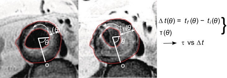
The procedure for quantifying thrombus thickness growth Δt as a function of θ. The hemodynamic parameters are also quantified similarly [time-averaged wall shear stress (TAWSS), oscillatory shear index (OSI), and mean exposure time (MET)].

RESULTS

The fields used to quantify the hemodynamics are shown in Figs. 3, 4, and 5. The approximate location of the plane where the planar black blood MR imaging was performed is indicated by the arrows. Figure 3 displays the TAWSS results. The entirety of the three-dimensional computer models is displayed in Fig. 3, whereas closer views of the aneurysmal segments are provided in Figs. 4 and 5. Most of the patients that did not develop thrombus have notable regions of very low (<1 dyn/cm²) TAWSS at the aneurysm bulge. Figure 4 displays the OSI fields. Most patients that demonstrated no thrombus deposition had significant regions of higher OSI. The MET results are displayed in Fig. 5. While MET was computed for all elements, Fig. 5 displays MET for the boundary elements only.

Fig. 3.

TAWSS for the 10 patients. The anterior (right) and posterior (left) views are shown. The arrows in the anterior view indicate the approximate plane where the black blood MR image data were acquired.

Fig. 4.

OSI for the 10 patients. The anterior (right) and posterior (left) views are shown. The arrows in the anterior view indicate the approximate plane where the black blood MR image data were acquired.

Fig. 5.

MET for the 10 patients for the elements on the boundary. The anterior (right) and posterior (left) views are shown. The arrows in the anterior view indicate the approximate plane where the black blood MR image data were acquired.

Quantification of thrombus growth vs. the hemodynamic parameters, for patients that had thrombus progression from baseline to followup, is plotted in Fig. 6. Note, Gaussian filtering preserves boundary information more than the other parts, resulting in less removal of high frequency variations near the ends of each plot. Thrombus growth was mostly observed in regions with TAWSS between 2 and 3 dyn/cm². OSI had a significant negative correlation with thrombus deposition, i.e., there is an increase in thrombus thickness in regions of lower OSI. No obvious correlation was found for MET of the boundary elements. Table 3 shows the Pearson's correlation coefficient calculated from the hemodynamic parameters vs. change in thrombus thickness. The correlation for TAWSS did not have an acceptable P value due to the negative correlation for one of the patients, and MET had no consistent correlation.

Fig. 6.

Quantification of OSI, TAWSS (dyn/cm²), and MET (s) vs. thrombus thickness growth (mm) for the patients that had thrombus deposition between baseline to followup. Note that the abscissa (change in thickness) changes between patients.

Table 3.

Pearson's correlation coefficient obtained from correlating different hemodynamic parameters with thrombus growth

Parameter	Patient 2	Patient 4	Patient 7	Patient 8	Patient 9	P Value
OSI	−0.96	−0.98	−0.94	−0.80	−0.72	6.8e-5
TAWSS	0.96	0.99	0.80	0.82	−0.74	0.16
MET	0.20	−0.70	0.91	−0.88	0.30	0.93

OSI, oscillatory shear index; TAWSS, time-averaged wall shear stress; MET, mean exposure time.

A size field on the lumen surface was quantified by calculating the distance from centerline to each point on the lumen. This was done for baseline and followup models to visualize the aneurysm growth. The centerline was calculated using vascular modeling toolkit (VMTK) (3). Figure 7 displays the distance from centerline during baseline and followup scans.

Fig. 7.

Distance (cm) between centerline and lumen surface at baseline scan (left) and followup scan (right) for each patient.

DISCUSSION

Thrombosis is a highly complex process involving various biochemical, biomechanical, and biophysical factors. This study investigated hemodynamic features in small AAA to explore possible relations to the development of ILT. Our finding was that OSI appeared to be a significant factor influencing thrombus deposition among the factors studied. Thrombus deposition occurred in regions where OSI was low compared with the surrounding, and generally patients who had noticeable regions of relatively high OSI did not have thrombus deposition. These regions of high OSI often, but not always, coincided with regions of low TAWSS (<1 dyn/cm²). While OSI is normalized to have value ranging from 0 to 0.5, values of TAWSS are more ambiguous. The range chosen for TAWSS here was set to 5 dyn/cm² to better stratify values. This enabled us to distinguish between regions of relatively low TAWSS (2–3 dyn/cm²) where deposition occurred and regions of lowest TAWSS (<1 dyn/cm²) where thrombus progression was mostly absent, perhaps due to higher OSI in such regions.

Thrombosis is governed by proteins originating locally and from platelets and proteins originating upstream. Our near-wall MET computation was geared toward measuring how long particles (platelets) entering the aneurysm from upstream were trapped near the wall (lumen surface). This was based on the hypothesis that thrombus in AAA is due (at least in part) to upstream platelets entering the aneurysm, becoming mechanically activated and subsequently becoming trapped in regions of high stagnation (8). However, our MET results do not support this hypothesis. Alternatively, biochemical activation may be more important, as well as the transport of chemicals and proteins from the wall. These species depend strongly on local concentrations and reaction rates and care must be taken in how such species are introduced into the model. Therefore, considerations of stagnation, such as measured using MET, are likely most relevant in conjunction with models coupling biochemical reaction with transport.

The conclusion that OSI was negatively correlated with thrombus deposition may be considered contrary to prevailing theory. High OSI, which indicates flow with no preferred direction, is commonly thought to be an adverse hemodynamic condition in atherosclerosis (41). While flow through a healthy aorta (during systole) may be generally considered attached and unidirectional, flow in AAA is generally separated (5, 22, 31, 33, 37). Under such conditions, low OSI may indicate regions of persistent reverse or recirculating flow, which may be prothrombotic. Regions of separated flow with higher OSI may indicate higher near wall mixing, which may help to prevent thrombus growth in regions of separated flow. These results motivate further investigation regarding the role of mixing in relation to chemical and cellular transport in AAA.

In prior comparisons of wall shear with thrombosis, Turitto and Baumgartner (43) observed an increase in platelet adhesion and thrombus formation with wall shear rate in vitro. Badimon et al. (6) studied the exposure of collagen, as well as deendothelialized aorta, to different wall shear rates. In both applications, an increase in wall shear rate caused an increase in platelet deposition. In the deendothelialized vessel, platelet deposition increased initially with an increase in exposure time but remained relatively unchanged for longer exposure times. The vessel wall conditions in their study represent an injured vessel wall, which may be considered relevant to AAA. These studies support the positive correlation of wall shear stress and thrombus formation found herein, although this finding was only modestly significant (P = 0.16). This correlation is potentially due to the higher rate of delivery of platelets at locations of (relatively) higher wall shear. This mechanism can promote thrombus formation through an increase in adhesion and aggregation of platelets flowing on the injured wall (2). It should be noted that shear stress levels throughout AAA are generally lower than in the healthy abdominal aorta. Hence, it is the relative difference in shear rather than absolute values that are of relevance here. We note that temporal and spatial gradients of WSS could potentially be correlated with thrombus deposition. However, we have observed that these measures have high positive correlation with WSS magnitude, which limits useful independent information from these measures.

Prior investigations have shown flow reversal at the wall may increase monocyte adhesion (12), and flow recirculation is positively correlated with thrombosis biomarkers (25). Consistently, we observed that persistent regions of recirculation contribute to low OSI and enhanced thrombus deposition. In a recent computational study of AAA (28), OSI was found to be negatively correlated to thrombus deposition. We also note that the theory linking low, and oscillatory, WSS with atherosclerosis has recently been challenged (29), with the authors pointing out that such correlations have not been found in studies performing point-wise comparisons.

Identification of prothrombotic hemodynamic conditions is desirable since thrombus growth rate may be a predictor of rupture (35). This study supports the possibility that thrombus deposition could be potentially predicted with a patient-specific framework. However, due to the complexities involved in thrombosis, the identification of a single hemodynamic surrogate to predict thrombus accumulation is tenuous. Previous studies (8) have mentioned that low WSS cannot be the only hemodynamic parameter related to thrombus deposition due to the lower WSS observed in saccular aneurysms, which are more frequently thrombus free. Our investigations have shown that the regions of very low TAWSS (<1 dyn/cm²) are generally accompanied by high OSI and do not favor thrombus deposition.

Limitations.

The main modeling assumptions used in this work were that macroscopic blood flow dynamics could be effectively recovered using a Newtonian fluid model and a no slip (zero velocity) condition on the lumen. Employing more sophisticated models for the blood rheology, or wall mechanics, is in theory possible, but without proper patient-specific data such models may not provide more accurate modeling of in vivo blood flow conditions (34). Nevertheless, the flow field inside complex vascular geometries such as AAA is generally dominated by the local lumen morphology and inflow/outflow boundary conditions, with blood rheology and fluid-structure interactions having a relatively smaller effect on macroscopic flow conditions (34). Changes in AAA hemodynamics between a Newtonian and a non-Newtonian model have been investigated (9), but differences in WSS did not appear compelling. Difference in hemodynamics due to wall motion have also been investigated (15) and found to be negligible when radial strains were less than ≈8%. Radial strains were observed to be <5% from the PCMRI data for the AAAs considered.

The presence of ILT in computational modeling of AAA wall has been shown to be an important factor altering wall stress distributions (18, 24, 46). From the fluid mechanics point of view, the presence of ILT can alter the flow field in different ways. ILT alters lumen morphology. This is expected to be the most significant effect and has been accounted for in this study. ILT can also alter the mechanical properties of fluid structure interaction; however, such interactions were not considered for reasons stated above. The porous nature of ILT may question the no-slip (no-penetration) boundary condition used on the wall. How significant this change can be to the flow field patterns is something that is not clearly known and requires further investigation.

Our measurement of thrombus growth was limited by challenges that arose from coregistration of baseline and followup image data. The lumen-centered coordinate choice used herein for quantifying thrombus thickness and hemodynamics data on the midaneurysm plane is not expected to provide precise registration, and there is uncertainty in axial slice location between the three scans used in our analysis (i.e., the hemodynamics data based on baseline MRA image coordinates, thrombus thicknesses based on baseline black blood MR coordinates, and thrombus thickness based on followup black blood MR coordinates). The induced errors are difficult to quantify. The former problem manifests in, among other things, potentially different θs between baseline thickness, baseline hemodynamic parameter and followup thickness. To help reduce these errors, a Gaussian filter was applied once θ was eliminated. However, the unfiltered data still produced Pearson correlations consistently negative for OSI (between −0.6 to −0.8 for most patients) and maintained statistical significance. To help alleviate potential differences in axial plane locations, we performed averaging of the hemodynamics data over a thin annular band and confirmed that our results were insensitive to the chosen thickness (1.4 cm). Moreover, an interobserver study was performed on two of the patients (patients 4 and 8) to examine the sensitivity of the calculated correlation coefficients due to variability of segmentations between blinded operators. This comparison yielded all correlation coefficients changing <3%. In this study the full three-dimensional progression of thrombus was not known, and the approach presented here could benefit by being extended to multiple slices in studies where such data are available. Moreover, the small number of patients that developed thrombus in this study is another limitation, and a larger number of patients would be desirable for more definite conclusions.

Conclusions.

Patient-specific modeling of blood flow in 10 patients with small AAA was compared with ILT growth from a 2- to 3-yr followup. The results indicated that regions of low OSI were the most vulnerable for thrombus growth, demonstrating a statistically significant negative Pearson correlation coefficient. TAWSS did not indicate a strong correlation with thrombus deposition but generally demonstrated a positive correlation. Prominent regions of high OSI (>0.4) and very low TAWSS (<1 dyn/cm²) appeared to not promote thrombus deposition.

GRANTS

This work was supported by National Heart, Lung, and Blood Institute Grant 5R21-HL-108272. Patient recruitment and medical data collection were supported by National Institutes of Grants P50-HL-083800 and P41-RR-09784, Veterans Affairs Palo Alto Health Care System, and Lucas Center for Magnetic Resonance Imaging at Stanford.

DISCLOSURES

No conflicts of interest, financial or otherwise, are declared by the author(s).

AUTHOR CONTRIBUTIONS

Author contributions: A.A. and S.C.S. conception and design of research; A.A. and G.-Y.S. performed experiments; A.A., G.-Y.S., and S.C.S. analyzed data; A.A. and S.C.S. prepared figures; A.A. and S.C.S. drafted manuscript; A.A., G.-Y.S., R.L.D., and S.C.S. edited and revised manuscript; A.A., G.-Y.S., R.L.D., and S.C.S. approved final version of manuscript; R.L.D. and S.C.S. interpreted results of experiments.

REFERENCES

- 1.Ailawadi G, Eliason JL, Upchurch GR. Current concepts in the pathogenesis of abdominal aortic aneurysm. J Vasc Surg 38: 584–588, 2003. [DOI] [PubMed] [Google Scholar]
- 2.Alevriadou BR, Moake JL, Turner NA, Ruggeri ZM, Folie BJ, Phillips MD, Schreiber AB, Hrinda ME, McIntire LV. Real-time analysis of shear-dependent thrombus formation and its blockade by inhibitors of von Willebrand factor binding to platelets. Blood 81: 1263–1276, 1993. [PubMed] [Google Scholar]
- 3.Antiga L, Piccinelli M, Botti L, Ene-Iordache B, Remuzzi A, Steinman DA. An image-based modeling frame work for patient-specific computational hemodynamics. Med Biol Eng Comput 46: 1097–1112, 2008. [DOI] [PubMed] [Google Scholar]
- 4.Arzani A, Les AS, Dalman RL, Shadden SC. Effect of exercise on patient specific abdominal aortic aneurysm flow topology and mixing. Int J Numer Method Biomed Eng 30: 280–295, 2014. [DOI] [PMC free article] [PubMed] [Google Scholar]
- 5.Arzani A, Shadden SC. Characterization of the transport topology in patient-specific abdominal aortic aneurysm models. Phys Fluids 24: 1901, 2012. [DOI] [PMC free article] [PubMed] [Google Scholar]
- 6.Badimon L, Badimon JJ, Galvez A, Chesebro JH, Fuster V. Influence of arterial damage and wall shear rate on platelet deposition. Ex vivo study in a swine model. Arterioscler Thromb Vasc Biol 6: 312–320, 1986. [DOI] [PubMed] [Google Scholar]
- 7.Basciano C, Kleinstreuer C, Hyun S, Finol EA. A relation between near-wall particle-hemodynamics and onset of thrombus formation in abdominal aortic aneurysms. Ann Biomed Eng 39: 2010–2026, 2011. [DOI] [PMC free article] [PubMed] [Google Scholar]
- 8.Biasetti J, Gasser TC, Auer M, Hedin U, Labruto F. Hemodynamics of the normal aorta compared with fusiform and saccular abdominal aortic aneurysms with emphasis on a potential thrombus formation mechanism. Ann Biomed Eng 38: 380–390, 2010. [DOI] [PubMed] [Google Scholar]
- 9.Biasetti J, Hussain F, Gasser TC. Blood flow and coherent vortices in the normal and aneurysmatic aortas: a fluid dynamical approach to intra-luminal thrombus formation. J R Soc Interface 8: 1449–1461, 2011. [DOI] [PMC free article] [PubMed] [Google Scholar]
- 10.Blanchard J. Epidemiology of abdominal aortic aneurysms. Epidemiol Rev 21: 207–221, 1999. [DOI] [PubMed] [Google Scholar]
- 11.Bluestein D, Dumont K, De Beule M, Ricotta J, Impellizzeri P, Verhegghe B, Verdonck P. Intraluminal thrombus and risk of rupture in patient specific abdominal aortic aneurysm–FSI modelling. Comput Methods Biomech Biomed Engin 12: 73–81, 2009. [DOI] [PubMed] [Google Scholar]
- 12.Conway DE, Williams MR, Eskin SG, McIntire LV. Endothelial cell responses to atheroprone flow are driven by two separate flow components: low time-average shear stress and fluid flow reversal. Am J Physiol Heart Circ Physiol 298: H367–H374, 2010. [DOI] [PMC free article] [PubMed] [Google Scholar]
- 13.Dalman RL, Tedesco MM, Myers J, Taylor CA. AAA disease. Ann NY Acad Sci 1085: 92–109, 2006. [DOI] [PubMed] [Google Scholar]
- 14.Deplano V, Knapp Y, Bertrand E, Gaillard E. Flow behaviour in an asymmetric compliant experimental model for abdominal aortic aneurysm. J Biomech 40: 2406–2413, 2007. [DOI] [PubMed] [Google Scholar]
- 15.Duvernois V, Marsden AL, Shadden SC. Lagrangian analysis of hemodynamics data from FSI simulation. Int J Numer Method Biomed Eng 29: 445–461, 2013. [DOI] [PMC free article] [PubMed] [Google Scholar]
- 16.Ene F, Gachon C, Delassus P, Carroll R, Stefanov F, O'Flynn P, Morris L. In vitro evaluation of the effects of intraluminal thrombus on abdominal aortic aneurysm wall dynamics. Med Eng Phys 33: 957–966, 2011. [DOI] [PubMed] [Google Scholar]
- 17.Esmaily-Moghadam M, Bazilevs Y, Marsden AL. A new preconditioning technique for implicitly coupled multidomain simulations with applications to hemodynamics. Comput Mech 52: 1141–1152, 2013. [Google Scholar]
- 18.Gasser TC, Auer M, Labruto F, Swedenborg J, Roy J. Biomechanical rupture risk assessment of abdominal aortic aneurysms: model complexity vs. predictability of finite element simulations. Eur J Vasc Endovasc Surg 40: 176–185, 2010. [DOI] [PubMed] [Google Scholar]
- 18a.Go AS, Mozaffarian D, Roger VL, Benjamin EJ, Berry JD, Borden WB, Bravata DM, Dai S, Ford ES, Fox CS, Franco S, Fullerton HJ, Gillespie C, Hailpern SM, Heit JA, Howard VJ, Huffman MD, Kissela BM, Kittner SJ, Lackland DT, Lichtman JH, Lisabeth LD, Magid D, Marcus GM, Marelli A, Matchar DB, McGuire DK, Mohler ER, Moy CS, Mussolino ME, Nichol G, Paynter NP, Schreiner PJ, Sorlie PD, Stein J, Turan TN, Virani SS, Wong ND, Woo D, Turner MB; American Heart Association Statistics Committee and Stroke Statistics Subcommittee. Heart disease and stroke statistics–2013 update: a report from the American Heart Association. Circulation 127: e6–e245, 2013. [DOI] [PMC free article] [PubMed] [Google Scholar]
- 19.Hardman D, Semple SI, Richards JM, Hoskins PR. Comparison of patient-specific inlet boundary conditions in the numerical modelling of blood flow in abdominal aortic aneurysm disease. Int J Numer Method Biomed Eng 29: 165–178, 2013. [DOI] [PubMed] [Google Scholar]
- 20.Harter LP, Gross BH, Callen PW, Barth RA. Ultrasonic evaluation of abdominal aortic thrombus. J Ultrasound Med 1: 315–318, 1982. [DOI] [PubMed] [Google Scholar]
- 21.Jansen KE, Whiting CH, Hulbert GM. A generalized-alpha method for integrating the filtered Navier-Stokes equations with a stabilized finite element method. Comput Methods Biomech Biomed Engin 190: 305–319, 2000. [Google Scholar]
- 22.Les AS, Shadden SC, Figueroa CA, Park JM, Tedesco MM, Herfkens RJ, Dalman RL, Taylor CA. Quantification of hemodynamics in abdominal aortic aneurysms during rest and exercise using magnetic resonance imaging and computational fluid dynamics. Ann Biomed Eng 38: 1288–1313, 2010. [DOI] [PMC free article] [PubMed] [Google Scholar]
- 23.Lonyai A, Dubin AM, Feinstein JA, Taylor CA, Shadden SC. New insights into pacemaker lead-induced venous occlusion: simulation-based investigation of alterations in venous biomechanics. Cardiovasc Eng 10: 84–90, 2010. [DOI] [PubMed] [Google Scholar]
- 24.Maier A, Gee MW, Reeps C, Pongratz J, Eckstein HH, Wall WA. A comparison of diameter, wall stress, and rupture potential index for abdominal aortic aneurysm rupture risk prediction. Ann Biomed Eng 38: 3124–3134, 2010. [DOI] [PubMed] [Google Scholar]
- 25.Martorell J, Santomá P, Kolandaivelu K, Kolachalama VB, Melgar-Lesmes P, Molins JJ, Garcia L, Edelman ER, Balcells M. Extent of flow recirculation governs expression of atherosclerotic and thrombotic biomarkers in arterial bifurcations. Cardiovasc Res 103: 37–46, 2014. [DOI] [PMC free article] [PubMed] [Google Scholar]
- 26.Martufi G, Gasser TC. Review: the role of biomechanical modeling in the rupture risk assessment for abdominal aortic aneurysms. J Biomech Eng 135: 021010, 2013. [DOI] [PubMed] [Google Scholar]
- 27.Moore JE, Jr, Ku DN. Pulsatile velocity measurements in a model of the human abdominal aorta under resting conditions. J Biomech Eng 116: 337–346, 1994. [DOI] [PubMed] [Google Scholar]
- 28.O'Rourke MJ, McCullough JP, Kelly S. An investigation of the relationship between hemodynamics and thrombus deposition within patient-specific models of abdominal aortic aneurysm. Proc Inst Mech Eng H 226: 548–564, 2012. [DOI] [PubMed] [Google Scholar]
- 29.Peiffer V, Sherwin SJ, Weinberg PD. Does low and oscillatory wall shear stress correlate spatially with early atherosclerosis? A systematic review. Cardiovasc Res 99: 242–250, 2013. [DOI] [PMC free article] [PubMed] [Google Scholar]
- 31.Salsac AV, Sparks SR, Chomaz JM, Lasheras JC. Evolution of the wall shear stresses during the progressive enlargement of symmetric abdominal aortic aneurysms. J Fluid Mech 560: 19–52, 2006. [Google Scholar]
- 32.Schmidt JP, Delp SL, Sherman MA, Taylor CA, Pande VS, Altman RB. The Simbios National Center: systems biology in motion. Proc IEEE Inst Electr Electron Eng 96: 1266–1280, 2008. [DOI] [PMC free article] [PubMed] [Google Scholar]
- 33.Shadden SC, Taylor CA. Characterization of coherent structures in the cardiovascular system. Ann Biomed Eng 36: 1152–1162, 2008. [DOI] [PMC free article] [PubMed] [Google Scholar]
- 34.Steinman DA. Assumptions in modelling of large artery hemodynamics. In: Modeling of Physiological Flows, edited by Ambrosi D, Quarteroni A, Rozza G. Milan, Italy: Springer, 2012, p. 1–18. [Google Scholar]
- 35.Stenbaek J, Kalin B, Swedenborg J. Growth of thrombus may be a better predictor of rupture than diameter in patients with abdominal aortic aneurysms. Eur J Vasc Endovasc Surg 20: 466–469, 2000. [DOI] [PubMed] [Google Scholar]
- 36.Stergiopulos N, Meister JJ, Westerhof N. Simple and accurate way for estimating total and segmental arterial compliance: the pulse pressure method. Ann Biomed Eng 22: 392–397, 1994. [DOI] [PubMed] [Google Scholar]
- 37.Suh GY, Les AS, Tenforde AS, Shadden SC, Spilker RL, Yeung JJ, Cheng CP, Herfkens RJ, Dalman RL, Taylor CA. Quantification of particle residence time in abdominal aortic aneurysms using magnetic resonance imaging and computational fluid dynamics. Ann Biomed Eng 39: 864–883, 2011. [DOI] [PMC free article] [PubMed] [Google Scholar]
- 38.Suh GY, Tenforde AS, Shadden SC, Spilker RL, Cheng CP, Herfkens RJ, Dalman RL, Taylor CA. Hemodynamic changes in abdominal aortic aneurysms with increasing exercise intensity using MR exercise imaging and image-based computational fluid dynamics. Ann Biomed Eng 39: 2186–2202, 2011. [DOI] [PMC free article] [PubMed] [Google Scholar]
- 39.Tang BT, Cheng CP, Draney MT, Wilson NM, Tsao PS, Herfkens RJ, Taylor CA. Abdominal aortic hemodynamics in young healthy adults at rest and during lower limb exercise: quantification using image-based computer modeling. Am J Physiol Heart Circ Physiol 291: H668–H676, 2006. [DOI] [PubMed] [Google Scholar]
- 40.Taylor CA, Hughes TJ, Zarins CK. Finite element modeling of blood flow in arteries. Comput Methods Biomech Biomed Engin 158: 155–196, 1998. [Google Scholar]
- 41.Taylor CA, Hughes TJ, Zarins CK. Finite element modeling of three-dimensional pulsatile flow in the abdominal aorta: relevance to atherosclerosis. Ann Biomed Eng 26: 975–987, 1998. [DOI] [PubMed] [Google Scholar]
- 42.Tong J, Cohnert T, Regitnig P, Kohlbacher J, Birner-Gruenberger R, Schriefl AJ, Sommer G, Holzapfel GA. Variations of dissection properties and mass fractions with thrombus age in human abdominal aortic aneurysms. J Biomech 47: 14–23, 2014. [DOI] [PubMed] [Google Scholar]
- 43.Turitto VT, Baumgartner HR. Platelet interaction with subendothelium in flowing rabbit blood: effect of blood shear rate. Microvasc Res 17: 38–54, 1979. [DOI] [PubMed] [Google Scholar]
- 44.Vignon-Clementel IE, Figueroa CA, Jansen KE, Taylor CA. Outflow boundary conditions for three-dimensional finite element modeling of blood flow and pressure in arteries. Comput Methods Biomech Biomed Engin 195: 3776–3796, 2006. [Google Scholar]
- 45.Vorp DA, Lee PC, Wang DH, Makaroun MS, Nemoto EM, Ogawa S, Webster MW. Association of intraluminal thrombus in abdominal aortic aneurysm with local hypoxia and wall weakening. J Vasc Surg 34: 291–299, 2001. [DOI] [PubMed] [Google Scholar]
- 46.Wang DH, Makaroun MS, Webster MW, Vorp DA. Effect of intraluminal thrombus on wall stress in patient-specific models of abdominal aortic aneurysm. J Vasc Surg 36: 598–604, 2002. [DOI] [PubMed] [Google Scholar]
- 47.Weiss JS, Sumpio BE. Review of prevalence and outcome of vascular disease in patients with diabetes mellitus. Eur J Vasc Endovasc Surg 31: 143–150, 2006. [DOI] [PubMed] [Google Scholar]
- 48.Wilson JS, Virag L, Di Achille P, Karsaj I, Humphrey JD. Biochemomechanics of intraluminal thrombus in abdominal aortic aneurysms. J Biomech Eng 135: 021011–021011, 2013. [DOI] [PMC free article] [PubMed] [Google Scholar]
- 49.Yushkevich PA, Piven J, Hazlett HC, Smith RG, Ho S, Gee JC, Gerig G. User-guided 3D active contour segmentation of anatomical structures: significantly improved efficiency and reliability. Neuroimage 31: 1116–1128, 2006. [DOI] [PubMed] [Google Scholar]