Single-shot compressed ultrafast photography at one hundred billion frames per second

Capturing transient scenes at a high imaging speed has been pursued by photographers for centuries^1–4, tracing back to Muybridge’s 1878 recording of a horse in motion⁵ and Mach’s 1887 photography of a supersonic bullet⁶. However, not until the late 20^th century were breakthroughs achieved in demonstrating ultra-high speed imaging (>100 thousand, or 10⁵, frames per second (fps))⁷. In particular, the introduction of electronic imaging sensors, such as the charge-coupled device (CCD) and complementary metal-oxide-semiconductor (CMOS), revolutionized high-speed photography, enabling acquisition rates up to ten million (10⁷) fps⁸. Despite these sensors’ widespread impact, further increasing frame rates using CCD or CMOS is fundamentally limited by their on-chip storage and electronic readout speed⁹. Here we demonstrate a two-dimensional (2D) dynamic imaging technique, compressed ultrafast photography (CUP), which can capture non-repetitive time-evolving events at up to 100 billion (10¹¹) fps. Compared with existing ultrafast imaging techniques, CUP has a prominent advantage of measuring an x, y, t (x, y, spatial coordinates; t, time) scene with a single camera snapshot, thereby allowing observation of transient events occurring on a time scale down to tens of picoseconds. Further, akin to traditional photography, CUP is receive-only—avoiding specialized active illumination required by other single-shot ultrafast imagers^2,3. As a result, CUP can image a variety of luminescent—such as fluorescent or bioluminescent—objects. Using CUP, we visualise four fundamental physical phenomena with single laser shots only: laser pulse reflection, refraction, photon racing in two media, and faster-than-light propagation of non-information. Given CUP’s capability, we expect it to find widespread applications in both fundamental and applied sciences including biomedical research.

To record events occurring at sub-nanosecond scale, currently the most effective approach is to use a streak camera, i.e., an ultrafast photo-detection system that transforms the temporal profile of a light signal into a spatial profile by shearing photoelectrons perpendicularly to their direction of travel with a time-varying voltage¹⁰. However, a typical streak camera is a one-dimensional (1D) imaging device—a narrow entrance slit (10 – 50 μm wide) limits the imaging field of view (FOV) to a line. To achieve 2D imaging, the system thus requires additional mechanical or optical scanning along the orthogonal spatial axis. Although this paradigm is capable of providing a frame rate fast enough to catch photons in motion^11,12, the event itself must be repetitive—following exactly the same spatiotemporal pattern—while the entrance slit of a streak camera steps across the entire FOV. In cases where the physical phenomena are either difficult or impossible to repeat, such as optical rogue waves¹³, nuclear explosion, and gravitational collapse in a supernova, this 2D streak imaging method is inapplicable.

To overcome this limitation, here we present CUP (Fig. 1), which can provide 2D dynamic imaging using a streak camera without employing any mechanical or optical scanning mechanism with a single exposure. On the basis of compressed sensing (CS)¹⁴, CUP works by encoding the spatial domain with a pseudo-random binary pattern, followed by a shearing operation in the temporal domain, performed using a streak camera with a fully opened entrance slit. This encoded, sheared three-dimensional (3D) x, y, t scene is then measured by a 2D detector array, such as a CCD, with a single snapshot. The image reconstruction process follows a strategy similar to CS-based image restoration^15–19 — iteratively estimating a solution that minimizes an objective function.

Fig. 1.

CUP system configuration. CCD, charge-coupled device; DMD, digital micromirror device; V, sweeping voltage; t, time. Since the DMD’s resolution pixel size (7.2 μm×7.2 μm) is much larger than the light wavelength, the diffraction angle is small (~ 4°). With a collecting objective of an NA = 0.16, the throughput loss caused by DMD’s diffraction is negligible.

By adding a digital micromirror device (DMD) as the spatial encoding module and applying the CUP reconstruction algorithm, we transformed a conventional 1D streak camera to a 2D ultrafast imaging device. The resultant system can capture a single, non-repetitive event at up to 100 billion fps with appreciable sequence depths (up to 350 frames per acquisition). Moreover, by using a dichroic mirror to separate signals into two colour channels, we expand CUP’s functionality into the realm of 4D x, y, t, λ ultrafast imaging, maximizing the information content that we can simultaneously acquire from a single instrument (Methods).

CUP operates in two steps: image acquisition and image reconstruction. The image acquisition can be described by a forward model (Methods). The input image is encoded with a pseudo-random binary pattern and then temporally dispersed along a spatial axis using a streak camera. Mathematically, this process is equivalent to successively applying a spatial encoding operator, C, and a temporal shearing operator, S, to the intensity distribution from the input dynamic scene, I(x, y, t):

$$I_s(x^{″},y^{″},t)=\mathit{SC}I(x,y,t),$$ (1)

where I_s(x″, y″, t) represents the resultant encoded, sheared scene. Next, I_s is imaged by a CCD, a process that can be mathematically formulated as

$$E(m,n)=\mathit{T}{I}_s(x^{″},y^{″},t).$$ (2)

Here, T is a spatiotemporal integration operator (spatially integrating over each CCD pixel and temporally integrating over the exposure time). E(m, n) is the optical energy measured at pixel m, n on the CCD. Substituting Eq. 1 into Eq. 2 yields

$$E(m,n)=\mathit{O}I(x,y,t),$$ (3)

where O represents a combined linear operator, i.e., O = TSC.

The image reconstruction is solving the inverse problem of Eq. 3. Given the operator O and spatiotemporal sparsity of the event, we can reasonably estimate the input scene, I(x, y, t), from measurement, E(m, n), by adopting a compressed-sensing algorithm, such as Two-Step Iterative Shrinkage/Thresholding (TwIST)¹⁶ (detailed in Methods). The reconstructed frame rate, r, is determined by

$$r=\frac{v}{\mathrm{\Delta }{y}^{″}}.$$ (4)

Here v is the temporal shearing velocity of the operator S, i.e., the shearing velocity of the streak camera, and Δy″ is the CCD’s binned pixel size along the temporal shearing direction of the operator S.

The CUP’s configuration is shown in Fig. 1. The object is first imaged by a camera lens with a focal length (F.L.) of 75 mm (Fujinon CF75HA-1). The intermediate image is then passed to a DMD (Texas Instruments DLP^® LightCrafter^™) by a 4-f imaging system consisting of a tube lens (F.L. = 150 mm) and a microscope objective (Olympus UPLSAPO 4×, F.L. = 45 mm, numerical aperture (NA) = 0.16). To encode the input image, a pseudo-random binary pattern is generated and displayed on the DMD, with a binned pixel size of 21.6 μm × 21.6 μm (3 × 3 binning).

The light reflected from the DMD is collected by the same microscope objective and tube lens, reflected by a beam splitter, and imaged onto the entrance slit of a streak camera (Hamamatsu C7700). To allow 2D imaging, this entrance slit is opened to its maximal width (~5 mm). Inside the streak camera, a sweeping voltage is applied along the y″ axis, deflecting the encoded image frames towards different y″ locations according to their times of arrival. The final temporally dispersed image is captured by a CCD (672 × 512 binned pixels (2 × 2 binning); Hamamatsu ORCA-R²) with a single exposure.

To characterise the system’s spatial frequency responses, we imaged a dynamic scene, a laser pulse impinging upon a stripe pattern with varying periods as shown in Fig. 2a. The stripe frequency (in line pairs/mm) descends stepwise along the x axis from one edge to the other. We shined a collimated laser pulse (532 nm wavelength, 7 ps pulse duration, Attodyne APL-4000) on the stripe pattern at an oblique angle of incidence α of ~30 degrees with respect to the normal of the pattern surface. The imaging system faced the pattern surface and collected the scattered photons from the scene. The impingement of the light wavefront upon the pattern surface was imaged by CUP at 100 billion fps with the streak camera’s shearing velocity set to 1.32 mm/ns. The reconstructed 3D x, y, t image of the scene in intensity (W/m²) is shown in Fig. 2b, and the corresponding time-lapse 2D x, y images (50 mm × 50 mm FOV; 150 × 150 pixels as nominal resolution) are provided in Supplementary Video 1.

Fig. 2.

Characterization of CUP’s spatial frequency responses. a. Experimental setup. A collimated laser pulse illuminates a stripe pattern obliquely. The CUP system faces the scene and collects the scattered photons. b. Reconstructed x, y, t datacube representing a laser pulse impinging upon the stripe pattern. In the representative frame for t = 60 ps, the dashed line indicates the light wavefront, and the arrow denotes the in-plane light propagation direction (k_xy). The entire temporal evolution of this event is shown in Supplementary Video 1. c. Reference image captured without introducing temporal dispersion. d–e. Projected vertical and horizontal stripe images calculated by summing over the x, y, t datacube voxels along the temporal axis. f. Comparison of average light fluence distributions along the x axis in c–d as well as along the y axis in e. G₁, G₂, G₃, and G₄ refer to the stripe groups with ascending spatial frequencies. g. Spatial frequency responses for five different orientations of the stripe pattern. The inner white dashed ellipse represents the CUP system’s band limit, and the outer yellow dash-dotted circle represents the band limit of the optical modulation transfer function without temporal shearing. Scale bars in b and g, 10 mm and 0.1 mm⁻¹, respectively.

Figure 2b also shows a representative temporal frame at t = 60 ps. Within a 10 ps exposure, the wavefront propagates 3 mm in space. Including the thickness of the wavefront itself, which is ~2 mm, the wavefront image is approximately 5 mm thick along the wavefront propagation direction. The corresponding intersection with the x-y plane is 5 mm/sinα ≈ 10 mm thick, which agrees with the actual measurement (~10 mm).

We repeated the light sweeping experiment at four additional angles of the stripe pattern (22.5°, 45°, 67.5°, and 90° with respect to the x axis) and also directly imaged the scene without temporal dispersion to acquire a reference (Fig. 2c). We projected the x, y, t datacubes onto the x, y plane by summing over the voxels along the temporal axis. The resultant images at two representative angles (0° and 90°) are shown in Figs. 2d and 2e, respectively. We compare in Fig. 2f the average light fluence (J/m²) distributions along the x axis from Fig. 2c and Fig. 2d as well as that along the y axis from Fig. 2e. The comparison indicates that CUP can recover spatial frequencies up to 0.3 line pairs/mm (groups G₁, G₂, and G₃) along both x and y axes; however, the stripes in group G₄—having a fundamental spatial frequency of 0.6 line pairs/mm—are beyond the CUP system’s resolution.

We further analysed the resolution by computing the spatial frequency spectra of the average light fluence distributions for all five orientations (Fig. 2g). Each angular branch appears continuous rather than discrete because the object has multiple stripe groups of varied frequencies and each has a limited number of periods. As a result, the spectra from the individual groups are broadened and overlapped. The CUP’s spatial frequency response band is delimited by the inner white dashed ellipse, whereas the band purely limited by the optical modulation transfer function of the system without temporal shearing—derived from the reference image (Fig. 2c)—is enclosed by the outer yellow dash-dotted circle. The CUP resolutions along the x and y axes are ~0.43 and 0.36 line pairs/mm, respectively, whereas the unsheared-system resolution is ~0.78 line pairs/mm. Here, resolution is defined as the noise-limited bandwidth at the 3σ threshold above the average background, where σ is the noise defined by the standard deviation of the background. The resolution anisotropy is attributed to the spatiotemporal mixing along the y axis only. Thus, CUP trades spatial resolution and resolution isotropy for temporal resolution.

To demonstrate CUP’s 2D ultrafast imaging capability, we imaged three fundamental physical phenomena with single laser shots: laser pulse reflection, refraction, and racing of two pulses in different media (air and resin). It is important to mention that, unlike a previous study¹¹, herein we truly recorded one-time events: only a single laser pulse was fired during image acquisition. In these experiments, to scatter light from the media to the CUP system, we evaporated dry ice into the light path in the air and added zinc oxide powder into the resin, respectively.

Figures 3a and 3b show representative time-lapse frames of a single laser pulse reflected from a mirror in the scattering air and refracted at an air–resin interface, respectively. The corresponding movies are provided in Supplementary Videos 2 and 3. With a shearing velocity of 0.66 mm/ns in the streak camera, the reconstructed frame rate is 50 billion fps. Such a measurement allows the visualisation of a single laser pulse’s compliance to the laws of light reflection and refraction, the underlying foundations of optical science. It is worth noting that the heterogeneities in the images are likely attributable to turbulence in the vapour and nonuniform scattering in the resin.

Fig. 3.

CUP of laser pulse reflection, refraction, and racing in different media. a. Representative temporal frames showing a laser pulse being reflected from a mirror in the air. b. Representative temporal frames showing a laser pulse being refracted at an air–resin interface. c. Representative temporal frames showing two racing laser pulses. One propagates in the air and the other in the resin. d. Recovered light speeds in the air and in the resin. The corresponding movies of these three events are shown in Supplementary Video 2, Video 3, and Video 4. Scale bar, 10 mm.

To validate CUP’s ability to quantitatively measure the speed of light, we imaged photon racing in real time. We split the original laser pulse into two beams: one beam propagated in the air and the other in the resin. The representative time-lapse frames of this photon racing experiment are shown in Fig. 3c, and the corresponding movie is provided in Supplementary Video 4. As expected, due to the different refractive indices (1.0 in air and 1.5 in resin), photons ran faster in the air than in the resin. By tracing the centroid from the time-lapse laser pulse images (Fig. 3d), the CUP-recovered light speeds in the air and in the resin were (3.1 ± 0.5) × 10⁸m/s and (2.0 ± 0.2) × 10⁸ m/s, respectively, consistent with the theoretical values (3.0 × 10⁸m/s and 2.0 × 10⁸m/s). Here the standard errors are mainly attributed to the resolution limits.

By monitoring the time-lapse signals along the laser propagation path in the air, we quantified CUP’s temporal resolution. Because the 7 ps pulse duration is shorter than the frame exposure time (20 ps), the laser pulse was considered as an approximate impulse source in the time domain. We measured the temporal point-spread-functions (PSFs) at different spatial locations along the light path imaged at 50 billion fps (20 ps exposure time), and their full widths at half maxima averaged 74 ps. Additionally, to study the dependence of CUP’s temporal resolution on the frame rate, we repeated this experiment at 100 billion fps (10 ps exposure time) and re-measured the temporal PSFs. The mean temporal resolution was improved from 74 ps to 31 ps at the expense of signal-to-noise ratio. At a higher frame rate (i.e., higher shearing velocity in the streak camera), the light signals are spread over more pixels on the CCD camera, reducing the signal level per pixel and thereby causing more potential reconstruction artefacts.

To explore CUP’s potential application in modern physics, we imaged apparent faster-than-light phenomena in 2D movies. According to Einstein’s theory of relativity, the propagation speed of matter cannot surpass the speed of light in vacuum because it would need infinite energy to do so. Nonetheless, if the motion itself does not transmit information, its speed can be faster than light²⁰. This phenomenon is referred to as faster-than-light propagation of non-information. To visualise this phenomenon with CUP, we designed an experiment using a setup similar to that shown in Fig. 2a. The pulsed laser illuminated the scene at an oblique angle of incidence of ~30 degrees, and CUP imaged the scene normally (0 degree angle). To facilitate the calculation of speed, we imaged a stripe pattern with a constant period of 12 mm (Fig. 4a).

Fig. 4.

CUP of faster-than-light (FTL) propagation of non-information. a. Photograph of a stripe pattern with a constant period of 12 mm. b. Representative temporal CUP frames showing the optical wavefront sweeping across the pattern. The corresponding movie is shown in Supplementary Video 5. The striped arrow indicates the motion direction. c. Illustration of the information transmission in this event. The intersected wavefront on the screen travels at a speed, v_FTL, which is two times of the speed of light in the air, c_air. However, because the light wavefront carries the actual information, the information transmission velocity from location A to B is still limited to c_air. Scale bar, 5 mm.

The movement of a light wavefront intersecting with this stripe pattern is captured at 100 billion fps with the streak camera’s shearing velocity set to 1.32 mm/ns. Representative temporal frames and the corresponding movie are provided in Fig. 4b and Supplementary Video 5, respectively. As shown in Fig. 4b, the white stripes shown in Fig. 4a are illuminated sequentially by the sweeping wavefront. The speed of this motion, calculated by dividing the stripe period by their lit-up time interval, is v_FTL = 12 mm / 20 ps = 6×10⁸ m/s, two times of the speed of light in the air due to the oblique incidence of the laser beam. As shown in Fig. 4c, although the intersected wavefront—the only feature visible to the CUP system—travels from location A to B faster than the light wavefront, the actual information is carried by the wavefront itself, and thereby its transmission velocity is still limited by the speed of light in the air.

Secure communication using CUP is possible because the operator O is built upon a pseudo-randomly generated code matrix sheared at a preset velocity. The encrypted scene therefore can be decoded by only recipients who are granted access to the decryption key. Using a DMD (instead of a premade mask) as the field encoding unit in CUP facilitates pseudo-random key generation and potentially allows the encoding pattern to be varied for each exposure transmission, thereby minimizing the impact of theft with a single key decryption on the overall information security. Furthermore, compared with other compressed-sensing-based secure communication methods for either a 1D signal or a 2D image^21–23, CUP operates on a 3D dataset, allowing transient events to be captured and communicated at faster speed.

Although not demonstrated here, CUP can be potentially coupled to a variety of imaging modalities, such as microscopes and telescopes, allowing us to image transient events at scales from cellular organelles to galaxies. For example, in conventional fluorescence lifetime imaging microscopy (FLIM)²⁴, point scanning or line scanning is typically employed to achieve 2D fluorescence lifetime mapping. However, these scanning instruments cannot collect light from all elements of a dataset in parallel. As a result, when measuring an image of N_x × N_y pixels, there is a loss of throughput by a factor of N_x × N_y (point scanning) or N_y (line scanning). Additionally, scanning-based FLIM suffers from severe motion artifacts when imaging dynamic scenes, limiting its application to fixed or slowly varying samples. By integrating CUP with FLIM, we can accomplish parallel acquisition of a 2D fluorescence lifetime map within a single snapshot, thereby providing a simple solution to these long-standing problems in FLIM.

Extended Data

Extended Data Fig. 1.

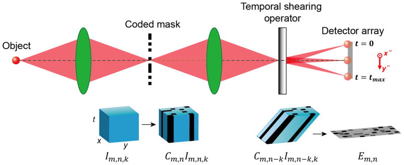
CUP image formation model. x, y, spatial coordinates; t, time; m, n, k, matrix indices; I_m,n,k, input dynamic scene element; C_m,n, coded mask matrix element; C_m,n−kI_m,n−k,k, encoded and sheared scene element; E_m,n, image element energy measured by a 2D detector array; t_max, maximum recording time.

Extended Data Fig. 2.

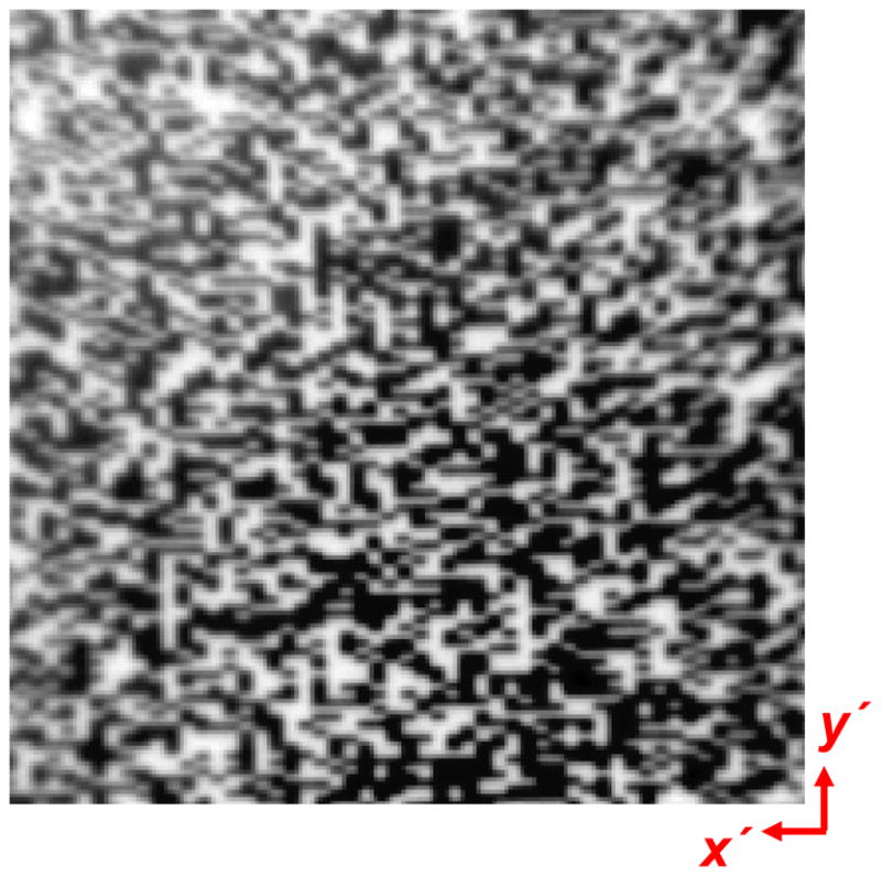
A temporally undispersed CCD image of the mask, which encodes the uniformly illuminated field with a pseudo-random binary pattern.

Extended Data Fig. 3.

Multicolour CUP. a. Custom-built spectral separation unit. b. Representative temporal frames of a pulsed-laser-pumped fluorescence emission process. The pulsed pump laser and fluorescence emission are pseudo-coloured based on their peak emission wavelengths. To explicitly indicate the spatiotemporal pattern of this event, the CUP-reconstructed frames are overlaid with a static background image captured by a monochromatic CCD camera. All temporal frames of this event are provided in Supplementary Video 6. c. Time-lapse pump laser and fluorescence emission intensities averaged within the dashed box in b. The temporal responses of pump laser excitation and fluorescence decay are fitted to a Gaussian function and an exponential function, respectively. The recovered fluorescence lifetime of Rhodamine 6G is 3.8 ns. d. Event function describing the pulsed laser fluorescence excitation. e. Event function describing the fluorescence emission. f. Measured temporal PSF, with a full width at half maximum of ~80 ps. Due to reconstruction artefacts, the PSF has a side lobe and a shoulder extending over a range of 280 ps. g. Simulated temporal responses of these two event functions after being convolved with the temporal PSF. The maxima of these two time-lapse signals are stretched by 200 ps. Scale bar, 10 mm.

References

- 1.Fuller PWW. An introduction to high speed photography and photonics. Imaging Sci J. 2009;57:293–302. doi: 10.1179/136821909x12490326247524. [DOI] [Google Scholar]
- 2.Li Z, Zgadzaj R, Wang X, Chang Y-Y, Downer MC. Single-shot tomographic movies of evolving light-velocity objects. Nat Commun. 2014;5 doi: 10.1038/ncomms4085. [DOI] [PMC free article] [PubMed] [Google Scholar]
- 3.Nakagawa K, et al. Sequentially timed all-optical mapping photography (STAMP) Nat Photon. 2014;8:695–700. doi: 10.1038/nphoton.2014.163. [DOI] [Google Scholar]
- 4.Heshmat B, Satat G, Barsi C, Raskar R. Single-shot ultrafast imaging using parallax-free alignment with a tilted lenslet array. CLEO: Science and Innovations, STu3E. 2014;7 [Google Scholar]
- 5.A Horse’s Motion Scientifically Determined. Scientific American. 1878;39:241. [Google Scholar]
- 6.Mach E, Salcher P. Photographische Fixirung der durch Projectile in der Luft eingeleiteten Vorgänge. Annalen der Physik. 1887;268:277–291. [Google Scholar]
- 7.Nebeker S. Rotating mirror cameras. High Speed Photogr Photon Newslett. 1983;3:31. [Google Scholar]
- 8.Kondo Y, et al. Development of “HyperVision HPV-X” High-speed Video Camera. Shimadzu Review. 2012;69:285–291. [Google Scholar]
- 9.El-Desouki M, et al. CMOS Image Sensors for High Speed Applications. Sensors-Basel. 2009;9:430–444. doi: 10.3390/S90100430. [DOI] [PMC free article] [PubMed] [Google Scholar]
- 10.Hamamatsu S. Guide to Streak Cameras. 2002 [Google Scholar]
- 11.Velten A, Lawson E, Bardagjy A, Bawendi M, Raskar R. Slow art with a trillion frames per second camera. ACM SIGGRAPH. 2011;44 [Google Scholar]
- 12.Velten A, et al. Recovering three-dimensional shape around a corner using ultrafast time-of-flight imaging. Nat Commun. 2012;3:745. doi: 10.1038/ncomms1747. http://www.nature.com/ncomms/journal/v3/n3/suppinfo/ncomms1747_S1.html. [DOI] [PubMed] [Google Scholar]
- 13.Solli DR, Ropers C, Koonath P, Jalali B. Optical rogue waves. Nature. 2007;450:1054–1057. doi: 10.1038/nature06402. [DOI] [PubMed] [Google Scholar]
- 14.Eldar YC, Kutyniok G. Compressed sensing: theory and applications. Cambridge University Press; 2012. [Google Scholar]
- 15.Figueiredo MAT, Nowak RD, Wright SJ. Gradient Projection for Sparse Reconstruction: Application to Compressed Sensing and Other Inverse Problems. Ieee J-Stsp. 2007;1:586–597. doi: 10.1109/Jstsp.2007.910281. [DOI] [Google Scholar]
- 16.Bioucas-Dias JM, Figueiredo MAT. A new TwIST: Two-step iterative shrinkage/thresholding algorithms for image restoration. Ieee T Image Process. 2007;16:2992–3004. doi: 10.1109/Tip.2007.909319. [DOI] [PubMed] [Google Scholar]
- 17.Afonso MV, Bioucas-Dias JM, Figueiredo MAT. Fast Image Recovery Using Variable Splitting and Constrained Optimization. Ieee T Image Process. 2010;19:2345–2356. doi: 10.1109/Tip.2010.2047910. [DOI] [PubMed] [Google Scholar]
- 18.Wright SJ, Nowak RD, Figueiredo MAT. Sparse Reconstruction by Separable Approximation. Ieee T Signal Proces. 2009;57:2479–2493. doi: 10.1109/Tsp.2009.2016892. [DOI] [Google Scholar]
- 19.Afonso MV, Bioucas-Dias JM, Figueiredo MAT. An Augmented Lagrangian Approach to the Constrained Optimization Formulation of Imaging Inverse Problems. Ieee T Image Process. 2011;20:681–695. doi: 10.1109/Tip.2010.2076294. [DOI] [PubMed] [Google Scholar]
- 20.Einstein A. Relativity: The special and general theory. Penguin; 1920. [Google Scholar]
- 21.Agrawal S, Vishwanath S. Secrecy using compressive sensing. Information Theory Workshop (ITW), 2011 IEEE. 2011:563–567. doi: 10.1109/itw.2011.6089519. [DOI] [Google Scholar]
- 22.Orsdemir A, Altun HO, Sharma G, Bocko MF. On the security and robustness of encryption via compressed sensing. Military Communications Conference, 2008. MILCOM 2008. IEEE. 2008:1–7. doi: 10.1109/milcom.2008.4753187. [DOI] [Google Scholar]
- 23.Davis DL. Secure compressed imaging. 5,907,619. US patent. 1999:25.
- 24.Borst JW, Visser AJWG. Fluorescence lifetime imaging microscopy in life sciences. Meas Sci Technol. 2010;21:102002. [Google Scholar]
Associated Data
This section collects any data citations, data availability statements, or supplementary materials included in this article.