Similarity of markers identified from cancer gene expression studies: observations from GEO

Abstract

Gene expression profiling has been extensively conducted in cancer research. The analysis of multiple independent cancer gene expression datasets may provide additional information and complement single-dataset analysis. In this study, we conduct multi-dataset analysis and are interested in evaluating the similarity of cancer-associated genes identified from different datasets. The first objective of this study is to briefly review some statistical methods that can be used for such evaluation. Both marginal analysis and joint analysis methods are reviewed. The second objective is to apply those methods to 26 Gene Expression Omnibus (GEO) datasets on five types of cancers. Our analysis suggests that for the same cancer, the marker identification results may vary significantly across datasets, and different datasets share few common genes. In addition, datasets on different cancers share few common genes. The shared genetic basis of datasets on the same or different cancers, which has been suggested in the literature, is not observed in the analysis of GEO data.

INTRODUCTION

Cancer is a disease of the genome. Gene expression profiling can measure mRNA levels and has fundamentally changed the paradigm of cancer research. Although it is one of the relatively old techniques, it is still routinely used in cancer research nowadays, partly because of the maturity of this technique and partly because of the direct connection between mRNAs and proteins. In most existing studies, a single dataset has been analyzed. In this study, we consider the analysis of multiple cancer gene expression datasets. Our main interest is in the selection of cancer-associated markers. Multi-dataset gene expression studies have been conducted in the literature. Such studies may serve the following purposes. First, consider the scenario where the same cancer outcome/phenotype has been measured in multiple datasets. Examples include [1, 2] and many others. In cancer gene expression studies, the sample sizes are usually small, which may lead to unsatisfactory data analysis results, such as low reproducibility of identified markers. Multi-dataset analysis can provide an effective way to increase sample size and hence improve analysis results. The similarity (in terms of cancer-associated markers) across multiple datasets is the basis of such analysis. Second, consider the scenario where multiple datasets measure outcomes/phenotypes on different cancers or different subtypes of the same cancer. Examples may include [3, 4] and many others. Despite great heterogeneity, cancers can be ‘similar’ or ‘interconnected’. For example, it has been shown that breast cancer and ovarian cancer share multiple susceptibility genes, including BRCA1, BRCA2 and HER2. In addition, cell cycle, apoptosis and DNA repair genes are involved in the development and progression of multiple cancers. More specific examples are provided in [4] and references therein. Comparing the susceptibility genes may facilitate the investigation of similarity and dissimilarity among different cancers and downstream analysis, such as the construction of human disease network [5].

Multi-dataset analysis includes meta-analysis and integrative analysis [2, 6]. In classic meta-analysis, multiple datasets are analyzed separately, and then summary statistics, such as the lists of identified genes, P-values and effective sizes, are pooled across datasets. In integrative analysis, the raw data of multiple datasets are analyzed simultaneously. In several recent studies [1, 2, 4], it has been argued that integrative analysis may be more informative. However, as integrative analysis methods are not as mature and well-accepted, in this study we focus on meta-analysis.

In this study, we consider the meta-analysis of multiple cancer gene expression datasets. It is noted that the reviewed techniques and empirical observations may also be applicable to other types of genetic, genomic, epigenetic and proteomic measurements. Because of limitations on data availability, we focus on etiology studies comparing cancer and normal samples and investigating the risk of cancers. The analysis of etiology studies may have multiple objectives. Here we focus on the identification of cancer-associated markers. In particular, this study has two main objectives. The first is to provide a brief review of some statistical methods that can be used to quantify the similarity of the sets of cancer markers (genetic basis) of multiple datasets. Here both marginal and joint analysis methods are discussed. The second objective is to apply these methods and conduct analysis of cancer gene expression datasets downloaded from Gene Expression Omnibus (GEO) [7]. Besides serving as the test bed of the reviewed methods, this data analysis may also serve the following important purposes. First, in the literature, multiple studies (such as [1]) have conducted meta-analysis or integrative analysis of multiple cancer gene expression datasets that measure the same outcome/phenotype, under the assumption that the genetic basis of these datasets is the same. Our analysis will provide insights into whether such an assumption is likely to be true. Second, some epidemiologic and genetic studies have suggested that certain cancers, for example, breast cancer and ovarian cancer, are ‘related’ by sharing common susceptibility genes [4]. Our analysis can show whether such similarity can be observed in the analysis of GEO gene expression datasets.

METHODS

Consider the meta-analysis of M independent datasets. With a slight abuse of notation, in a single dataset, denote as the binary cancer status, for example, presence or absence of cancer. Denote X as the length-d vector of gene expressions. Assume n iid observations . Denote as the jth component of . Many other factors, such as clinical risk factors and environmental exposures, may also contribute to cancer development. With GEO data, such variables are not available, and we focus on analyzing gene expressions. When needed, adjusting for clinical and environmental risk factors can follow the methods developed in [8] and references therein. As described in [9], in individual marker-based analysis of gene expression data, where genes are the functional units, there are two main analysis paradigms. The first is to analyze each gene separately (that is, the analysis of marginal effects) and then compare across genes. The second is to simultaneously analyze the effects of all genes (joint effects) in a single model.

Analysis of marginal effects

For gene , assume the logistic regression model, where . Here is the intercept, and is the regression coefficient. With n iid observations, the likelihood function and maximum likelihood estimate (MLE) can be obtained. Denote as the MLE of and as its P-value. With the d estimates and P-values, the similarity of genetic basis (sets of identified cancer markers) of multiple datasets can be evaluated as follows.

• [Approach 1] For each dataset, we first rank the d P-values from the smallest to the largest. The top ranked, for example, top 100 as in our numerical study, is selected. We then examine the overlap of top-ranked genes across datasets. Under Approach 1, we also consider two alternative ranking statistics. The first is the fold change, which is closely related to the difference of mean under the log scale [10]. This approach accordingly is termed as [Approach 1-fold]. The second ranking statistic is the P-value from the two-sample t-test, and this approach is termed as [Approach 1 t-test].

• [Approach 2] With the first approach, it is reinforced that all datasets identify the same number of genes. However, it is possible that in a dataset even the gene with the smallest P-value is not important. To tackle this problem, consider the false discovery rate (FDR) approach [11]. Denote α as the target FDR. The Benjamini–Hochberg threshold is defined as , where { (} are the ordered P-values (from the smallest to the largest). Genes with P-values smaller than are identified as important. We apply this approach to each dataset and then examine the overlaps of important genes across datasets. In our numerical study, we consider two target FDR values, 0.1 and 0.01. As an alternative, we also consider [Approach 2 t-test], where for each gene the P-value is from a two-sample t-test.

• [Approach 3] A limitation of the above two approaches is that they only examine whether a gene is identified in multiple datasets. The signs of the effects are not accounted for. A gene can be positively associated with response in one dataset but negatively associated in another. To overcome this limitation, we consider the genetic variation score (GVS) approach [12]. In a specific dataset, for gene , its GVS score is defined as . Thus, it combines the P-value (actual value as opposed to a simple rank), which represents the strength of association, and the sign of the estimated regression coefficient, which measures the ‘direction’ of association. For each dataset, the genetic variation profile (GVP) based on GVS is defined as , which is a vector of length d. With multiple datasets, the correlations between the GVPs can be computed, quantifying the similarity of gene effects. Here we consider three different correlations, namely, Pearson, Kendall and Spearman. The last two correlations are based on rank and can be more robust. Once correlations are computed, hierarchical clustering of datasets can be conducted using the flashclust function in R. The clustering results can reveal whether two datasets have similar genetic profiles.

In the above analysis, the logistic regression model is adopted, which is the default for data with binary responses. In the recent literature, model-free approaches have been developed [8]. Although they may possess the robustness property, they suffer from high computational cost and lack of stability and have not been extensively adopted. There are many other ways of quantifying similarity. For example, multiple statistics have been described in [10] for ranking genes. Here we mostly focus on P-value-based approaches because of their popularity.

Analysis of joint effects

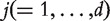
As an alternative to marginal analysis, joint analysis simultaneously accounts for the effects of all genes. For subject i in a specific dataset, still assume the logistic model , where is the intercept, and is the vector of regression coefficient. With gene expression data, for example, those analyzed in the next section, , and MLE cannot be straightforwardly computed. In addition, it is expected that of a large number of profiled genes, only a small subset is associated with the response. With such considerations, we consider the Lasso penalized estimate [13, 14], which is defined as:

is the data-dependent tuning parameter, and is selected using V-fold cross validation in data analysis. is the jth component of . Genes corresponding to the non-zero components of are identified as associated with cancer [13]. After Lasso estimation and gene selection are applied to each dataset, we can evaluate the overlaps of identified genes across datasets. In data analysis, Lasso is realized using R package glmnet.

The Lasso estimate (as well as other penalized estimates) and hence the set of selected genes depend on the tuning parameter. Although there have been extensive investigations, choosing the proper tuning for a practical dataset still remains a challenging problem. To partly overcome the tuning selection problem, the stability selection approach [15] has been suggested and proceeds as follows. For each dataset (a) randomly select half of the observations without replacement. Apply Lasso estimation; (b) repeat Step (a) 100 times; (c) for each gene, compute its probability of being selected in the 100 samplings; and (d) genes with probabilities of being selected over a certain cutoff are identified. After this procedure is applied to each dataset separately, we can evaluate the overlap of identified important genes. The cutoff parameter is user-determined. In the GEO data analysis, we find that there are few genes with high probabilities of being selected. We thus set a loose cutoff as 0.1. In the GEO data analysis, some datasets have small sample sizes, as can be seen from Table 1. With small datasets, selecting half of the subjects leads to an even smaller sample size and may create a convergence problem when computing Lasso. Thus, the stability selection approach is only applied to datasets with at least six controls.

Table 1:

Overview of the 26 GEO datasets

Type	Series no and platform	Case	Control	Reference
Breast	_GSE14548_GPL1352	38	28	[16]
Breast	_GSE14999_GPL3991	68	61	[17]
Breast	_GSE15852_GPL96	43	43	[18]
Breast	_GSE20086_GPL570	6	6	[19]
Breast	_GSE21947_GPL96	15	15	[20]
Breast	_GSE22544_GPL570	16	4	[21]
Breast	_GSE22820_GPL4133	176	10	[22]
Breast	_GSE33447_GPL14550	8	8	[23]
Breast	_GSE3744_GPL570	40	7	[24]
Breast	_GSE5364_GPL96	183	13	[25]
Breast	_GSE7882_GPL5326	54	7	[26]
Breast	_GSE9574_GPL96	14	15	[27]
Lymphoma	_GSE28442_GPL570	4	4	GEO website
Ovarian	_GSE12470_GPL887	43	10	[28]
Ovarian	_GSE14407_GPL570	12	12	[29]
Ovarian	_GSE15578_GPL570	11	6	GEO website
Ovarian	_GSE18520_GPL570	53	10	[30]
Pancreatic	_GSE16515_GPL570	36	16	[31]
Pancreatic	_GSE19650_GPL570	15	7	[32]
Prostate	_GSE11682_GPL4133	17	17	[33]
Prostate	_GSE12378_GPL5175	36	3	[34]
Prostate	_GSE14206_GPL887	53	14	[35]
Prostate	_GSE16120_GPL887	51	14	[36]
Prostate	_GSE17906_GPL570	13	12	[37]
Prostate	_GSE29079_GPL5175	47	48	[38]
Prostate	_GSE32269_GPL96	51	4	GEO website

The two Lasso-based approaches described above only examine whether a gene is selected or not. Loosely speaking, they correspond to Approaches 1 and 2 under marginal analysis. Conceptually, it is possible to develop the joint analysis counterpart of Approach 3. However, in high-dimensional analysis, there is still extensive debate on how to compute P-values. There are a few approaches with asymptotic validity. However, in practical data analysis, they are only moderately successful. To be conservative, we will not examine joint analysis approach that involves significance level. In the literature, there are a large number of studies implementing Lasso penalization to cancer gene expression data [13, 39, 40]. Many alternative approaches, such as boosting, thresholding, Bayesian, can be applied to analyze the joint effects of genes. Penalization can be preferred, as it has lucid statistical properties, affordable computational cost and satisfactory empirical performance [13, 40]. Beyond Lasso, other penalization approaches, such as bridge, minimax concave penalty and smoothly clipped absolute deviation, are also applicable. Lasso is chosen, as numerically it is the simplest and the most stable. In stability selection, the cutoff is much lower than that considered in [15]. With a higher cutoff, few or none of the genes in GEO analysis may be selected. Multiple factors may contribute to the overall low probabilities. The first, and most important, is the small sample size of individual datasets. Second, in cancer genomic studies, the signals are usually weak. In addition, as with any statistical approach, the performance of penalized methods may still need improvement.

ANALYSIS OF GEO DATA

GEO [7], or Gene Expression Omnibus, is a National Center for Biotechnology Information database for gene expression data. It hosts a large number of cancer genomic datasets. Datasets to be analyzed were assembled in June 2012. Our data collection has been limited to human cancer studies with both case and control samples using one channel microarrays. Our search identifies 28 datasets. Two of them are removed as they profiled a very small number of genes. A total of 26 datasets are included in data analysis, covering five types of cancers. There are 12 datasets on breast cancer, 1 on lymphoma, 4 on ovarian cancer, 2 on pancreatic cancer and 7 on prostate cancer. All of the datasets used total RNA extracted from human carcinoma specimens, which were clinically removed from cancer patients. Brief information on the datasets is provided in Table 1. Nine microarray platforms were used in profiling. In our analysis, we use the processed gene expression values available from the GEO depository. A total of 6890 genes are profiled in all 26 datasets. Following [12], our analysis is focused on those genes only. It is acknowledged that some important genes may be left out by this screening. However, as the number of genes left is still large, this may not be a serious concern. In addition, using all genes may create a missing measurement problem, which brings additional complexity.

Analysis of marginal effects

The analysis results of Approach 1, Approach 1-fold and Approach 1 t-test are shown in Table 2, Supplementary Tables S1 and S2, respectively. Detailed results using different ranking statistics are slightly different. However, the overall observed patterns are similar. This is in line with [10], which shows that marginal rankings using several commonly adopted statistics (including the three investigated here) are highly correlated. Take Table 2 as an example. The first observation is that for datasets on the same type of cancer, the number of overlapped genes ranked in the top 100 is small. For breast cancer, the largest number of overlap is 27; for ovarian cancer, it is 4; for pancreatic cancer, the two identified sets have 4 genes in common; and for prostate cancer, the largest number of overlap is 74. The second observation is that the sets of top 100 genes identified in datasets on different types of cancers have very small overlap. Examining the off-block-diagonal elements of Table 2 shows that the largest number of overlap is 8.

Table 2:

Marginal analysis, Approach 1: overlaps of top 100 ranked genes across the 26 datasets

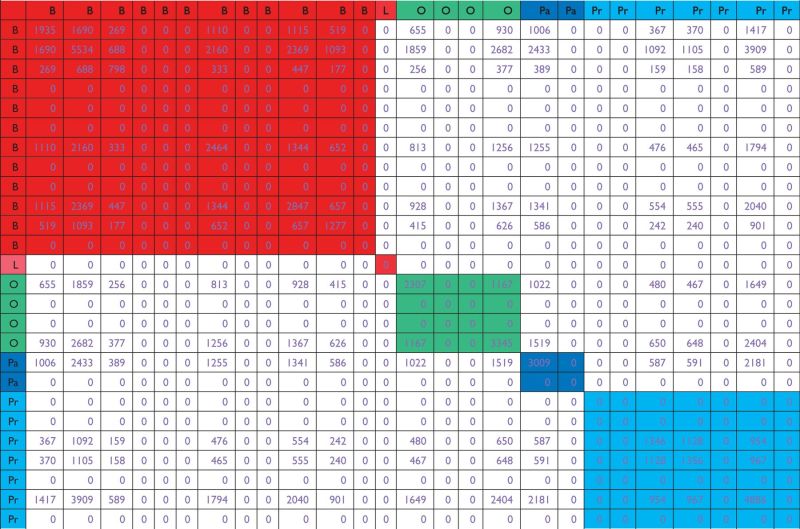
The analysis results of Approach 2 and Approach 2 t-test with FDR = 0.1 are shown in Table 3 and Supplementary Table S3, respectively. We have also examined results with FDR = 0.01. Fewer genes are identified, but the overall patterns of observations are similar. We again observe that using logistic regression and t-test leads to different numerical results but similar qualitative conclusions. Take Table 3 as an example. It shows that with the FDR control, different datasets on the same cancer may identify a dramatically different number of genes. Consider, for example, the four ovarian cancer datasets. The numbers of identified genes are 2307, 0, 0 and 3345, respectively. In some cases, there is an ‘improvement’ in overlap. Consider the first and fourth ovarian cancer datasets. Under Approach 1, the two top 100 sets have four genes in common. Under Approach 2, total of 1167 common genes are identified by the two datasets. The second observation is that for datasets on different types of cancers, there may also be ‘improvement’ in the overlap. Consider, for example, the first breast cancer and the first ovarian cancer datasets. Under Approach 1, there are two overlapped genes. As a comparison, under Approach 2, there are 655 genes in common.

Table 3:

Marginal analysis, Approach 2: overlaps of genes selected using FDR = 0.1 across the 26 datasets

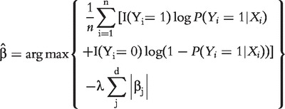
The analysis results of Approach 3 are shown in Figures 1–3 for the three correlations. The heat maps show the correlation matrices between the GVPs. Positive correlations are shown in red, and negative correlations are shown in green. Different cancers are represented using different colors shown on the left of the figures. Examining the figures shows that different correlations lead to different quantitative results,;however, the qualitative observations are similar. Consider, for example, Figure 1. Except for several breast cancer datasets, in general, the correlations among datasets on the same cancers are weak. For different types of cancers, the correlations are mostly weak. Hierarchical clustering can cluster some datasets on the same cancers together, but not always. For example with the four ovarian cancer datasets, the first level of clustering puts GSE14407 and GSE 18520 in the same cluster; GSE15578 and GSE12470 are put in the same cluster in the second level of clustering. However, the two clusters do not unite until at the last level.

Figure 1:

Analysis of marginal effects: Approach 3 with Pearson correlation.

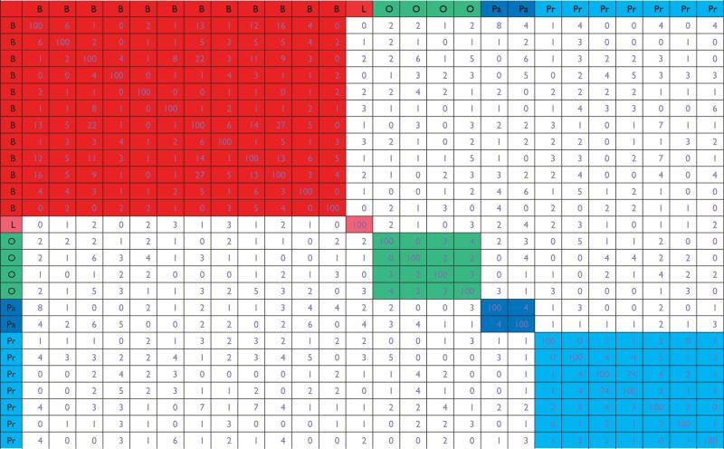
Figure 2:

Analysis of marginal effects: Approach 3 with Kendall correlation.

Figure 3:

Analysis of marginal effects: Approach 3 with Spearman correlation.

The 26 datasets use nine different platforms. It is possible that there may be batch effects, which may potentially bias the analysis. Multiple methods have been developed to correct such effects [41]. Examples may include singular value decomposition, standard linear regression, Combat, surrogate variable analysis (SVA) and others. Here we apply the Combat function in the SVA package [42], which conducts cross-platform normalization using empirical Bayes approach. Compared with other methods, Combat can be robust to outliers in small datasets. Supplementary Figures 1–3 correspond to Figures 1–3, with cross-platform normalized data. The observations are slightly different, but the overall conclusions are similar.

Analysis of joint effects

We apply the Lasso approach to each dataset separately. The tuning parameter is selected using 5-fold cross validation. Results are shown in Table 4. A small number of genes are identified as cancer-associated genes. For breast cancer, the largest number of identified genes for a single dataset is 26, and the smallest number is 0. For the lymphoma dataset, four genes are identified. For the four ovarian datasets, 6, 4, 1, and 10 genes are identified, respectively. For the two pancreatic cancer datasets, 0 and 5 genes are identified. And for the prostate cancer datasets, the largest number is 27, and the smallest number is 0. It is concluded that for the same cancers, the gene identification results can be significantly different. For datasets on different types of cancers, one gene is shared by a breast and an ovarian cancer datasets, and another gene is shared by a breast and a pancreatic cancer datasets. Otherwise, there is no common gene.

Table 4:

Analysis of joint effects: Lasso

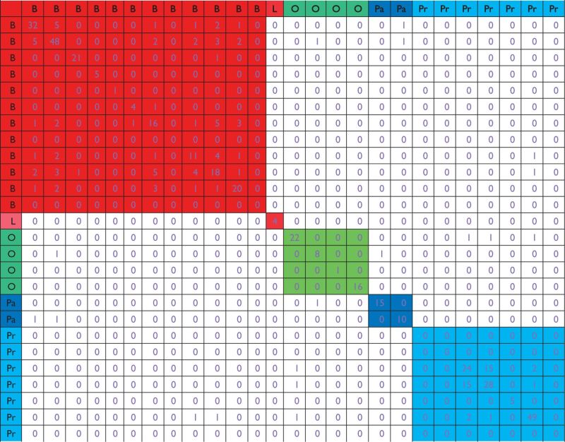
The ‘stability selection + Lasso’ approach is applied to each dataset. Results are summarized in Table 5. With a relatively loose cutoff (0.1), this approach identifies more genes than the straightforward application of Lasso. For example, for the first breast cancer dataset, 32 genes are identified, compared with 26 in Table 4. For the two pancreatic cancer datasets, 15 and 10 genes are identified, compared with 0 and 5 in Table 4. However, for datasets on the same or different cancers, the number of overlapped genes remains small.

Table 5:

Analysis of joint effects: stability selection with cutoff 0.1

DISCUSSION

In the literature, when analyzing independent datasets on the same cancers, some studies such as [1, 2] reinforce that different datasets share the same set of susceptibility genes. It should be noted that the validity of such a condition has not been carefully checked. In our analysis of marginal and joint effects, we observe that the number of overlapped genes is small. In the analysis of datasets on different types of cancers, several studies including [4, 43, 44] have suggested that multiple cancers share common markers. A few pathways, such as DNA repair, cell cycle, apoptosis and RAS, have been generally suggested as ‘cancer associated’. However, in our analysis, it is observed that even though multiple cancers may have overlapped markers, the degree of overlap is small.

Multiple factors may have contributed to the discrepancy between our analysis results and the published ones. First, data quality may plan an important role. Multi-dataset analysis results hinge on the quality of each individual dataset. Our data selection has been conducted in an ‘unsupervised’ manner. Without having access to original experimental details and raw data, quality control has not been conducted. It is known that the quality of GEO datasets varies. GEO is selected, as it contains a large number of public datasets and has been used in many studies. Analysis of more controlled datasets, such as TCGA (The Cancer Genome Atlas), may potentially lead to different conclusions. Second, the analysis strategies have been different. In this study, we first identify the ‘strongest signals’ for each individual dataset, and then search for overlaps across datasets. In studies such as [43], the strategy is to search for genes showing persistent effects across cancer types (while genes showing strong effects in one or a small number of datasets are not of interest). Note that such genes do not necessarily have the strongest effects for each individual cancer. Third, in cancer gene expression studies, it is commonly agreed that the signals are in general weak, even for those well-known ‘cancer genes’. This, coupled with the high variability of gene expression measurements, may create high variation in gene identification. Fourth, several aspects of our analysis still need improvement. Normalization plays an important role in microarray analysis. In our analysis, each dataset has been processed separately. In addition, we have experimented cross-platform normalization using Combat. Nevertheless, without having access to the raw data, there may be ‘residual’ batch effects to bias the analysis. In our analysis, genes are the functional units. It has been suggested that pathway-based analysis may increase stability and partly solve the lack-of-overlapped gene problem [45]. A large number of analyses conducted nowadays are still gene-based. In addition, many genes in the GEO datasets are not well curated. Thus, here we have focused on gene-based analysis. It should be noted that with our analysis (and many of similar kind in the literature), only associations between genes and cancer risk can be established. More definitive results on causation demand more profiling data and finer mechanistic studies.

CONCLUSION

Although in the literature single-dataset analysis still dominates, recent studies have suggested that multi-datasets analysis may provide additional insights and complement single-dataset analysis. In this study, we have focused on the similarity of genes identified in multiple cancer gene expression studies, which is an important aspect of multi-datasets analysis. A few existing statistical methods are reviewed. It is noted that there are other methods that can serve similar purposes. For example, the logistic-model-based methods can be replaced with those based on other generalized linear models. In addition, there are many others methods that can analyze the joint effects of all genes. The similarity of identified gene sets is evaluated using the number of overlapped genes, whereas measures such as the Jaccard index can be more comprehensive. Here it is noted that as the degree of overlap is really small, we do not expect significantly different results with other overlap measures. The reviewed methods are relatively simple and more extensively adopted, and hence deserve higher priority.

Twenty-six GEO datasets are analyzed, and few overlapped genes are identified. It is noted that our analysis does not rule out the possibility that datasets on the same or different cancers share common genes. It is simply that such shared genes are not commonly observed using the reviewed methods and GEO microarray datasets. In the above section, we enumerate multiple possible reasons why our findings are different from the published studies. Identifying the exact cause is of great interest. However, it does not seem feasible without having access to all the experimental details and conducting mechanistic studies.

SUPPLEMENTARY DATA

Supplementary data are available online at http://bib.oxfordjournals.org/.

Key Points.

• Multi-dataset analysis may provide additional insights beyond single-dataset analysis in cancer gene expression profiling studies.

• There are statistical methods that can be used to evaluate the similarity of identified genes in multi-dataset analysis. Both marginal and joint effects can be analyzed.

• In the analysis of GEO datasets, it is found that different datasets on the same cancers may lead to significantly different gene identification results. Few genes are identified in multiple datasets.

• In the analysis of GEO datasets, it is found that there are few genes shared by datasets on different types of cancers.

Biographies

Xingjie Shi is a doctoral student in statistics/biostatistics currently under a joint training program by the Shanghai University of Finance and Economics and Yale University.

Shihao Shen obtained his Ph.D. in Biostatistics from the University of Iowa. He is now a Postdoctoral Associate at the University of California, Los Angeles.

Jin Liu obtained his Ph.D. in Statistics from the University of Iowa. He is now a Postdoctoral Associate at the Department of Biostatistics, Yale University.

Jian Huang obtained his Ph.D. in Statistics from the University of Washington. He is Professor of Statistics at the University of Iowa.

Yong Zhou is Professor and Associate Dean at the School of Statistics, Shanghai University of Finance and Economics.

Shuangge Ma obtained his Ph.D. in Statistics from the University of Wisconsin, Madison. He is Associate Professor of Biostatistics at Yale University.

FUNDING

This study was supported by awards CA142774, CA165923 and CA152301 from National Institute of Health, DMS1208225 from National Science Foundation, a Pilot Grant from the Yale Comprehensive Cancer Center and 2012LD001 from National Bureau of Statistics of China.

References

- 1.Ma S, Huang J, Wei F, et al. Integrative analysis of multiple cancer prognosis studies with gene expression measurements. Stat Med. 2011;30:3361–71. doi: 10.1002/sim.4337. [DOI] [PMC free article] [PubMed] [Google Scholar]
- 2.Huang Y, Huang J, Shia BC, et al. Identification of cancer genomic markers via integrative sparse boosting. Biostatistics. 2012;13:509–22. doi: 10.1093/biostatistics/kxr033. [DOI] [PMC free article] [PubMed] [Google Scholar]
- 3.Ma S, Zhang Y, Huang J, et al. Integrative analysis of cancer prognosis data with multiple subtypes using regularized gradient descent. Genet Epidemiol. 2012;36:829–38. doi: 10.1002/gepi.21669. [DOI] [PMC free article] [PubMed] [Google Scholar]
- 4.Ma S, Huang J, Moran M. Identification of genes associated with multiple cancers via integrative analysis. BMC Genomics. 2009;10:535. doi: 10.1186/1471-2164-10-535. [DOI] [PMC free article] [PubMed] [Google Scholar]
- 5.Goh KI, Choi IG. Exploring the human diseasome: the human disease network. Brief Funct Genomics. 2012;11:533–42. doi: 10.1093/bfgp/els032. [DOI] [PubMed] [Google Scholar]
- 6.Guerra R, Goldstein DR. Meta-analysis and Combining Information in Genetics and Genomics. Chapman & Hall/CRC; 2009. [Google Scholar]
- 7.Gene Expression Omnibus. http://www.ncbi.nlm.nih.gov/geo/ (15 April 2013, date last accessed)
- 8.Yu T, Li J, Ma S. Adjusting confounders in ranking biomarkers: a model-based ROC approach. Brief Bioinform. 2012;13:513–23. doi: 10.1093/bib/bbs008. [DOI] [PMC free article] [PubMed] [Google Scholar]
- 9.Witten DM, Tibshirani R. Survival analysis with high-dimensional covariates. Stat Methods Med Res. 2010;19:29–51. doi: 10.1177/0962280209105024. [DOI] [PMC free article] [PubMed] [Google Scholar]
- 10.Ma S. Empirical study of supervised gene screening. BMC Bioinformatics. 2006;7:537. doi: 10.1186/1471-2105-7-537. [DOI] [PMC free article] [PubMed] [Google Scholar]
- 11.Bhattacharjee M, Dhar SK, Subramanian S. Recent Advances in Biostatistics: False Discovery Rates, Survival Analysis, and Related Topics. World Scientific Publishing Company; 2011. [Google Scholar]
- 12.Sirota M, Schaub MA, Batzoglous S, et al. Autoimmune disease classification by inverse association with SNP alleles. PLoS Genet. 2009;5:e1000792. doi: 10.1371/journal.pgen.1000792. [DOI] [PMC free article] [PubMed] [Google Scholar]
- 13.Ma S, Huang J. Penalized feature selection and classification in bioinformatics. Brief Bioinform. 2008;9:392–403. doi: 10.1093/bib/bbn027. [DOI] [PMC free article] [PubMed] [Google Scholar]
- 14.Huang J, Breheny P, Ma S. A selective review of group selection in high dimensional models. Stat Sci. 2012;27:481–99. doi: 10.1214/12-STS392. [DOI] [PMC free article] [PubMed] [Google Scholar]
- 15.Meinshausen N, Buhlmann P. Statbility selection. J R Stat Soc Series B Stat Methodol. 2010;72:417–73. [Google Scholar]
- 16.Ma XJ, Dahiya S, Richardson E, et al. Gene expression profiling of the tumor microenvironment during breast cancer progression. Breast Cancer Res. 2009;11(1):R7. doi: 10.1186/bcr2222. [DOI] [PMC free article] [PubMed] [Google Scholar]
- 17.Uva P, Aurisicchio L, Watters J, et al. Comparative expression pathway analysis of human and canine mammary tumors. BMC Genomics. 2009;10:135. doi: 10.1186/1471-2164-10-135. [DOI] [PMC free article] [PubMed] [Google Scholar]
- 18.Pau Ni IB, Zakaria Z, Muhammad R, et al. Gene expression patterns distinguish breast carcinomas from normal breast tissues: the Malaysian context. Pathol Res Pract. 2010;206(4):223–8. doi: 10.1016/j.prp.2009.11.006. [DOI] [PubMed] [Google Scholar]
- 19.Bauer M, Su G, Casper C, et al. Heterogeneity of gene expression in stromal fibroblasts of human breast carcinomas and normal breast. Oncogene. 2010;29(12):1732–40. doi: 10.1038/onc.2009.463. [DOI] [PMC free article] [PubMed] [Google Scholar]
- 20.Graham K, Ge X, de Las Morenas A, et al. Gene expression profiles of estrogen receptor-positive and estrogen receptor-negative breast cancers are detectable in histologically normal breast epithelium. Clin Cancer Res. 2011;17(2):236–46. doi: 10.1158/1078-0432.CCR-10-1369. [DOI] [PMC free article] [PubMed] [Google Scholar]
- 21.Hawthorn L, Luce J, Stein L, et al. Integration of transcript expression, copy number and LOH analysis of infiltrating ductal carcinoma of the breast. BMC Cancer. 2010;10:460. doi: 10.1186/1471-2407-10-460. [DOI] [PMC free article] [PubMed] [Google Scholar]
- 22.Liu RZ, Graham K, Glubrecht DD, et al. Association of FABP5 expression with poor survival in triple-negative breast cancer: implication for retinoic acid therapy. Am J Pathol. 2011;178(3):997–1008. doi: 10.1016/j.ajpath.2010.11.075. [DOI] [PMC free article] [PubMed] [Google Scholar]
- 23.Lian ZQ, Wang Q, Li WP, et al. Screening of significantly hypermethylated genes in breast cancer using microarray-based methylated-CpG island recovery assay and identification of their expression levels. Int J Oncol. 2012;41(2):629–38. doi: 10.3892/ijo.2012.1464. [DOI] [PubMed] [Google Scholar]
- 24.Richardson AL, Wang ZC, De Nicolo A, et al. X chromosomal abnormalities in basal-like human breast cancer. Cancer Cell. 2006;9(2):121–32. doi: 10.1016/j.ccr.2006.01.013. [DOI] [PubMed] [Google Scholar]
- 25.Yu K, Ganesan K, Tan LK, et al. A precisely regulated gene expression cassette potently modulates metastasis and survival in multiple solid cancers. PLoS Genet. 2008;4(7):e1000129. doi: 10.1371/journal.pgen.1000129. [DOI] [PMC free article] [PubMed] [Google Scholar]
- 26.Balleine RL, Webster LR, Davis S, et al. Molecular grading of ductal carcinoma in situ of the breast. Clin Cancer Res. 2008;14(24):8244–52. doi: 10.1158/1078-0432.CCR-08-0939. [DOI] [PMC free article] [PubMed] [Google Scholar]
- 27.Tripathi A, King C, de la Morenas A, et al. Gene expression abnormalities in histologically normal breast epithelium of breast cancer patients. Int J Cancer. 2008;122(7):1557–66. doi: 10.1002/ijc.23267. [DOI] [PubMed] [Google Scholar]
- 28.Yoshihara K, Tajima A, Komata D, et al. Gene expression profiling of advanced-stage serous ovarian cancers distinguishes novel subclasses and implicates ZEB2 in tumor progression and prognosis. Cancer Sci. 2009;100(8):1421–8. doi: 10.1111/j.1349-7006.2009.01204.x. [DOI] [PMC free article] [PubMed] [Google Scholar]
- 29.Bowen NJ, Walker LD, Matyunina LV, et al. Gene expression profiling supports the hypothesis that human ovarian surface epithelia are multipotent and capable of serving as ovarian cancer initiating cells. BMC Med Genomics. 2009;2:71. doi: 10.1186/1755-8794-2-71. [DOI] [PMC free article] [PubMed] [Google Scholar]
- 30.Mok SC, Bonome T, Vathipadiekal V, et al. A gene signature predictive for outcome in advanced ovarian cancer identifies a survival factor: microfibril-associated glycoprotein 2. Cancer Cell. 2009;16(6):521–32. doi: 10.1016/j.ccr.2009.10.018. [DOI] [PMC free article] [PubMed] [Google Scholar]
- 31.Pei H, Li L, Fridley BL, et al. FKBP51 affects cancer cell response to chemotherapy by negatively regulating Akt. Cancer Cell. 2009;16(3):259–66. doi: 10.1016/j.ccr.2009.07.016. [DOI] [PMC free article] [PubMed] [Google Scholar]
- 32.Hiraoka N, Yamazaki-Itoh R, Ino Y, et al. CXCL17 and ICAM2 are associated with a potential anti-tumor immune response in early intraepithelial stages of human pancreatic carcinogenesis. Gastroenterology. 2011;140(1):310–21. doi: 10.1053/j.gastro.2010.10.009. [DOI] [PubMed] [Google Scholar]
- 33.Dakhova O, Ozen M, Creighton CJ, et al. Global gene expression analysis of reactive stroma in prostate cancer. Clin Cancer Res. 2009;15(12):3979–89. doi: 10.1158/1078-0432.CCR-08-1899. [DOI] [PMC free article] [PubMed] [Google Scholar]
- 34.Jhavar S, Brewer D, Edwards S, et al. Integration of ERG gene mapping and gene-expression profiling identifies distinct categories of human prostate cancer. BJU Int. 2009;103(9):1256–69. doi: 10.1111/j.1464-410X.2008.08200.x. [DOI] [PubMed] [Google Scholar]
- 35.Kunderfranco P, Mello-Grand M, Cangemi R, et al. ETS transcription factors control transcription of EZH2 and epigenetic silencing of the tumor suppressor gene Nkx3.1 in prostate cancer. PLoS One. 2010;5(5):e10547. doi: 10.1371/journal.pone.0010547. [DOI] [PMC free article] [PubMed] [Google Scholar]
- 36.Peraldo-Neia C, Migliardi G, Mello-Grand M, et al. Epidermal Growth Factor Receptor (EGFR) mutation analysis, gene expression profiling and EGFR protein expression in primary prostate cancer. BMC Cancer. 2011;11:31. doi: 10.1186/1471-2407-11-31. [DOI] [PMC free article] [PubMed] [Google Scholar]
- 37.Pascal LE, Goo YA, Vêncio RZ, et al. Gene expression down-regulation in CD90+ prostate tumor-associated stromal cells involves potential organ-specific genes. BMC Cancer. 2009;9:317. doi: 10.1186/1471-2407-9-317. [DOI] [PMC free article] [PubMed] [Google Scholar]
- 38.Brase JC, Johannes M, Mannsperger H, et al. TMPRSS2-ERG -specific transcriptional modulation is associated with prostate cancer biomarkers and TGF-β signaling. BMC Cancer. 2011;11:507. doi: 10.1186/1471-2407-11-507. [DOI] [PMC free article] [PubMed] [Google Scholar]
- 39.Ma S, Song X, Huang J. Supervised group Lasso with applications to microarray data analysis. BMC Bioinformatics. 2007;8:60. doi: 10.1186/1471-2105-8-60. [DOI] [PMC free article] [PubMed] [Google Scholar]
- 40.Huang J, Ma S, Zhang C. Adaptive Lasso for sparse high dimensional regression models. Stat Sin. 2008;18:1603–18. [Google Scholar]
- 41.Stafford P. Methods in Microarray Normalization. CRC Press; 2008. [Google Scholar]
- 42.Surrogate Variable Analysis. http://www.bioconductor.org/packages/2.11/bioc/html/sva.html (15 April 2013, date last accessed)
- 43.Rhodes DR, Yu J, Shanker K, et al. Large-scale meta-analysis of cancer microarray data identifies common transcriptional profiles of neoplastic transformation and progression. Proc Natl Acad Sci USA. 2004;25:9309–14. doi: 10.1073/pnas.0401994101. [DOI] [PMC free article] [PubMed] [Google Scholar]
- 44.Xu L, Geman D, Winslow RL. Large-scale integrative of cancer microarray data identifies a robust common cancer signature. BMC Bioinformatics. 2007;8:275. doi: 10.1186/1471-2105-8-275. [DOI] [PMC free article] [PubMed] [Google Scholar]
- 45.Knudsen S. Cancer Diagnostics with DNA Microarrays. Wiley-Liss; 2006. [Google Scholar]
Associated Data
This section collects any data citations, data availability statements, or supplementary materials included in this article.