The dilemma of choosing the ideal permutation strategy while estimating statistical significance of genome-wide enrichment

Abstract

Integrative analyses of genomic, epigenomic and transcriptomic features for human and various model organisms have revealed that many such features are nonrandomly distributed in the genome. Significant enrichment (or depletion) of genomic features is anticipated to be biologically important. Detection of genomic regions having enrichment of certain features and estimation of corresponding statistical significance rely on the expected null distribution generated by a permutation model. We discuss different genome-wide permutation approaches, present examples where the permutation strategy affects the null model and show that the confidence in estimating statistical significance of genome-wide enrichment might depend on the choice of the permutation approach. In those cases, where biologically relevant constraints are unclear, it is preferable to examine whether key conclusions are consistent, irrespective of the choice of the randomization strategy.

INTRODUCTION

Recent advances in high-throughput genomic technologies have allowed rapid production of genome-wide genomic, epigenomic and transcriptomic data for human and various model organisms [1]. Integrative analyses using these high-throughput data sets have revealed that many genomic, epigenomic and evolutionary features are nonrandomly distributed in the genome, and hypothesized that such enrichment might be biologically relevant [2]. Local enrichment of genomic and epigenomic features has led to discoveries of novel functional elements and uncovered new design principles of the genome [2, 3]. One classic example is the genome-wide discovery of long noncoding RNAs, which were identified based on histone modification signatures and multispecies evolutionary conservation [4]. Similar methods were used to identify co-occurrence and spatial arrangement of transcription factor binding motifs and frequent combinations of histone modifications, which opened up new paradigms of combinatorial regulations [5–7]. Recently, as a part of the ENCODE initiative, in an analysis combining ChIPseq data for 100 transcription factors from multiple cell types, three pairs of regulatory regions were identified: (i) regions with active or inactive transcription factor binding, (ii) regions with high or low degrees of cobinding (termed HOT and LOT regions) and (iii) regulatory modules proximal or distal to genes. The latter were used to identify potential enhancers, which were then validated experimentally [8]. Integrative analyses of cancer genomic data sets helped demonstrate that genomic regions enriched in somatic amplifications and deletions contain key cancer-associated genes [9], and that the end points of these amplifications and deletions frequently overlap with G-quadruplex motifs (guanine-rich sequences that can form a four-stranded structure) [10], and also have characteristic DNA replication timing patterns [11]. Another example is single-cell sequencing, where local enrichment patterns of sequence read coverage were used to infer amplifications and deletions [12, 13].

In most of the above examples, statistical significance of nonrandom distribution of genomic and epigenomic features relies on the expected null distribution, typically generated using a permutation model. Is there an ideal permutation strategy in any given scenario? If not, how do the permutation assumptions affect statistical significance? In that case, which permutation strategy should we use while estimating statistical significance of genome-wide enrichment of a given feature? Later in the text, we discuss the common metrics for determining likelihood of observed data, different types of permutation strategies adopted by published studies, the software available for different types of genome-wide permutation (or shuffling) and the dilemma of choosing the ideal permutation strategy for generating an appropriate null model. Although some of the previous reviews focused on more specialized topics (e.g. transcription factor colocalization) [14], we aim to provide a more general overview on the dilemma of choosing the ‘ideal’ null model. Then, using two case studies, we highlight the consequences of different permutation assumptions, and the dilemma it may pose while interpreting the results for specific applications. We conclude by recommending that when biologically relevant constraints are unclear, it is preferable to highlight the assumptions of the null model and also examine whether key conclusions are consistent, irrespective of the choice of the null model. As such, the behavior under a variety of null models can provide insight into the distribution of the observed data.

METRIC FOR DETERMINING LIKELIHOOD OF OBSERVED DATA

At the very basis of a permutation strategy is the metric for determining likelihood of observed data. In most cases, the simplest estimated parameters are either the total base pairs of overlap, or the number of overlapping features between two data sets. Fu and Adryan [14] have enumerated a number of other metrics for comparing observed and expected patterns. For example, one can create a contingency table for occupancy of the intervals from one set, the intervals from another or both, which can then be the basis for the chi-square test or the hypergeometric before any shuffling is performed. Fu and Adryan have also listed the practice of combining P-values from bins, which could be extended for use in permutations by comparing the number of co-occurrences in each bin. Another single metric for defining the overlap is the Jaccard index—defined as the total length of overlap divided by the sum of the lengths of the union of all intervals. Other metrics may include sum of distances to the k-nearest intervals, number of complete overlaps (excluding partial overlaps) or the number of co-occurrences in some predefined bins. For instance, to determine significance of pairwise co-occurrences of two features that show dense clustering across the genome (burstiness), Haiminen et al. calculated a co-occurrence score—the number of times occurrence of the first feature is followed or preceded by at least one event of the second feature within a predefined distance [15]. See [15, 16] for similar scores. In summary, the choice of metric will ultimately depend on the question at hand.

DIFFERENT TYPES OF PERMUTATION APPROACHES

Basic approach

A basic approach (Figure 1A) while estimating genome-wide enrichment of a genomic, epigenomic or transcriptomic feature is to first overlay that data along the genome, and calculate the observed frequency at various locations in the genome. Next, one needs to choose a permutation strategy to generate the expected null distribution, where these elements are iteratively redistributed ‘randomly’ throughout the genome. Finally, the observed frequencies are compared against the expected frequencies based on the permutations to estimate the enrichment of that feature at various genomic locations or at a genome-wide scale. The randomization can be done in several ways.

Figure 1:

(A) The basic principle behind permutation analysis to determine genome-wide enrichment of a genomic or epigenomic feature. (B) A different randomization strategy can produce a different expected distribution, and hence affect statistical significance of enrichment of the feature. In (Biii), disallowed regions are masked (gray) while shuffling with additional constraints. The displayed list does not represent the exhaustive list of possible randomization strategies. A colour version of this figure is available at BIB online: http://bib.oxfordjournals.org.

Randomization across the genome or within the chromosomes

One of the simplest permutation strategies allows placing the elements of a given feature anywhere on the genome (which could be on the same chromosome or other chromosomes) without any restriction, and allowing overlap among the randomized elements (Figure 1Bi). This permutation strategy has minimal assumptions, and is widely used.

However, in certain scenarios the simplest solution is not the best one, and a more constrained permutation approach is biologically more relevant. For instance, it is found that arm-level and whole-chromosome-level amplifications and deletions are common in cancer genomes [17], probably because of mis-segregation during mitosis. Because different chromosomes have different sizes, unconstrained shuffling of these amplifications and deletion events across the genome would generate a biologically inconsistent null distribution, leading to incorrect estimation of enrichment and statistical significance. Similarly, sex chromosomes have different copy numbers in male and female, and thus one might prefer to treat sex chromosomes separately. In these cases, one might prefer to perform the shuffling within respective chromosomes (Figure 1Bii). GISTIC [9], a widely used algorithm for identifying significant amplification and deletion events, randomizes the amplification and deletion events within respective chromosomes as default. Similarly, BEDTools [18], a common genome analysis tool, allows the user to select randomization across the genome or within respective chromosomes. In general, when the relative proportion of the elements of the given feature differs considerably between the chromosomes, genome-wide unconstrained randomization is likely to produce a different result compared with per chromosome randomization approach (Figure 1Bii).

Randomizing allowing for overlaps

A relatively more complex permutation strategy might include a condition allowing or disallowing overlaps between redistributed elements of the given feature. There is no standard solution to the issue of whether to allow overlaps. For instance, while shuffling ChIPseq reads, overlap among those sequence reads can be allowed, but while redistributing genomic amplifications and deletions from the same tumor sample, overlap among these elements is biologically irrelevant and would be undesirable in most cases. Shuffling with no overlap between redistributed elements can increase the computational time significantly, and is not a default option in common genome analyses tools [18–20]. The choice, therefore, is case-specific and guided by the biology relevant to the problem.

Randomizing with additional constraints

In certain circumstances, shuffling with additional constraints might be preferred (Figure 1Biii). For instance, centromeric regions are difficult to sequence, and hence are highly depleted in next-generation sequencing reads from ChIPseq, RNAseq or whole-genome sequencing data [21]. If the redistributed sequence reads are allowed to span those regions, one would observe an artificial depletion of those features in centromeric region, and more importantly, a spurious (and weak, but potentially significant) enrichment elsewhere in the genome because of the reduction of expected frequency outside centromeric regions (Figure 1Biii). This increases the risk of false positives. We discuss the genome-wide distribution of G-quadruplex motifs as another example. G-quadruplex motifs are found in high GC-content regions having stretches of guanine repeats [22]; unconstrained redistribution of these motifs (e.g. in AT-rich regions), irrespective of their genomic context, would be biologically irrelevant and produce a potentially incorrect null distribution in some situations. In these cases, inclusion of additional constraints in the permutation model can help produce a more realistic null distribution. For instance, while working with ChIPseq data, one might like to refine the genome-wide enrichment of certain histone modification by constraining the permutation by overlaying nucleosome occupancy data. Many of the common genome analysis tools [18, 19, 23] allow the user to exclude certain genomic regions a priori. Another type of approach was also described [7, 14, 15, 24], where the constraints are based on the fixed locations of multiple types of features. In particular, this approach has been applied to identify co-occurring binding sites for two or more transcription factors by some form of randomization of the transcription factor labels of the binding site occurrences (Table 1). The purpose of this strategy is to preserve the clustering (or burstiness) of binding sites that can occur in the genome.

Table 1:

A list of the most commonly used permutation approaches, together with their advantages and disadvantages. Some disadvantages are relatively minor

Randomization method	Description	Advantage	Disadvantage	Software reference
Genome-wide randomization	Shuffling one or more features unconstrained throughout the genome	Simple to implement. Assumes uniform distribution of features across the genome	Ignores chromosome-wide or local biases in the distribution	Directly [18–20], or with minor modifications in some cases
Chromosome-wide randomization	Shuffling one or more features unconstrained within respective chromosomes	Simple to implement. Accommodates chromosome-specific biases in the distribution	Ignores local or domain-level biases in the distribution
Randomization (dis)allowing overlaps	Overlap is allowed (or prohibited) among shuffled features on the genome	Biologically relevant in some scenarios (e.g. sites of amplification and deletions within a cancer genome cannot overlap)	Long run-time. Requires informed assumptions
Randomization with additional constraints	User-specific constraints are included in the model	Can accommodate case-specific biological or technical constraints	Long run-time. Requires informed assumptions
Randomization with fixed location model	Generating expected distribution by probabilistically sampling from the observed distribution	Biologically relevant in several scenarios (e.g. when analyzing transcription factor binding site co-occurrence)	Higher order organization of the features might be ignored.	See [15], and also [7, 14, 24] for related concepts
Randomization with fixed locations fixed event type model	Shuffling location of the first feature, while keeping the location of the second feature unchanged	Preserves higher order structure of the second feature	The chromosome or domain-specific biases in the first feature are not considered
Randomization with sub-sampling accounting for genomic structure	Shuffling within respective segments	Highly powerful if correctly implemented. Segments can be generated based on sequence composition or biologically relevant assumptions	Potentially longer run time than others. Determining the segment boundaries is nontrivial	See [25], and also [2] for applications

Subsampling approaches accounting for genomic structure

An alternative approach relies on segmenting the genome into regions that are locally homogeneous and performing randomization within the regions [25]. The advantage of this method is that it accounts for local structure by not assuming uniformity across the entire genome (or chromosome). This accounts for natural clumping of features and compositional changes, which may more accurately reflect the randomness of the genome. A subsampling approach, where random blocks are sampled within the segments, is used to estimate the null distribution of the relevant statistics (Figure 1Biv).

This method relies on an appropriate segmentation of the genome by sequence composition features, such as GC content, and the scale of the segmentation. Several different segmentation methods have been proposed [26]. The genome structure correction (GSC) method [25] uses a recursive algorithm for segmentation by finding positions (or change points) along the sequence where the sequence composition changes. Alternative segmentation strategies are reviewed in Braun and Muller [27]. As opposed to the previous strategy that uses predefined constraints (e.g. centromeres, nucleosome occupancy), the segments can be determined unbiasedly using different types of compositional features. In addition to other groups, GSC has been applied by ENCODE investigators to assess the significance of overlapping features across the genome [8, 28–34]. The list of possibilities discussed earlier in the text does not represent the exhaustive catalog of possible randomization strategies. It is possible to devise other randomization approaches using further conditions.

DOMAIN OF A RELATIONSHIP (CHOICE OF NULL DISTRIBUTION)

It is possible to gain insight by thinking of the problem from another viewpoint. In the aforementioned cases, the intent is to determine the likelihood of the observed overlap between 2 sets of intervals, with or without constraints such as excluding centromeres. From there, it is simple to see that we may deem a relationship as unlikely to occur by chance when it is actually random if we choose the wrong constraints or domains for the randomization. Likewise, we may find a relationship to be unlikely by choosing an incorrect domain for the randomized segments. Chikina and Troyanskaya [35] demonstrated this by generating two sets of random binding sites, using promoter regions as the domain. The overlap appeared to be nonrandom when looking across the entire genome but that disappeared when using promoter regions as the domain of the interaction. This observation can be useful to determine the domain of a relationship, which is something different from the likelihood of the overlap. In the aforementioned example, the true domain is in the promoter region. It may be useful to have a set of candidate domains, such as promoters, gene-bodies, open-chromatin or UTRs, so that it is possible to find the domain of a relationship, which can then be used to define the null distribution for the randomized intervals.

SOFTWARE FOR IMPLEMENTING DIFFERENT RANDOMIZATION APPROACHES

There are several bioinformatics programs that allow the users to shuffle genomic features across the genome with various options. BEDTools [18], and its related developments such as Pybedtools [19] and Binary Interval Search [23], has options for shuffling genomic features (i) across the genome, (ii) within chromosomes and (iii) by excluding disallowed regions. The Cooccur R package [36] implements a permutation method where target randomization sites are drawn from the observed sets of intervals, and intervals from different sets may or may not be allowed to land at the same target interval. The GenometriCorr R package [37] implements a uniform randomization scheme to identify significant overlaps and distances between features using four different statistics. In 2010, Sandve et al. developed the Genomic Hyperbrowser [20], a powerful and popular online platform that allows pairwise comparison between two genomic features. Meta-analysis software tools for genome-wide association study analysis, such as PLINK [38] and Metasoft [39], allow flexible clustered permutation, and use of different random effect models. The GSC test has been implemented in the Statmap (http://www.statmap-bio.org/) and widely used in the ENCODE analyses. It will be desirable that different shuffling options available in these programs are explored to test reliability of a genome-wide pattern. In Table 1, we summarize the commonly used permutation methods and relevant software.

Later in the text, we present two case studies with biological data sets demonstrating that different assumptions about the underlying permutation models can potentially generate different null distributions, and that in some scenarios the choice of a permutation model has the potential to influence the conclusions.

CASE STUDY 1: NULL DISTRIBUTIONS DIFFER UNDER DIFFERENT PERMUTATION MODELS

We analyzed the pattern of co-occurrence of the binding sites of transcription factors STAT2, a major regulator of interferon signaling pathway [40], and CTCF, which plays key roles in transcriptional repression, insulation and regulation of chromatin architecture [41], under different permutation models to show that the expected null distribution can differ considerably based on the underlying assumptions of these models (Figure 2). We obtained ChIPseq-based binding site data for STAT2 and CTCF from the ENCODE project (track: EncodeRegTfbsClustered, source: ftp://encodeftp.cse.ucsc.edu/pipeline/hg19/wgEncodeRegTfbsClustered/); there were 2721 and 205 464 STAT2 and CTCF binding sites in the human genome (hg19), respectively, and 522 pairs overlapped at a genome-wide scale. We adopted several different permutation strategies mentioned earlier in the text by shuffling the CTCF binding sites (i) unconstrained throughout the genome, (ii) within certain distance (e.g. 1 kb) of their original locations to preserve higher order domain level structures (we obtained comparable results by shuffling within 5 kb and 10 kb of their original locations), (iii) with other transcription factor binding sites present in the data set (fixed locations fixed event type model), as proposed by Haiminen et al. [15], (iv) only within gene promoters (5 kb upstream to 500 bp downstream of predicted transcription start sites of RefSeq genes), (v) after masking repressed domains as defined in the ENCODE project [2] and (vi) after masking repressed domains and shuffling only within the remaining gene promoters. The expected null distributions were generated by 1000 iterations under each model. The observed overlap was significantly lower than that expected by chance (permutation P < 0.05) under all the null models, except that proposed by Haimenin et al. [15]. Depending on the question of interest, one of these null models may be more appropriate. Here, one could potentially choose the null models B and F (Figure 2B and F) over others because they preserved the biological constraints associated with higher order structure and focused on gene promoter regions. However, if one decides to address whether the binding sites of CTCF and STAT2 are more likely to co-occur than that of STAT2 and a randomly chosen transcription factor, then the fixed locations fixed event type model (model C; Figure 2C) would be more appropriate. In this particular case, we prefer to address the latter question; accordingly, we report that the overlap between the binding sites of STAT2 and CTCF was significantly lower than that expected by chance (permutation P < 0.05) when the CTCF binding site motifs were shuffled with other transcription factor binding sites. It is nontrivial to ascertain whether other (often unknown) constraints were overlooked, and the choice of the null model could be debated; thus, we recommend presenting the interpretation as well as the assumptions of the null model clearly (as mentioned earlier in the text). Although this was not an exhaustive list of all possible permutation approaches, the case study demonstrates that different permutation methods can generate different null distributions, which can potentially affect the conclusions.

Figure 2:

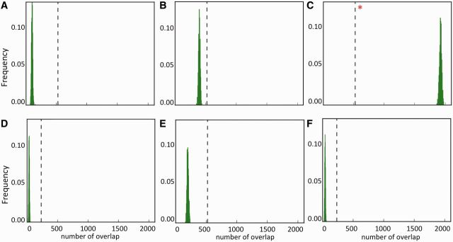
The expected null distributions can differ considerably under different permutation models. The pattern of co-occurrence of the binding sites of transcription factors STAT2 and CTCF in the human genome was analyzed. We shuffled the CTCF binding sites (A) unconstrained throughout the genome, (B) within certain distance (e.g. 1 kb) of their original locations to preserve domain level structures, (C) with other transcription factor binding sites present in the data set, as proposed by Haiminen et al., (D) only within gene promoters (5 kb upstream to 500 bp downstream of predicted transcription start sites of RefSeq genes), (E) after masking repressed domains as defined in the ENCODE project, (F) after masking repressed domains and shuffling only within the remaining gene promoters. The expected null distributions were generated by 1000 iterations under each model, and the observed overlap is shown as the vertical bar. In D–F, the extent of the observed overlap changed because of changes in the genomic regions analyzed. The observed overlap is significantly lower than that expected by chance under the null distributions A, B, D, E and F, but shows opposite trend under the null model C (shown with an asterisk).

CASE STUDY 2: PREVALENCE OF A G-QUADRUPLEX MOTIF FAMILY IN MOST CONSERVED ELEMENTS

Next, we investigated whether a family of G-quadruplex motifs, which play important roles in different biological processes such as transcription and replication and also in genomic instability [22], is significantly conserved during evolution. We obtained the set of G-quadruplex motifs, which were <20 bp in length [42], along with the most conserved regions with size <60 bp and conservation score >420 based on the alignment of 28 mammalian species from the UCSC genome browser [43]. We calculated the observed overlap of these sets of elements in the human genome. There were 35 014 G-quadruplex motifs and 28 800 most conserved elements in our data set. We then generated the expected null distributions by shuffling the G-quadruplex motifs (i) unconstrained across the genome, (ii) within 1 kb of their original locations to preserve the higher order domain-level organization (we obtained comparable results by shuffling within 5 kb and 10 kb of their original locations), (iii) only within respective chromosomes and after excluding centromere regions that are difficult to sequence and align and (vi) shuffling both the G-quadruplex motifs and also the most conserved elements, and thus ignoring the domain-level organization of these features. As shown in Figure 3, these permutation strategies produce slightly different null distributions, which affect the estimated enrichment and P-value of the observed overlap between G-quadruplex motifs and most conserved elements. We observed a moderately significant (P = 0.032) depletion of these motifs in most conserved elements under the null model C (Figure 3C), but it was not significant (P > 0.05) under other null models (including model B in Figure 3B, where we preserved the domain-level organization of G-quadruplexes during shuffling). In this particular case, we prefer the null model B over C, and accordingly report that the family of G-quadruplex motifs is not significantly depleted in the most conserved elements compared with that expected by chance (permutation P < 0.05) when the G-quadruplex motifs are shuffled within the chromosomes preserving the higher order domain-level organization. Once again, we underscore that the choice of the null model is nontrivial and can be debated; in any case, we advocate presenting the conclusions and the postulations of the null model clearly to avoid misinterpretation of the results.

Figure 3:

The statistical significance of overlap between G-quadruplex motifs of size <20 bp and most conserved elements of size <60 bp and conservation score >420 was tested using different permutation strategies (A–D). The expected null distributions were generated by 1000 iterations under each model, and the observed overlap is shown as the vertical bar. There was a significant depletion in overlap between these two features compared with that expected by chance in the null distribution generated using permutation model C, but the trend was not significant in other permutation models.

In summary, these two case studies highlight the impact of different permutation assumptions, and the dilemma it can potentially pose while interpreting the results in certain instances.

OUTLOOK

The case studies discussed earlier in the text show that there are different randomization methods for estimating statistical significance of genome-wide enrichment. In some cases, the choice among these options would be straightforward. In other cases, it might be nontrivial to identify the validity of the underlying assumptions and implement the ideal randomization strategy. In these cases, it would be important to describe the assumptions made in the null model, biological relevance of these assumptions and the potential caveats. Many studies have circumvented the dilemma of choosing the ideal randomization strategy by applying multiple randomization approaches and reporting P-value for each of these scenarios or the weakest P-value across different scenarios. Accepting the weakest P-value across different scenarios blindly might be unnecessarily conservative without a biological basis, and the former strategy might be a more rational approach. In those cases, where biologically relevant constraints are unclear, it will be preferable to examine whether key conclusions are consistent irrespective of the choice of randomization strategy.

Key Points.

• Statistical significance of nonrandom distribution of genomic and epigenomic features relies on the expected null distribution—typically generated using a permutation model.

• Different permutation models can generate different null distributions, leading to different levels of statistical significance of the observed features.

• The choice of a permutation model has the potential to influence key conclusions.

• In these cases, where biological constraints are unclear, it would be important to describe the assumptions made in the null model, biological basis of these assumptions, and the potential caveats.

FUNDING

NCI Physical Sciences Oncology Center pilot grant (U54CA143798), American Cancer Society grant (ACS IRG 57–001-53) and University of Colorado School of Medicine startup grants (to S.D.).

Biographies

Subhajyoti De is an Assistant Professor at University of Colorado School of Medicine. His research interests include cancer genomics, heterogeneous biological data integration and computational method development.

Brent S. Pedersen is a Senior Research Associate at University of Colorado School of Medicine. His research interests include genome-wide analysis and bioinformatics software development.

Katerina Kechris is an Associate Professor at Colorado School of Public Health. Her research interests include development and application of statistical methods for analyzing molecular sequences and high-throughput genomic data.

References

- 1.Hawkins RD, Hon GC, Ren B. Next-generation genomics: an integrative approach. Nat Rev Genet. 2010;11:476–86. doi: 10.1038/nrg2795. [DOI] [PMC free article] [PubMed] [Google Scholar]
- 2.Encode Project Consortium. Dunham I, Kundaje A, et al. An integrated encyclopedia of DNA elements in the human genome. Nature. 2012;489:57–74. doi: 10.1038/nature11247. [DOI] [PMC free article] [PubMed] [Google Scholar]
- 3.Lander ES. Initial impact of the sequencing of the human genome. Nature. 2011;470:187–97. doi: 10.1038/nature09792. [DOI] [PubMed] [Google Scholar]
- 4.Guttman M, Amit I, Garber M, et al. Chromatin signature reveals over a thousand highly conserved large non-coding RNAs in mammals. Nature. 2009;458:223–7. doi: 10.1038/nature07672. [DOI] [PMC free article] [PubMed] [Google Scholar]
- 5.Ernst J, Kellis M. Interplay between chromatin state, regulator binding, and regulatory motifs in six human cell types. Genome Res. 2013;23:1142–54. doi: 10.1101/gr.144840.112. [DOI] [PMC free article] [PubMed] [Google Scholar]
- 6.Ha N, Polychronidou M, Lohmann I. COPS: detecting co-occurrence and spatial arrangement of transcription factor binding motifs in genome-wide datasets. PLoS One. 2012;7:e52055. doi: 10.1371/journal.pone.0052055. [DOI] [PMC free article] [PubMed] [Google Scholar]
- 7.Klein H, Vingron M. Using transcription factor binding site co-occurrence to predict regulatory regions. Genome Inform. 2007;18:109–18. [PubMed] [Google Scholar]
- 8.Yip KY, Cheng C, Bhardwaj N, et al. Classification of human genomic regions based on experimentally determined binding sites of more than 100 transcription-related factors. Genome Biol. 2012;13:R48. doi: 10.1186/gb-2012-13-9-r48. [DOI] [PMC free article] [PubMed] [Google Scholar]
- 9.Beroukhim R, Getz G, Nghiemphu L, et al. Assessing the significance of chromosomal aberrations in cancer: methodology and application to glioma. Proc Natl Acad Sci USA. 2007;104:20007–12. doi: 10.1073/pnas.0710052104. [DOI] [PMC free article] [PubMed] [Google Scholar]
- 10.De S, Michor F. DNA secondary structures and epigenetic determinants of cancer genome evolution. Nat Struct Mol Biol. 2011;18:950–5. doi: 10.1038/nsmb.2089. [DOI] [PMC free article] [PubMed] [Google Scholar]
- 11.De S, Michor F. DNA replication timing and long-range DNA interactions predict mutational landscapes of cancer genomes. Nat Biotechnol. 2011;29:1103–8. doi: 10.1038/nbt.2030. [DOI] [PMC free article] [PubMed] [Google Scholar]
- 12.Navin N, Kendall J, Troge J, et al. Tumour evolution inferred by single-cell sequencing. Nature. 2011;472:90–4. doi: 10.1038/nature09807. [DOI] [PMC free article] [PubMed] [Google Scholar]
- 13.Zong C, Lu S, Chapman AR, et al. Genome-wide detection of single-nucleotide and copy-number variations of a single human cell. Science. 2012;338:1622–6. doi: 10.1126/science.1229164. [DOI] [PMC free article] [PubMed] [Google Scholar]
- 14.Fu AQ, Adryan B. Scoring overlapping and adjacent signals from genome-wide ChIP and DamID assays. Mol Biosyst. 2009;5:1429–38. doi: 10.1039/B906880e. [DOI] [PMC free article] [PubMed] [Google Scholar]
- 15.Haiminen N, Mannila H, Terzi E. Determining significance of pairwise co-occurrences of events in bursty sequences. BMC Bioinformatics. 2008;9:336. doi: 10.1186/1471-2105-9-336. [DOI] [PMC free article] [PubMed] [Google Scholar]
- 16.Mannila H, Toivonen H, Verkamo AI. Discovery of frequent episodes in event sequences. Data Min Knowl Discov. 1997;1:259–89. [Google Scholar]
- 17.Beroukhim R, Mermel CH, Porter D, et al. The landscape of somatic copy-number alteration across human cancers. Nature. 2010;463:899–905. doi: 10.1038/nature08822. [DOI] [PMC free article] [PubMed] [Google Scholar]
- 18.Quinlan AR, Hall IM. BEDTools: a flexible suite of utilities for comparing genomic features. Bioinformatics. 2010;26:841–2. doi: 10.1093/bioinformatics/btq033. [DOI] [PMC free article] [PubMed] [Google Scholar]
- 19.Dale RK, Pedersen BS, Quinlan AR. Pybedtools: a flexible Python library for manipulating genomic datasets and annotations. Bioinformatics. 2011;27:3423–4. doi: 10.1093/bioinformatics/btr539. [DOI] [PMC free article] [PubMed] [Google Scholar]
- 20.Sandve GK, Gundersen S, Rydbeck H, et al. The Genomic HyperBrowser: inferential genomics at the sequence level. Genome Biol. 2010;11:R121. doi: 10.1186/gb-2010-11-12-r121. [DOI] [PMC free article] [PubMed] [Google Scholar]
- 21.Treangen TJ, Salzberg SL. Repetitive DNA and next-generation sequencing: computational challenges and solutions. Nat Rev Genet. 2012;13:36–46. doi: 10.1038/nrg3117. [DOI] [PMC free article] [PubMed] [Google Scholar]
- 22.Huppert JL. Structure, location and interactions of G-quadruplexes. FEBS J. 2010;277:3452–8. doi: 10.1111/j.1742-4658.2010.07758.x. [DOI] [PubMed] [Google Scholar]
- 23.Layer RM, Skadron K, Robins G, et al. Binary Interval Search: a scalable algorithm for counting interval intersections. Bioinformatics. 2013;29:1–7. doi: 10.1093/bioinformatics/bts652. [DOI] [PMC free article] [PubMed] [Google Scholar]
- 24.Hannenhalli S, Levy S. Predicting transcription factor synergism. Nucleic Acids Res. 2002;30:4278–84. doi: 10.1093/nar/gkf535. [DOI] [PMC free article] [PubMed] [Google Scholar]
- 25.Bickel PJ, Boley N, Brown JB, et al. Subsampling methods for genomic inference. Ann Appl Stat. 2010;4:1660–97. [Google Scholar]
- 26.Haiminen N, Mannila H, Terzi E. Comparing segmentations by applying randomization techniques. BMC Bioinformatics. 2007;8:171. doi: 10.1186/1471-2105-8-171. [DOI] [PMC free article] [PubMed] [Google Scholar]
- 27.Braun JV, Muller HG. Statistical methods for DNA sequence segmentation. Stat Sci. 1998;13:142–62. [Google Scholar]
- 28.Dore LC, Chlon TM, Brown CD, et al. Chromatin occupancy analysis reveals genome-wide GATA factor switching during hematopoiesis. Blood. 2012;119:3724–33. doi: 10.1182/blood-2011-09-380634. [DOI] [PMC free article] [PubMed] [Google Scholar]
- 29.Euskirchen GM, Auerbach RK, Davidov E, et al. Diverse roles and interactions of the SWI/SNF chromatin remodeling complex revealed using global approaches. PLoS Genet. 2011;7:e1002008. doi: 10.1371/journal.pgen.1002008. [DOI] [PMC free article] [PubMed] [Google Scholar]
- 30.Giannopoulou EG, Elemento O. An integrated ChIP-seq analysis platform with customizable workflows. BMC Bioinformatics. 2011;12:277. doi: 10.1186/1471-2105-12-277. [DOI] [PMC free article] [PubMed] [Google Scholar]
- 31.Hoffman MM, Buske OJ, Wang J, et al. Unsupervised pattern discovery in human chromatin structure through genomic segmentation. Nat Methods. 2012;9:473–6. doi: 10.1038/nmeth.1937. [DOI] [PMC free article] [PubMed] [Google Scholar]
- 32.Margulies EH, Cooper GM, Asimenos G, et al. Analyses of deep mammalian sequence alignments and constraint predictions for 1% of the human genome. Genome Res. 2007;17:760–74. doi: 10.1101/gr.6034307. [DOI] [PMC free article] [PubMed] [Google Scholar]
- 33.Ross-Innes CS, Brown GD, Carroll JS. A co-ordinated interaction between CTCF and ER in breast cancer cells. BMC Genomics. 2011;12:593. doi: 10.1186/1471-2164-12-593. [DOI] [PMC free article] [PubMed] [Google Scholar]
- 34.Shibata Y, Sheffield NC, Fedrigo O, et al. Extensive evolutionary changes in regulatory element activity during human origins are associated with altered gene expression and positive selection. PLoS Genet. 2012;8:e1002789. doi: 10.1371/journal.pgen.1002789. [DOI] [PMC free article] [PubMed] [Google Scholar]
- 35.Chikina MD, Troyanskaya OG. An effective statistical evaluation of ChIPseq dataset similarity. Bioinformatics. 2012;28:607–13. doi: 10.1093/bioinformatics/bts009. [DOI] [PMC free article] [PubMed] [Google Scholar]
- 36.Huen DS, Russell S. On the use of resampling tests for evaluating statistical significance of binding-site co-occurrence. BMC Bioinformatics. 2010;11:359. doi: 10.1186/1471-2105-11-359. [DOI] [PMC free article] [PubMed] [Google Scholar]
- 37.Favorov A, Mularoni L, Cope LM, et al. Exploring massive, genome scale datasets with the GenometriCorr package. PLoS Comput Biol. 2012;8:e1002529. doi: 10.1371/journal.pcbi.1002529. [DOI] [PMC free article] [PubMed] [Google Scholar]
- 38.Purcell S, Neale B, Todd-Brown K, et al. PLINK: a tool set for whole-genome association and population-based linkage analyses. Am J Hum Genet. 2007;81:559–75. doi: 10.1086/519795. [DOI] [PMC free article] [PubMed] [Google Scholar]
- 39.Han B, Eskin E. Random-effects model aimed at discovering associations in meta-analysis of genome-wide association studies. Am J Hum Genet. 2011;88:586–98. doi: 10.1016/j.ajhg.2011.04.014. [DOI] [PMC free article] [PubMed] [Google Scholar]
- 40.Lau JF, Nusinzon I, Burakov D, et al. Role of metazoan mediator proteins in interferon-responsive transcription. Mol Cell Biol. 2003;23:620–8. doi: 10.1128/MCB.23.2.620-628.2003. [DOI] [PMC free article] [PubMed] [Google Scholar]
- 41.Phillips JE, Corces VG. CTCF: master weaver of the genome. Cell. 2009;137:1194–211. doi: 10.1016/j.cell.2009.06.001. [DOI] [PMC free article] [PubMed] [Google Scholar]
- 42.Huppert JL, Balasubramanian S. Prevalence of quadruplexes in the human genome. Nucleic Acids Res. 2005;33:2908–16. doi: 10.1093/nar/gki609. [DOI] [PMC free article] [PubMed] [Google Scholar]
- 43.Meyer LR, Zweig AS, Hinrichs AS, et al. The UCSC Genome Browser database: extensions and updates 2013. Nucleic Acids Res. 2013;41:D64–9. doi: 10.1093/nar/gks1048. [DOI] [PMC free article] [PubMed] [Google Scholar]