Choice certainty is informed by both evidence and decision time

Abstract

“Degree of certainty” refers to the subjective belief, prior to feedback, that a decision is correct. A reliable estimate of certainty is essential for prediction, learning from mistakes, and planning subsequent actions when outcomes are not immediate. It is generally thought that certainty is informed by a neural representation of evidence at the time of a decision. Here we show that certainty is also informed by the time taken to form the decision. Human subjects reported simultaneously their choice and confidence about the direction of a noisy display of moving dots. Certainty was inversely correlated with reaction times and directly correlated with motion strength. Moreover, these correlations were preserved even for error responses, a finding that contradicts existing explanations of certainty based on signal detection theory. We also contrived a stimulus manipulation that led to longer decision times without affecting choice accuracy, thus demonstrating that deliberation time itself informs the estimate of certainty. We suggest that elapsed decision time informs certainty because it serves as a proxy for task difficulty.

Introduction

Decisions are usually accompanied by a degree of certainty or confidence, which reflects a graded belief about the likelihood of different outcomes. Choice certainty plays at least two important roles. It facilitates adaptive regulation of behavior by furnishing a basis for learning from outcome (Dayan and Daw, 2008; Vickers, 1979), and it supports decision-making in complex environments where subsequent decisions depend on the predicted outcome of recent decisions before the actual consequences are known. For example, we tend to learn more from an erroneous decision about which we were more confident, and we tend to make conservative decisions if they depend on recent decisions whose outcomes are less certain (Kiani and Shadlen, 2009; Middlebrooks and Sommer, 2012).

How does a decision maker establish a degree of certainty? There are two potential sources of information. The first is rooted in the evidence; the second is associated with decision time. Because the state of the evidence contributes to choice accuracy, it seems likely that it might also bear on choice certainty. According to signal-detection theory (SDT) a choice is determined via comparison of a decision variable (DV) —a function of the evidence—to a criterion. It follows that the distance between the DV and criterion might underlie a judgment of certainty (Balakrishnan and Ratcliff, 1996; Ferrell, 1995; Kepecs et al., 2008; Treisman and Faulkner, 1984; Wallsten and Gonzalez-Vallejo, 1994). When the evidence strongly supports a choice, this distance is larger and the certainty is greater. Indeed, under a natural set of transformations, this distance is proportional to the log of a probability or likelihood ratio (Gold and Shadlen, 2001). Thus SDT and more sophisticated Bayesian classification schemes (Deneve et al., 2001; Jazayeri and Movshon, 2006; Ma et al., 2006; Zemel et al., 1998) provide a natural connection between choice and certainty since both depend on the probability that a decision is the correct one, based on the evidence.

However, SDT is inherently incapable of explaining systematic variations in the decision time (Baranski and Petrusic, 1994, 1998; Link, 1992; Ratcliff and Starns, 2009; Vickers and Smith, 1985). On the other hand, a variety of mechanisms resembling bounded evidence accumulation—diffusion, random walk, race and attractor models—produce highly successful accounts of both choice and reaction time (RT) for a multitude of perceptual and cognitive decisions (Beck et al., 2008; Churchland et al., 2008; Cisek, 2006; Donkin et al., 2011; Link and Heath, 1975; Purcell et al., 2010; Ratcliff and Starns, 2013; Reddi et al., 2003; Smith, 1988; Usher and McClelland, 2001; Vickers, 1979). This framework explains the relationship between speed and accuracy and is supported by neural recordings in the monkey (Bollimunta and Ditterich, 2012; Cook and Maunsell, 2002; Gold and Shadlen, 2007; Purcell et al., 2010; Ratcliff et al., 2007). The coupling between decision accuracy and decision time suggests that the latter might inform a judgment of certainty. Longer decision times are often associated with weaker sensory evidence and higher error rates. Thus, the brain may learn, by association, to use decision time or some function of it as a proxy for stimulus strength and certainty judgment.

The majority of theoretical accounts of choice certainty have ignored the temporal dynamics of the decision-making process. Like SDT, most bounded accumulation models attribute certainty to the state of the evidence at the time of decision (Beck et al., 2008; Petrusic and Cloutier, 1992; Van Zandt and Maldonado-Molina, 2004; Vickers, 1979; cf. Audley, 1960; Juslin and Olsson, 1997). To account for confidence, evidence must be accumulated by at least two competing mechanisms, because a scalar DV that terminates the decision at a criterion level cannot provide a graded representation of the evidence. Thus, choice certainty is thought to be based on the magnitude of evidence accumulated by the competing accumulators that do not reach the threshold and represent the losing alternatives (e.g., Beck et al., 2008; Pleskac and Busemeyer, 2010; Van Zandt and Maldonado-Molina, 2004; Vickers, 1979). These models predict a spurious correlation between certainty and RT, which is merely a reflection of an underlying correlation between stimulus difficulty (or accuracy) and RT. Accordingly, deliberation time itself is generally believed not to play a role in the computation of certainty.

For a large class of bounded accumulation models the relationship between the DV and accuracy is time dependent. That is, the same amount of accumulated evidence for a particular choice, but at different times, would be associated with different likelihoods that the choice is correct (Kiani and Shadlen, 2009). Therefore, a calculation of certainty based solely on the magnitude of a DV is suboptimal and can be adjusted by taking the passage of time into account. We hypothesized that both decision time and the state of the evidence leading to a choice affect subjective certainty, or confidence. Testing this hypothesis is not straightforward because decision time is usually affected by the evidence supporting a choice. Here, we disentangle the DV from decision time and show that certainty can be influenced by changes of decision time in the absence of a change in the DV and accuracy.

Results

Participants were asked to decide the direction of motion (up or down) in a dynamic, random-dot motion display. The strength of the motion varied randomly from trial to trial, and viewing duration was controlled by the subject. Whenever ready, the subject made a single saccadic eye movement to indicate both the direction choice and the degree of confidence that the choice was correct (Fig. 1B). The two choice-targets, corresponding to up and down, were shaped as rectangles, allowing subjects to indicate their certainty on a scale of uncertain to certain (left to right). Since saccadic eye movements are ballistic, the method ensures simultaneous reports of direction choice and its certainty.

Figure 1. Choice-reaction time task with simultaneous report of choice and certainty.

A. Stimulus display. Observers reported the direction of dynamic random dot motion (up or down) and choice certainty by making a single saccadic eye movement to one of the two bar-shaped targets. The landing point of the saccade along the target indicated the degree of certainty, which ranged from guessing (red) to full confidence (green). B. Task sequence. After acquiring a fixation point the two targets appeared on the screen, followed by the motion stimulus. The subject made a saccadic eye movement when ready. The motion stimulus was extinguished when the observer initiated an eye movement. C. Probability correct and reaction time conformed to expectations of a bounded accumulation mechanism (see Methods). Each column shows data from one subject (S1–S6). The model was fit to the overall distribution of RTs. Then the parameters were used to predict the subject’s accuracy (gray curves, upper panel) and the correct RTs (solid black curves, lower panel). Error bars are s.e.m.

In the direction discrimination task, stronger motion led to improved accuracy and faster RTs (Fig. 1C), as previously shown (Churchland et al., 2008; Ditterich et al., 2003; Huk and Shadlen, 2005; Palmer et al., 2005; Roitman and Shadlen, 2002). The relationship between choice and RT is explained by a bounded accumulation model (see Methods). The curves in Fig. 1C are predictions of a model that was fit using only the observed distribution of RTs, irrespective of choice (Fig. S1). The predictive power of this model is remarkable, but the important point for our purpose is that the relationship between RT and probability correct is so strong that the expected accuracy can be predicted based only on RTs. We hypothesized that the brain might therefore exploit this relationship for certainty judgments.

The measure of certainty was the horizontal end point of the subject’s saccade. Of course we cannot know how a subject maps an estimate of the probability she will be correct into a horizontal position along the target. We assume only that the expectations of these horizontal positions are monotonically related to confidence. Indeed Figure 2A is consistent with this assumption. For correct responses, saccadic endpoints along the horizontal dimension were monotonically related to motion strength (p<10⁻⁸ for all subjects) (Balakrishnan and Ratcliff, 1996; Green and Swets, 1966; Vickers, 1979). The more important observation is the inverse relationship with RT. This is evident by the downward trend of the traces in Figure 2A (Eq. 4, p<10⁻⁸ for all subjects). The effects of both coherence and RT were seen in all six observers, albeit to different degrees. The effect of motion strength is masked for subjects 1 and 4 because these subjects utilized a limited range of saccade end points. However, zooming in clarifies both effects (Fig. S2). Overall, neither the effect of RTs nor the effects of motion strength could be described by the other one. That is, for a fixed RT, trials with lower stimulus strength had lower choice certainty, and for a fixed stimulus strength, trials with longer RTs had lower choice certainty.

Figure 2. Certainty varies as a function of both RT and motion strength. Each column shows data from one subject (S1–S6).

A. Certainty on correct choices. The horizontal position of the saccade end points are grouped by motion strength and RT. Positive endpoints connote greater certainty. For 0% coherence all trials are included. RTs are grouped in quintiles for each motion strength. B. Certainty on errors. Error bars are s.e.m.

Due to the stochastic nature of the random dot stimulus, the experienced strength of motion fluctuates from trial to trial even for the same motion coherence. We performed two control analyses to test whether random variations of the stimulus strength could explain away the relationship of RT with certainty. First, on a subset of trials we showed an identical sequence of random dot motion to the subjects. These trials replicated the independent effects of reaction time and motion strength on certainty (p<10⁻⁸ for RT and p<10⁻⁵ for motion coherence; see Methods and Fig. S3). Secondly, we quantified trial-to-trial fluctuations of stimulus strength by calculating motion energy for trials in which the motion sequence was not fixed (see Methods). Subjects’ certainty increased with the average motion energy (Fig. 3; Eq. 9, p<10⁻⁴ for all subjects) or the integral of motion energy (Fig. S4; Eq. 9, p<10⁻⁸ for all subjects) on each trial. However, for each motion energy, certainty remained inversely correlated with RT (Eq. 9, p<10⁻⁸ for all subjects, both for the average and the integral of motion energy), suggesting that the relationship between certainty and RT was not due solely to random variations of motion strength for each coherence.

Figure 3. The inverse relationship between RT and certainty is not explained by trial-to-trial fluctuations of the random dot stimulus. Each column represents data from one subject (S1–S6).

For each subject and response condition (correct or error), trials are grouped into quintiles based on RTs (indicated by color). Each RT group is further divided into quintiles based on average motion energy (filled circles). A. Correct trials. Certainty grows with average motion energy but for each average motion energy longer RTs are associated with lower certainty. B. Error trials. For each level of motion energy, certainty is inversely related to RT. Error bars are s.e.m.

The inverse relationship between choice certainty and RT was also evident when subjects made errors (Fig. 2B). Compared to correct responses, RTs were longer for error responses (t-test, p<10⁻⁶, 13%–65% increase across subjects), and the error certainties were smaller accordingly (p<0.002)(Petrusic and Cloutier, 1992; Pierrel and Murray, 1963; Vickers and Smith, 1985). Importantly, among the error responses themselves, subjects were more confident about faster errors (Eq. 4, p<10⁻⁴). Indeed, for five of six subjects, the regression slopes of saccadic endpoint versus RT were statistically indistinguishable from the regression slopes for correct responses (Eq. 5, p>0.3 for five subjects, for subject 2, p=0.001). Finally, the certainty associated with errors was greater when subjects viewed stronger motion (Fig. 4; Eq. 6, p<0.05 for five subjects, p=0.002 for pooled data). This last observation is critical for establishing a close link between RT and certainty beyond that implied by stimulus difficulty and accuracy, because it contradicts predictions from SDT and many explanations of confidence ratings based solely on the state of the DV that underlies the choice, as we elaborate in Discussion.

Figure 4. Certainty grows with stimulus strength for both correct and error responses.

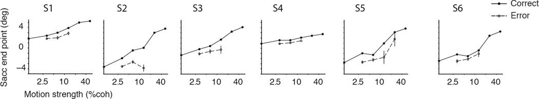
A. The horizontal position of the saccade end points are averaged across all RTs for the correct (solid) and error (dashed) responses for each motion strength. Overall, subjects were less certain when they made errors, but five of the six subjects were more certain when those errors were made in response to stronger motion. Each panel shows the data from one subject (S1–S6). Error bars are s.e.m.

The same bounded accumulation model that predicted subjects’ accuracy based on their RT distributions also predicted the increase of certainty with motion strength for both the correct and error trials. The key insight is that both the DV and time convey information about certainty in the model. The model consists of two competing accumulators, which integrate noisy momentary evidence (Fig. 5A). The noisy inputs of the two accumulators may not be perfectly correlated, thereby giving rise to a pair of DVs that are not completely redundant (Fig. 5B). The accumulator that reaches its upper bound faster dictates the choice and the decision time. Note that the winning accumulator is not informative for the computation of certainty because it is always at a bound at the time of the decision. However, the losing accumulator can contribute to the certainty computation (Vickers and Packer, 1982). The losing accumulator confers greater confidence the farther it is from the upper bound. However, the mapping between the DV of the losing accumulator and the probability that the response will be correct varies with elapsed decision time (Fig. 5C–D). For example, an intermediate or low DV in the losing accumulator for an early decision forecasts a higher likelihood of success than later on.

Figure 5. A simple bounded accumulation model predicts choice, RT, and certainty.

A. The model. Two accumulators compete by integrating noisy momentary evidence in favor of the two choices. Momentary evidence (e₁, e₂) is drawn from a bivariate normal distribution. The accumulator that first reaches the absorbing bound dictates the choice and decision time. B. The choices and decision times of the model across trials can be formalized by propagation of a probability distribution over time in the space confined by the bounds of the two accumulators. The figure shows the joint distribution of decision variable at 1 s for upward 12.8% coherence. The correlation between e₁ and e₂ is −0.79. C. At the time of the decision, the DV of the winning accumulator (v_j) is at the upper bound, but the DV of the losing accumulator (v_i) can span a range of values. Panels depict DV distributions associated with correct and incorrect choices for the same motion strength as in B. Note that the distribution depends on decision time. D. The probability of a correct response depends on both the decision variable and decision time. Colors correspond to the log odds of a correct response across all motion strengths (Eq. 3). The inverted wedge at the left side of the figure corresponds to combinations of the DV and decision time that have extremely low probabilities. Termination of the decision-making process in that region is due to noise and unlikely to lead to better-than-chance accuracy. Combinations of the DV and decision time to the right of the wedge are much more likely and show the dependence of expected accuracy on the DV and time. E. Model predictions for the subject’s certainty. The model parameters were estimated by fitting the overall distribution of RTs, irrespective of choice and certainty (same parameters as those used in Fig. 1C). These parameters were then used to predict the model certainty for correct and error choices as a function of motion strength. The exact mapping between certainty and saccade landing positions varies from subject-to-subject, as expected from idiosyncratic interpretation of task instructions. However, the model correctly predicts the form of the certainty functions for each of the six subjects (Fig. 4). F. Fit of the model’s predicted certainty to confidence ratings. For each subject, we assume a monotonically increasing relationship between saccade end point and certainty.

We hypothesize that the brain can learn these associations and use them for efficient computation of certainty. The smoothness of changes of the log odds of success with time and DV (Fig. 5D) supports the plausibility of this hypothesis. In particular, the associations have a low dimensional parameterization, suggesting they can be learned from limited samples (i.e., experience). The model prediction for the subject’s expected certainty for each motion strength can be formalized as the subject’s expected probability to respond correctly based on (i) the learned association of accuracy with the DV and decision time, (ii) the predicted distribution of reaction times, and (iii) the predicted distribution of the DV of the losing accumulator. The expected certainty for each motion strength on correct and incorrect trials is given by:

$$\mathrm{p̂}(\mathit{\text{cor}}|C,R)=\underset{t}{\int }p(t|C,R)(\underset{v}{\int }\mathrm{p̂}(\mathit{\text{cor}}|\mathrm{v⃗},t)p(\mathrm{v⃗}|t,C,R)dv)dt$$

where C is the motion strength, t is the decision time, and R is the observed response from the experimenter’s perspective (correct or error). p̂ (cor | v⃗, t) represents the learned association between the experienced correct feedback and the decision time and DV. Note that all components of the equation above can be readily calculated with the model parameters obtained from the RT distributions (Fig. 1C). Figure 5E shows these predictions. A comparison with Fig. 4 reveals the model’s success in predicting the certainty. In fact, by assuming a monotonic relationship between the model’s predicted certainty and the landing points of subjects’ saccades we can provide a good fit to the observed responses (Fig. 5F).

A causal test of the effect of elapsed time on the computation of certainty

Our results suggest that certainty does not derive merely from the state of the DV guiding the choice, but from some other cue about difficulty. Based on the link between RT and certainty, the additional source of information could be decision time or a monotonic function thereof (e.g., rate of evidence accumulation). However, decision time is closely linked to accuracy (Fig. S5; Eq. 7, p<0.0005). In principle, any factor that affects probability correct could affect certainty and thereby induce a spurious relationship between certainty and RT. To establish that certainty judgments are directly influenced by decision time, we need to isolate changes of RT from probability correct and demonstrate that even when probability correct remains the same, subjects are less confident about late responses.

To achieve this, we developed a stimulus manipulation using the following strategy. If a decision is based on accumulation of evidence over time it ought to be possible to prolong the decision process by providing evidence that cancels previous evidence (Fig. 6). The random dot motion stimulus is ideal for this purpose. The stimulus is inherently stochastic: even for a fixed coherence level, the actual motion energy fluctuates over time during a trial. This feature permits a stealthy modification of the stimulus by introduction of specific sequences of motion, tailored to cancel the evidence provided by an earlier portion of motion stimulus. On half of the trials with 0% or 3.2% coherence, we introduced a 160 ms long cancellation pulse by playing in reverse order the motion frames immediately preceding the pulse (Fig. 6A)(see Methods). We limited the reverse pulses to the weakest stimuli to keep subjects’ experiences as close to normal as possible and thus prevent deliberate changes of decision strategy. None of the subjects reported unexpected changes of the stimulus in the debriefing after the experiment. That is, stimulus fluctuations caused by the reverse pulse were within the range of experienced fluctuations in other trials. Through introduction of reverse pulse we tried to return the accumulated evidence to its value at a previous point in time, thereby allowing the decision process to continue as if the previous 360 ms achieved no net change in evidence favoring either direction. The manipulation only approximates this goal, but under reasonable assumptions, it ought to lead to no net change in the probability correct.

Figure 6. Decoupling RT and accuracy via insertion of a “reverse pulse”.

On half of the trials for the two lowest motion strength (0% and 3.2% coherence) a 160 ms pulse of reverse motion was presented to cancel the evidence from the preceding stimulus. A. The reverse pulse causes approximate cancellation of the immediately preceding motion sequence. Traces show average motion energy profiles for 3.2% coherence trials for 360 ms of normal stimulus (blue) or a 160 ms reverse pulse following 200 ms of normal stimulus (red). Positive values correspond to the correct direction, which is opposite to the reverse pulse. Shaded area represents s.e.m. In a bounded accumulation model, the reverse pulse is expected to increase RT without changing the proportion of correct choices. B. Probability correct and reaction times in the presence (gray) and absence (white) of reverse pulse. Each column displays data from one subject. Error bars show s.e.m.

Five subjects were tested in this experiment. As expected, the reverse pulse led to increased RT (Fig. 6B). The RT changes varied across subjects, owing presumably to different tendencies to censor long RTs (Churchland et al., 2008; Drugowitsch et al., 2012), but the size of the change was considerable (222.6±68.6 ms, mean±s.e.m. across subjects; ANOVA p<0.005 for all subjects except S2; p<10⁻⁸ for pooled data from all subjects). Despite these longer RTs, the probability correct for 3.2% coherence did not show an appreciable change (Z-test for proportions, p>0.2 for each subject). It seems unlikely that this is explained by lack of power because (i) the change was also undetectable in pooled data from all subjects (p=0.48; 1395 trials, a change of accuracy as small as 0.045 would yield p≤0.05) and (ii) the probability correct for the 3.2% coherence (74%–81%) is close to the mid-point of the psychometric function, where it is steepest, permitting easy detection of a stimulus-induced change. In other words, we optimized the experiment as well as possible to detect small changes of accuracy.

Although the reverse pulse failed to affect accuracy, it reduced the subject’s confidence (Fig 7A; ANOVA, p<0.05 for each subject except S4; p=10⁻⁷ for pooled data). The reduction of certainty was most pronounced for 3.2% coherence trials. On 0% coherence trials the reported certainty in the absence of reverse pulse was already near the minimum of the range utilized by each subject. Nonetheless, the effect was evident even for the 0% coherence strength when the data were pooled across subjects (p=0.006, Wilcoxon rank sum test). The reduction in certainty is remarkable in light of the subtlety of the stimulus manipulation—brief pulses applied only to the weakest stimuli. Indeed, the manipulation resembled the stochastic variations already present in the stimulus, which explains why they were not apparent to subjects.

Figure 7. The reverse pulse reduced choice certainty. Each column represents one subject.

A. Certainty judgments with and without a reverse pulse. Bar graphs show the average horizontal position of saccadic end points in the presence (gray) and absence (white) of the reverse pulse. Error bars represent s.e.m. All 0% coherence trials and correct 3.2% coherence trials are shown. B. Change of saccade end points as a function of reaction time and motion strength in the presence (solid symbols) and absence (hollow symbols and dashed line) of reverse pulse. Conventions are similar to Fig. 2A.

Although the changes in accuracy did not reach significance, we worried that Fig. 6 suggests a trend towards reduced accuracy. To explore whether this trend can account for the significantly reduced confidence we estimated the expected change in saccadic landing position based on the monotonic relationship between accuracy and certainty. In four of the five subjects the reverse pulse affected confidence to a greater degree than one would anticipate from the empirical relationship between accuracy and confidence (p<0.05 for all subjects but S4; p<10⁻⁴ for pooled data). Moreover, the reduction in certainty was compatible with the increased RTs (Fig. 7B). The slope of the regression for certainty vs. RT was unchanged (Eq. 8, p>0.3 for each subject; p=0.25 for the pooled data). In other words, the reverse pulse reduced choice certainty by the amount expected for the change of RT.

From this experiment we conclude that a variation of decision time that is not associated with a change in accuracy is itself sufficient to induce changes in confidence. On the other hand, the first experiment indicates that decision time alone is insufficient for explaining confidence. Together, these experiments show that both elapsed decision time and the state of accumulated evidence shape the sense of certainty. The bounded accumulation model successfully formalizes this relationship.

Discussion

Traditionally, quantitative studies of perception were based on three behavioral measurements: accuracy, RT and confidence ratings. A longstanding goal seeks to relate these measures to the underlying decision process. All three measures are affected by stimulus strength or difficulty. Although accounting for the exact quantitative relationships is nontrivial, it seems natural that a low quality of evidence, defined by low signal-to-noise ratio (SNR), would be associated with worse accuracy, slower response times and lower confidence ratings. Indeed, if certainty is at all meaningful, it ought to reflect accuracy, on average, even if imperfectly (Drugowitsch et al., 2014). This trend, which is apparent in our experiment, reassures us that our subjects’ reports of certainty were sensible.

The main finding from our study is a critical role of elapsed time on judgments of certainty. Psychologists have long known that longer RT may be associated with lower confidence ratings (Audley, 1960; Baranski and Petrusic, 1998; Henmon, 1911; Johnson, 1939; Volkmann, 1934), but it is often assumed this association merely reflects task difficulty and accuracy. Since decision time is naturally correlated with both of these variables, there has been little interest in the idea that time itself might affect the sense of certainty. However, recent experiments using post-decision wagering in nonhuman primates suggest that both accumulated evidence and elapsed decision time are combined to inform a sense of certainty in a decision (Fetsch et al., 2014; Kiani and Shadlen, 2009). Post-decision wagering is an indirect proxy for certainty, which cannot be ascertained directly in animals. The present study solicits a more direct “rating scale” measure of certainty from humans, and it exploits two task manipulations, which allowed us to deduce decision times on single trials and to dissociate decision time from accuracy. These manipulations are the simultaneous report of direction and confidence and a stimulus modification that effectively adds time but no information to the evidence.

We used a choice-reaction time paradigm to study a perceptual decision that is known to rest on the accumulation of sequential samples of evidence in time. We confirmed that a mechanism like bounded evidence accumulation accounts for the speed and accuracy of subject’s decisions, consistent with previous experiments in human and nonhuman primates. The reaction times are short compared to cognitive decisions, but they are long compared to many perceptual categorizations, because they require integration of evidence over time to achieve an acceptable level of accuracy. The capacity to predict subjects’ accuracy from measurements of their RT (Fig. 1C gray curves) is testimonial to the explanatory power of this model framework. It indicates that we can deduce the decision time of our subjects from their measured RT.

One of the novel task innovations ensured that subjects used the same information to make their direction choice and confidence rating (Ratcliff and Starns, 2013). Although the stimulus motion is turned off at the moment the subject initiates their eye movement response, we have shown elsewhere that the brain does not utilize the final ~0.3 sec of stimulus information in this choice. Since, the additional information can be used to revise an initial choice (Resulaj et al., 2009), we wished to suppress the possibility that subjects would base a confidence rating on this additional information. We achieved this by using a single ballistic eye movement to indicate both choice and confidence. In supplementary information (Fig. S6), we show that a serial report of choice followed by confidence replicates our main findings. However, we suspect that this would not be the case if we had tested decisions that use shorter temporal integration periods, for which a few extra tenths of seconds of information might dissociate choice and confidence when they are reported serially. Further, we expect that a serial report of choice and confidence would significantly reduce the utility of error trials for inferring the mechanism of confidence (Fig. 4) simply because subjects could use the period between the choice and confidence report to recalibrate their confidence or even change their minds (Caspi et al., 2004; Kiani et al., 2014; Resulaj et al., 2009). For example, serial reporting of choice and certainty might weaken or even reverse the trend in Figure 4.

All six subjects support our conclusion that certainty is shaped by both decision time and the state of the evidence represented by the losing accumulator. While both factors were required to explain the data from each of the six subjects, some were more affected by decision time than motion strength (e.g., S1; Fig 2A), whereas others were more affected by motion strength (e.g., S2), hence the state of the losing accumulator. In our model, this is captured mainly by the level of correlated noise in the two DVs and also by the reflecting lower bounds (Fig 5A). We expect the sign of correlation to be negative because some of the noise derives from the random dot stimulus itself (Bollimunta and Ditterich, 2012). Were the two DVs exact inverse replicas (i.e., correlation = −1) there would be no information obtainable from the losing accumulator, leaving decision time as the sole determinant of certainty. This possibility is inconsistent with the data, although it is the usual depiction of bounded evidence accumulation on a single graph with symmetric choice bounds.

A single accumulator with two bounds (aka, diffusion model) has often been adopted for mathematical convenience, not for its biological plausibility. Indeed, electrophysiological experiments suggest an array of accumulators that compete with each other (Beck et al., 2008; Bogacz et al., 2007; Bollimunta and Ditterich, 2012; Churchland et al., 2008; Mazurek et al., 2003; Usher et al., 2013). For binary choices, if one assumes perfect anti-correlation between two accumulators, two competing accumulators may be depicted as a single accumulation toward or away from upper and lower bounds. Such bounded accumulation is sufficient to explain many aspects of choice and RT. However, it is insufficient to explain concurrent effects of accumulated evidence and decision time on confidence, because this simple model would imply incorrectly that the only information supporting confidence is the decision time. An additional, partially independent process is essential to explain the effect of accumulated evidence. We assume that this is the losing race (Vickers and Packer, 1982), but it could be any competing process. Thus our model is related to a variety of race models (e.g., Brown and Heathcote, 2008; Donkin et al., 2011). Importantly, taking elapsed time into account improves the computation of certainty in all such models.

In our second experiment, we attempted to achieve the dissociation of certainty and accuracy by reversing the accumulated evidence—returning it to its state 160 ms ago. The strategy contains an obvious flaw: the reverse pulse does not cancel the neural noise in the brain. Neural firing rates fluctuate randomly even for a fixed stimulus (Britten et al., 1993; Schiller et al., 1976; Shadlen and Newsome, 1998; Snowden et al., 1992; Tolhurst et al., 1983; Vogels et al., 1989), and these random fluctuations continue to accumulate during the reverse pulse, leading to a larger dispersion of accumulated evidence. Even stimulus noise is not perfectly canceled (e.g., adjacent frames are not reversed; see Methods). Our attempt, therefore, was only approximate. Nonetheless, the lack of change in probability correct achieves the important goal: a change in RT without a change in the probability correct. The latter is not explained by a lack of statistical power. The probability correct (74%–81%) coincides with the steepest part of the psychometric function (Figs. 1 & 6), where the likelihood of detection of a change in accuracy ought to be maximal. Moreover, the change in certainty cannot be explained by the small and insignificant variations of accuracy, whereas it is fully compatible with the increased RT (Fig. 7). Overall, the reverse pulse experiment suggests that manipulation of decision time itself is sufficient to affect confidence.

How is a degree of certainty assigned on a single decision? The probability of a correct decision is reflected in the proportion of correct choices, but any one decision is either correct or not. Standard decision theory furnishes an adequate account of how such proportions arise based on simple considerations of signal and noise (Britten et al., 1992; Green and Swets, 1966; Tolhurst et al., 1983), but most are found wanting when attempting to account for the graded degree of certainty on a single trial. For example signal detection theory posits that a decision is based on the comparison of a DV to a criterion, and the distance from the criterion underlies certainty (Balakrishnan and Ratcliff, 1996; Ferrell, 1995; Kepecs et al., 2008; Treisman and Faulkner, 1984; Wallsten and Gonzalez-Vallejo, 1994). As the stimulus strength increases, the DV distribution systematically shifts to one side of the criterion. As a result, the mean of the DVs on the “correct” side of the criterion increases, causing an increase of certainty for correct responses with stronger stimuli. However, the mean of the DVs on the wrong side of the criterion decreases, suggesting a reduction of error certainty with stimulus strength (Kepecs et al., 2008; Kim and Shadlen, 1999). Therefore the relationship between difficulty and certainty should reverse on errors. A similar prediction is made by the majority of accumulation models that attribute certainty to only the DV (Ratcliff and Starns, 2013; Rolls et al., 2010; Vickers, 1979; Zylberberg et al., 2012). This prediction is contradicted by our data (Fig. 4; but see the note above on the importance of simultaneous report of choice and certainty). We wish to emphasize that our model does not overturn SDT. We view sequential sampling as a natural extension of SDT to explain the time taken to reach a decision (e.g., speed vs. accuracy). In so doing, it provides a novel account of decision confidence.

Most extensions of SDT, which account for both RT and accuracy, attribute certainty judgment to the level of evidence supporting each choice (but see Audley, 1960). Accordingly, certainty must reflect the probability correct. For example, in Vickers’ balance-of-evidence model (Vickers, 1979; Vickers and Smith, 1985), confidence is a monotonic function of the difference of accumulated evidence for the chosen option and alternative option(s). Recent models based on a Bayesian theory of decision-making (e.g. Beck et al., 2008; Ma et al., 2006) extend this framework to approximate a posterior probability distribution from an assembly of accumulators. All such models suggest that the level of certainty is closely related to probability correct (but see Drugowitsch et al., 2014). Moreover, since probability correct is lower on more difficult trials, which are associated with longer RTs, these models also predict an empirical relationship between decision time and confidence, similar to those in Fig. 2A. The similarity is superficial, however, because it is explained by difficulty— motion coherence in our study. Our second experiment demonstrates that even in the absence of a change in probability correct, elongation of RT leads to lower confidence about motion direction. On the other hand, our first experiment shows that RT alone cannot explain variations in certainty. Confidence is therefore informed by both the DV that supports a choice—both the winning and losing accumulators—and the time taken to achieve that DV.

In hindsight, it seems obvious that the brain would exploit elapsed time as a source of information. Certainty (or confidence) is something a decision maker experiences on a single choice. In addition to deciding what is the correct choice, the decision-maker must ascertain whether the evidence derives from a reliable or unreliable source. This is not easily ascertained from the evidence alone. Within the framework of bounded accumulation, decision time confers an important clue to reliability for the simple reason that more reliable evidence leads to faster decisions. In these models, the mapping between the DV and accuracy is time dependent (Kiani and Shadlen, 2009). This time dependence can be learned and exploited by the brain to calibrate the sense of confidence. Currently, it is unclear whether this insight extends to more complex decisions that occur over longer time scales. However, for simple perceptual decisions that form in a fraction of a second to a few seconds, keeping track of the decision time and using it to calibrate the sense of certainty provides a computational shortcut.

It seems possible that neurons in the lateral intraparietal area (LIP) furnish a representation of the state of evidence (Churchland et al., 2008; Gold and Shadlen, 2007; Roitman and Shadlen, 2002). Indeed, the same LIP neurons have been shown to represent elapsed time when an animal must base a behavior on this quantity (Janssen and Shadlen, 2005; Leon and Shadlen, 2003). It remains to be seen how evidence and elapsed time are combined to support a level of confidence. Neurons in orbitofrontal (Kepecs et al., 2008; Padoa-Schioppa and Assad, 2006) and cingulate cortex (Hayden et al., 2008) have been suggested to represent the outcome of this computation and may be performing the computation. The idea that elapsed time affects certainty judgments leads us to suspect that the brain must represent probability, implicitly at least, in a dynamic sense. Elapsed time during a decision is impetus to discount the belief that a hypothesis is true, given the data (Hanks et al., 2011; Shadlen et al., 2006).

Methods

Observers

Six young adult human subjects (four males and two females) participated in the experiments. Five were naïve to the purpose of the experiment. Observers had normal or corrected-to-normal vision, and, except for one subject, had been extensively trained on the direction discrimination task prior to data collection. Informed written consent was obtained from the subjects. All experimental procedures were approved by the institutional review board at the University of Washington.

Eye monitoring

Eye movements were recorded noninvasively using a high-speed infrared eye-tracking device (Eyelink 1000, SR Research) controlled by a dedicated host PC. Subjects were seated in an adjustable chair in a semi-dark booth, with their chin and forehead resting on a tower-mount chinrest. Prior to data collection, the system was calibrated by showing 9 targets at center, edges and corners of the display monitor. During data collection, gaze position of the left eye was sampled at 500 Hz, saved on the host PC and passed to the experimental control computer via Ethernet link. The system operated in a pupil-corneal reflection mode, and had an average accuracy of 0.25°−0.5°. We monitored the eye position to ensure fixation during stimulus viewing (window 4×4 deg²) and to achieve precise measurements of choice-reaction times (see below).

Behavioral tasks

Each trial started when the subjects maintained fixation on a circular fixation point (FP, 0.3° diameter) at the center of the display monitor (17˝ flat-screen CRT; View Sonic PF790; refresh rate, 75 Hz; screen resolution 800×600; viewing distance, 57 cm). Immediately, two targets appeared 8° above and below the FP to indicate the two possible motion directions (upward or downward). Each target was a horizontal rectangle (0.5° by 9°) shaded from red on the left side to green on the right side (Fig. 1A). After a short delay (200–500 ms, truncated exponential distribution), dynamic random dot motion was displayed in a virtual aperture (5° diameter) centered at the FP. The dots were white squares (0.088° per side) on a black background. The dot density was 16.7 dots/deg²/s. The stimulus is described in detail elsewhere (Shadlen and Newsome, 2001). It consisted of three independent sets of dots shown on consecutive video frames. The strength of motion was controlled by adjusting the probability that a dot displayed in a video frame would be displaced by Δy in a video frame 40 ms later (i.e., 3 video frames). The intervening frames contained independent sets of dots. The displacement, Δy, was consistent with a speed of ±5 deg/s. Dots that were not displaced were replaced by a dot at a random location in the aperture. We refer to this displacement probability (times 100) as motion strength or coherence. Matlab code for generating the display is freely available as an add-on to the psychophysics toolbox (Brainard, 1997).

Motion direction and strength varied randomly from trial to trial. For half of the trials we removed trial-to-trial variability of motion stimulus by using a predetermined seed (one per coherence and direction) to initiate the random number generator. For the other half of trials the seed was chosen randomly. The subjects were asked to report motion direction when ready by making a saccadic eye movement to the corresponding target and maintaining stable fixation on the target for 500 ms. They were instructed to report choice certainty by directing the same saccade along the horizontal dimension of the target. The choice certainty scaled from most uncertain (guessing) on the left edge of target (red color) to most certain (100% confident) on the right edge (green color). Saccadic end point along the chosen target was defined as the average eye position in a 200 ms window toward the end of the fixation period. The random dot stimulus was extinguished when the gaze left the central fixation window. Auditory feedback was delivered for correct and error choices irrespective of the subject’s reported certainty. On trials with 0% coherence the subject randomly received the correct feedback on half of the trials. RT was calculated as the time from motion onset to saccade initiation, which was detected when the gaze first exited the fixation window. In the first experiment, we collected 7 to 15 blocks of data, each consisting of 200 trials, from each subject.

In the second experiment, on half of the trials with 0% or 3.2% motion coherence, a 160 ms long reverse pulse was presented at a random time starting 200 ms to 400 ms after the stimulus onset. The reverse pulse was a sequence of 12 frames of the immediately preceding stimulus played in reverse order. The reverse play was performed within each independent set of dots (see above). Let A_i, B_i and C_i represent a set of three temporally adjacent, independent frames, where the subscript defines the 40 ms epoch. A sequence of frames for the reverse pulse and the preceding stimulus is A₁ B₁ C₁ A₂ B₂ C₂ A₃ B₃ C₃ A₄ B₄ C₄ A₅ B₅ C₅ A₄ B₄ C₄ A₃ B₃ C₃ A₂ B₂ C₂ A₁ B₁ C₁, which spans 360 ms. Because the pulse was presented only on weak motion trials, it did not produce perceptible changes in the stimulus. None of the subjects reported any noticeable stimulus change compared to the first experiment in the briefing after the experiment. We collected 5 to 12 blocks of data, each consisting of 200 trials, from each subject.

Bounded accumulation model

The diffusion model used to fit the RT data in Fig. 1C assumes a race between two accumulators that represent the available choices. Each accumulator integrates momentary evidence toward a decision bound. The accumulator that reaches the bound first dictates the choice. The momentary evidence to the two accumulators is represented by a bivariate Normal distribution with mean μ⃗ = [kC, −kC] and covariance matrix $V=\left[\begin{array}{cc}\hfill 1\hfill & \hfill r\hfill \\ \hfill r\hfill & \hfill 1\hfill \end{array}\right]$, where k translates motion strength (C) to the mean of momentary evidence, and r defines the input correlation of the two accumulators. The duration of the accumulation process is termed decision time, and the accumulated evidence is termed the decision variable. The propagation of the probability density of the decision variable over time can be calculated using a simplified two-dimensional Fokker-Planck equation:

$$\frac{\partial p(\mathrm{v⃗},t)}{\partial t}=-\sum _{i=1}^2{\mu }_i\frac{\partial p(\mathrm{v⃗},t)}{\partial v_i}+\sum _{i=1}^2\sum _{j=1}^2{D}_{ij}\frac{{\partial }^{2}p(\mathrm{v⃗},t)}{\partial v_i\partial v_j}$$ (1)

where p(v⃗, t) is the probability of the decision variable vector v⃗ at time t, and $D_{ij}=0.5\sum _{m=1}^2{\sigma }_{im}{\sigma }_{jm}$. The boundary conditions of the Fokker-Planck equation are:

$$p(\mathrm{v⃗},t_0)=\delta (v_1)\delta (v_2)p(v_i(t)=B_u,t)=0$$ (2)

where δ (·) is the Kronecker delta function. The first condition constrains the initial value of the decision variable to zero for both accumulators. The second condition enforces that the accumulation terminates whenever an accumulator reaches its “absorbing” upper bound (B_u). Additionally, we assumed that each accumulator has a lower reflective bound (B_l) that prevents very low accumulated evidence; just as neural responses are bounded from below. In addition to its biological appeal, this lower reflective bound facilitates the numerical solution of the Fokker-Planck equation.

RT is the sum of decision time plus a combination of sensory and motor delays, termed non-decision time. We assume that non-decision time has a Gaussian distribution with mean T₀ and variance ${\sigma }_{T0}^2$. Overall, the model has six free parameters: k, r, B_l, B_u, T₀, and ${\sigma }_{T0}^2$. A maximum likelihood procedure was used to fit the model to each subject’s RT distribution. For each trial, we obtained the probability density of the decision variable, p(v⃗, t), by numerical solution of the Fokker-Planck equation. The solution established the distribution of bound crossing times and was used to calculate the expected probability of the observed RT for the model parameters. We found the parameters that best explained the overall distribution of RTs, irrespective of choice. Then those parameters were used to predict the subject’s choices (Fig. 1C, top row), the correct RTs (Fig. 1C, bottom row), and certainty. This fit/prediction method, which is novel to the best of our knowledge, offers reassurance against over fitting.

The model provides explicit predictions for the relationship between DV, decision time, and certainty. At the time of the decision the winning accumulator is at the absorbing upper bound B_u. The losing accumulator, however, can have any value between B_l and B_u. The farther this accumulator is from B_u the more likely that the choice is correct. However, the mapping between the decision variable and probability of being correct varies with decision time (Fig. 5). We can calculate the log-posterior odds of a correct response for all possible combinations of decision times and decision variables (Kiani and Shadlen, 2009):

$$\mathit{\text{Log}}\frac{p(D_1|\mathrm{v⃗},t)}{p(D_2|\mathrm{v⃗},t)}=\mathit{\text{Log}}\frac{\sum _{i}p(\mathrm{v⃗},t|D_1,C_i)p(C_i)}{\sum _{i}p(\mathrm{v⃗},t|D_2,C_i)p(C_i)}$$ (3)

where t is the decision time, and D₁ and D₂ are the correct and incorrect motion directions, respectively.

Our fit/prediction method is adopted to show off the power of the model; we can now predict both the choices and their associated certainty based on only the reaction times. A model that is fit to both RT and choice does only slightly better in explaining the choices. We compared the RT fits and the combined choice-RT fits using Bayes Information Criterion (BIC) and R² metrics. Because the two models differ in the data used for the fitting (RTs alone vs. the combination of choices and RTs) we did not use the model log-likelihoods for BIC calculation. Rather, we calculated separate log-likelihoods for choices and reaction times for each model. BIC for choices was −2.2±3.6 (mean±s.d.; range=[−8.4, +1.9]) across the subjects. BIC for reaction times was −1.4±6.5 (mean±s.d.; range=[−12.9, +4.5]). BIC for explaining the combination of choice and RT of individual trials was −3.6±7.3 (mean±s.d.; range=[−13.0, +5.5]). These small differences indicate that RTs are largely adequate to constrain the model parameters. Therefore, one can use choices and certainty to test the model predictions, as we do in the current paper. We also used R² to quantify the correspondence of the mean RTs and probability corrects with the model prediction curves shown in Fig. 1. Similarly, R² was calculated for the combined choice-RT fits. The R² difference for the psychometric functions was negligible (mean±s.d. = 0.008±0.04; range=[−0.04, +0.09]). The R² difference for the RT curves was negligible too (0.001±0.005; range=[−0.007, +0.007]). The overall quality of the fits was good. For the pure RT fits (Fig. 1), the mean R² of the predicted psychometric function was 0.62 across subjects. The mean R² for the reaction times was 0.94.

Data analysis

The following multiple regression analysis was used to evaluate the relationship of RT and choice certainty

$$S={\beta }_0+{\beta }_{1}C+{\beta }_{2}T$$ (4)

where C is motion strength, T is reaction time, and β_i are regression coefficients. S is the horizontal position of the saccadic end point. The null hypothesis is lack of a relationship between RT and choice certainty (H₀ :β₂ = 0). We performed this analysis separately for correct and error trials. The 0% coherence trials were included in both analyses. Similar results were obtained by excluding these trials.

The following regression analysis was used to test whether the slope of regression in Eq. 4 changes for error trials compared to correct trials.

$$S={\beta }_0+{\beta }_{1}C+{\beta }_{2}T+{\beta }_{3}I+{\beta }_{4}CI+{\beta }_{5}TI$$ (5)

where I is an indicator variable (0 or 1 for correct and error trials, respectively). The null hypothesis is that the slope does not change for error trials (H₀ :β₅ = 0). The values reported in the text are based on trials using 3.2% and 6.4% coherence, because errors were rare with stronger motion (same for the other comparisons of correct and error trials mentioned in the text). Similar results were obtained with all non-zero coherence levels included.

We tested the relationship between coherence and certainty for error responses using the following regression analysis

$$S={\beta }_0+{\beta }_{1}C$$ (6)

The null hypothesis is that certainty about errors is lower for stronger motion (H₀ : β₁ ≤ 0), as predicted by SDT and some other models in which certainty is informed only by the state of the DV at the time of decision (Green and Swets, 1966; Kepecs et al., 2008; Kim and Shadlen, 1999; Vickers, 1979).

To characterize the effect of RT (and motion strength) on the probability correct we used a logistic function

$$P_{\mathit{\text{cor}}}={[1+e^{-({\beta }_0+{\beta }_{1}C+{\beta }_{2}T)}]}^{-1}$$ (7)

For the analyses associated with Figure S5, the null hypothesis is that probability correct is independent of RT (H₀ : β₂ = 0).

We evaluated the change of choice certainty and RT with reverse pulse using a two-way ANOVA. For each analysis coherence and reverse pulse (presence or absence) were the main factors. Saccadic end point and RT were the dependent variables.

To test whether the presence of reverse pulse changes the relationship between RT and choice certainty we used multiple regression

$$S={\beta }_0+{\beta }_{1}C+{\beta }_{2}T+{\beta }_{3}CI+{\beta }_{4}TI$$ (8)

where I is an indicator variable (1 for trials with a reverse pulse and 0 otherwise). The null hypothesis is that the relationship between certainty and RT is unaffected by the reverse pulse (H₀ : β₄ = 0). Only 0% and 3.2% motion coherence were used in this analysis because these were the only conditions that incorporated the reverse pulse. Based on this and similar analyses, we established that the reverse pulse also did not change the effect of coherence on S.

We used a bootstrap analysis to investigate whether the changes of certainty with reverse pulse could be attributed to its small affect on probability correct. In each iteration of the test we randomly sampled the trials with replacement and constructed an empirical curve that explained changes of saccade end point as a function of accuracy for different motion strengths in the absence of a reverse pulse. Then we performed a linear interpolation on this curve to estimate the expected average saccade end point for the observed accuracy of 3.2% coherence trials in the presence of the reverse pulse. We repeated this calculation 10,000 times to create a distribution of expected average saccade end points. This distribution was used to evaluate the null hypothesis that on trials with reverse pulse and 3.2% coherence motion, the average saccade end point is explained by the observed change in accuracy.

In the figures showing probability correct or saccade end point as a function of RT (Figs. 2, 6, S3, S5, and S6), trials were grouped as quintiles based on RT in order to simplify the display. All the analyses were performed on individual trials, not on the quintiles.

For the analyses of pooled data from the subjects, we first standardized RT and saccadic endpoints for each subject by subtracting the mean and dividing by the standard deviation (i.e., z-score). Similar results were obtained by pooling the raw (non-standardized) data across subjects.

Motion energy analysis

Motion energy is a measure of motion strength along the motion direction axis. Due to the stochastic nature of the random dot stimulus, the strength of motion fluctuates from trial to trial, and at different times on a single trial. The motion energy was calculated by using two pairs of quadrature spatiotemporal filters, as specified in (Adelson and Bergen, 1985; Kiani et al., 2013; Kiani et al., 2008). Each pair was selective for one of the two opposite directions in our experiment. The filters were convolved with the three-dimensional spatiotemporal pattern of motion on each trial. For each quadrature pair the convolution results were squared and summed together, then integrated over space to yield the motion energy along the filter direction as a function of time. We calculated the net motion energy by subtracting from the motion energy along the stimulus direction the energy along the opposite direction. Across trials, net motion energy per unit time is a linear function of motion coherence.

The use of motion coherence in the analyses can potentially obscure the true effect of sensory evidence on certainty because it does not take into account trial-to-trial fluctuations of evidence for the same motion coherence. To test whether trial-to-trial fluctuations of evidence could explain away the relationship of RT and certainty we repeated the regression analysis of Eq. 4 with motion energy:

$$S={\beta }_0+{\beta }_{1}M+{\beta }_{2}T$$ (9)

where M represent motion energy in favor of the chosen target. Two measures of motion energy were used in this analysis: the integral of motion energy, and the average motion energy within the trial. To account for non-decision times the last 200 ms of observed motion was excluded from the calculations. This exclusion is not critical for the results.

References

- Adelson EH, Bergen JR. Spatiotemporal energy models for the perception of motion. Journal of the Optical Society of America. 1985;2:284–299. doi: 10.1364/josaa.2.000284. [DOI] [PubMed] [Google Scholar]
- Audley RJ. A stochastic model for individual choice behavior. Psychological review. 1960;67:1–15. doi: 10.1037/h0046438. [DOI] [PubMed] [Google Scholar]
- Balakrishnan JD, Ratcliff R. Testing models of decision making using confidence ratings in classification. J Exp Psychol Hum Percept Perform. 1996;22:615–633. doi: 10.1037//0096-1523.22.3.615. [DOI] [PubMed] [Google Scholar]
- Baranski JV, Petrusic WM. The calibration and resolution of confidence in perceptual judgments. Perception & psychophysics. 1994;55:412–428. doi: 10.3758/bf03205299. [DOI] [PubMed] [Google Scholar]
- Baranski JV, Petrusic WM. Probing the locus of confidence judgments: experiments on the time to determine confidence. J Exp Psychol Hum Percept Perform. 1998;24:929–945. doi: 10.1037//0096-1523.24.3.929. [DOI] [PubMed] [Google Scholar]
- Beck JM, Ma WJ, Kiani R, Hanks T, Churchland AK, Roitman J, Shadlen MN, Latham PE, Pouget A. Probabilistic population codes for Bayesian decision making. Neuron. 2008;60:1142–1152. doi: 10.1016/j.neuron.2008.09.021. [DOI] [PMC free article] [PubMed] [Google Scholar]
- Bogacz R, Usher M, Zhang J, McClelland JL. Extending a biologically inspired model of choice: multi-alternatives, nonlinearity and value-based multidimensional choice. Philosophical transactions of the Royal Society of London Series B, Biological sciences. 2007;362:1655–1670. doi: 10.1098/rstb.2007.2059. [DOI] [PMC free article] [PubMed] [Google Scholar]
- Bollimunta A, Ditterich J. Local computation of decision-relevant net sensory evidence in parietal cortex. Cerebral cortex. 2012;22:903–917. doi: 10.1093/cercor/bhr165. [DOI] [PubMed] [Google Scholar]
- Brainard DH. The Psychophysics Toolbox. Spatial vision. 1997;10:433–436. [PubMed] [Google Scholar]
- Britten KH, Shadlen MN, Newsome WT, Movshon JA. The analysis of visual motion: a comparison of neuronal and psychophysical performance. J Neurosci. 1992;12:4745–4765. doi: 10.1523/JNEUROSCI.12-12-04745.1992. [DOI] [PMC free article] [PubMed] [Google Scholar]
- Britten KH, Shadlen MN, Newsome WT, Movshon JA. Responses of neurons in macaque MT to stochastic motion signals. Visual neuroscience. 1993;10:1157–1169. doi: 10.1017/s0952523800010269. [DOI] [PubMed] [Google Scholar]
- Brown SD, Heathcote A. The simplest complete model of choice response time: Linear ballistic accumulation. Cognitive psychology. 2008;57:153–178. doi: 10.1016/j.cogpsych.2007.12.002. [DOI] [PubMed] [Google Scholar]
- Caspi A, Beutter BR, Eckstein MP. The time course of visual information accrual guiding eye movement decisions. Proceedings of the National Academy of Sciences of the United States of America. 2004;101:13086–13090. doi: 10.1073/pnas.0305329101. [DOI] [PMC free article] [PubMed] [Google Scholar]
- Churchland AK, Kiani R, Shadlen MN. Decision-making with multiple alternatives. Nature neuroscience. 2008;11:693–702. doi: 10.1038/nn.2123. [DOI] [PMC free article] [PubMed] [Google Scholar]
- Cisek P. Integrated neural processes for defining potential actions and deciding between them: a computational model. J Neurosci. 2006;26:9761–9770. doi: 10.1523/JNEUROSCI.5605-05.2006. [DOI] [PMC free article] [PubMed] [Google Scholar]
- Cook EP, Maunsell JH. Dynamics of neuronal responses in macaque MT and VIP during motion detection. Nature neuroscience. 2002;5:985–994. doi: 10.1038/nn924. [DOI] [PubMed] [Google Scholar]
- Dayan P, Daw ND. Decision theory, reinforcement learning, and the brain. Cognitive, affective & behavioral neuroscience. 2008;8:429–453. doi: 10.3758/CABN.8.4.429. [DOI] [PubMed] [Google Scholar]
- Deneve S, Latham PE, Pouget A. Efficient computation and cue integration with noisy population codes. Nature neuroscience. 2001;4:826–831. doi: 10.1038/90541. [DOI] [PubMed] [Google Scholar]
- Ditterich J, Mazurek ME, Shadlen MN. Microstimulation of visual cortex affects the speed of perceptual decisions. Nature neuroscience. 2003;6:891–898. doi: 10.1038/nn1094. [DOI] [PubMed] [Google Scholar]
- Donkin C, Brown S, Heathcote A, Wagenmakers EJ. Diffusion versus linear ballistic accumulation: different models but the same conclusions about psychological processes? Psychon Bull Rev. 2011;18:61–69. doi: 10.3758/s13423-010-0022-4. [DOI] [PMC free article] [PubMed] [Google Scholar]
- Drugowitsch J, Moreno-Bote R, Churchland AK, Shadlen MN, Pouget A. The cost of accumulating evidence in perceptual decision making. J Neurosci. 2012;32:3612–3628. doi: 10.1523/JNEUROSCI.4010-11.2012. [DOI] [PMC free article] [PubMed] [Google Scholar]
- Drugowitsch J, Moreno-Bote R, Pouget A. Relation between Belief and Performance in Perceptual Decision Making. PloS one. 2014;9:e96511. doi: 10.1371/journal.pone.0096511. [DOI] [PMC free article] [PubMed] [Google Scholar]
- Ferrell WR. A model for realism of confidence judgments: implications for underconfidence in sensory discrimination. Perception & psychophysics. 1995;57:246–254. doi: 10.3758/bf03206511. discussion 255–249. [DOI] [PubMed] [Google Scholar]
- Fetsch CR, Kiani R, Newsome WT, Shadlen MN. Effects of cortical microstimulation on confidence in a perceptual decision. Neuron. 2014;83:797–804. doi: 10.1016/j.neuron.2014.07.011. [DOI] [PMC free article] [PubMed] [Google Scholar]
- Gold JI, Shadlen MN. Neural computations that underlie decisions about sensory stimuli. Trends Cogn Sci. 2001;5:10–16. doi: 10.1016/s1364-6613(00)01567-9. [DOI] [PubMed] [Google Scholar]
- Gold JI, Shadlen MN. The Neural Basis of Decision Making. Annual review of neuroscience. 2007;30:535–574. doi: 10.1146/annurev.neuro.29.051605.113038. [DOI] [PubMed] [Google Scholar]
- Green DM, Swets JA. Signal Detection Theory and Psychophysics. New York: Wiley; 1966. [Google Scholar]
- Hanks TD, Mazurek ME, Kiani R, Hopp E, Shadlen MN. Elapsed decision time affects the weighting of prior probability in a perceptual decision task. J Neurosci. 2011;31:6339–6352. doi: 10.1523/JNEUROSCI.5613-10.2011. [DOI] [PMC free article] [PubMed] [Google Scholar]
- Hayden BY, Nair AC, McCoy AN, Platt ML. Posterior cingulate cortex mediates outcome-contingent allocation of behavior. Neuron. 2008;60:19–25. doi: 10.1016/j.neuron.2008.09.012. [DOI] [PMC free article] [PubMed] [Google Scholar]
- Henmon VCA. The relation of the time of a judgment to its accuracy. Psychological review. 1911;18:186–201. [Google Scholar]
- Huk AC, Shadlen MN. Neural activity in macaque parietal cortex reflects temporal integration of visual motion signals during perceptual decision making. J Neurosci. 2005;25:10420–10436. doi: 10.1523/JNEUROSCI.4684-04.2005. [DOI] [PMC free article] [PubMed] [Google Scholar]
- Janssen P, Shadlen MN. A representation of the hazard rate of elapsed time in macaque area LIP. Nature neuroscience. 2005;8:234–241. doi: 10.1038/nn1386. [DOI] [PubMed] [Google Scholar]
- Jazayeri M, Movshon JA. Optimal representation of sensory information by neural populations. Nat Neurosci. 2006;9:690–696. doi: 10.1038/nn1691. [DOI] [PubMed] [Google Scholar]
- Johnson DM. Confidence and speed in the two-category judgment. Archs Psychol. 1939;34:1–53. [Google Scholar]
- Juslin P, Olsson H. Thurstonian and Brunswikian origins of uncertainty in judgment: a sampling model of confidence in sensory discrimination. Psychol Rev. 1997;104:344–366. doi: 10.1037/0033-295x.104.2.344. [DOI] [PubMed] [Google Scholar]
- Kepecs A, Uchida N, Zariwala HA, Mainen ZF. Neural correlates, computation and behavioural impact of decision confidence. Nature. 2008;455:227–231. doi: 10.1038/nature07200. [DOI] [PubMed] [Google Scholar]
- Kiani R, Churchland AK, Shadlen MN. Integration of Direction Cues Is Invariant to the Temporal Gap between Them. J Neurosci. 2013;33:16483–16489. doi: 10.1523/JNEUROSCI.2094-13.2013. [DOI] [PMC free article] [PubMed] [Google Scholar]
- Kiani R, Cueva CJ, Reppas JB, Newsome WT. Dynamics of neural population responses in prefrontal cortex indicate changes of mind on single trials. Current biology : CB. 2014;24:1542–1547. doi: 10.1016/j.cub.2014.05.049. [DOI] [PMC free article] [PubMed] [Google Scholar]
- Kiani R, Hanks TD, Shadlen MN. Bounded integration in parietal cortex underlies decisions even when viewing duration is dictated by the environment. J Neurosci. 2008;28:3017–3029. doi: 10.1523/JNEUROSCI.4761-07.2008. [DOI] [PMC free article] [PubMed] [Google Scholar]
- Kiani R, Shadlen MN. Representation of confidence associated with a decision by neurons in the parietal cortex. Science. 2009;324:759–764. doi: 10.1126/science.1169405. [DOI] [PMC free article] [PubMed] [Google Scholar]
- Kim JN, Shadlen MN. Neural correlates of a decision in the dorsolateral prefrontal cortex of the macaque. Nature neuroscience. 1999;2:176–185. doi: 10.1038/5739. [DOI] [PubMed] [Google Scholar]
- Leon MI, Shadlen MN. Representation of time by neurons in the posterior parietal cortex of the macaque. Neuron. 2003;38:317–327. doi: 10.1016/s0896-6273(03)00185-5. [DOI] [PubMed] [Google Scholar]
- Link SW. The Wave Theory of Difference and Similarity. Hillsdale, NJ: Erlbaum; 1992. [Google Scholar]
- Link SW, Heath RA. A sequential theory of psychological discrimination. Psychometrika. 1975;40:77–105. [Google Scholar]
- Ma WJ, Beck JM, Latham PE, Pouget A. Bayesian inference with probabilistic population codes. Nature neuroscience. 2006;9:1432–1438. doi: 10.1038/nn1790. [DOI] [PubMed] [Google Scholar]
- Mazurek ME, Roitman JD, Ditterich J, Shadlen MN. A role for neural integrators in perceptual decision making. Cereb Cortex. 2003;13:1257–1269. doi: 10.1093/cercor/bhg097. [DOI] [PubMed] [Google Scholar]
- Middlebrooks PG, Sommer MA. Neuronal correlates of metacognition in primate frontal cortex. Neuron. 2012;75:517–530. doi: 10.1016/j.neuron.2012.05.028. [DOI] [PMC free article] [PubMed] [Google Scholar]
- Padoa-Schioppa C, Assad JA. Neurons in the orbitofrontal cortex encode economic value. Nature. 2006;441:223–226. doi: 10.1038/nature04676. [DOI] [PMC free article] [PubMed] [Google Scholar]
- Palmer J, Huk AC, Shadlen MN. The effect of stimulus strength on the speed and accuracy of a perceptual decision. Journal of vision. 2005;5:376–404. doi: 10.1167/5.5.1. [DOI] [PubMed] [Google Scholar]
- Petrusic WM, Cloutier P. Metacognition in psychophysical judgment: an unfolding view of comparative judgments of mental workload. Perception & psychophysics. 1992;51:485–499. doi: 10.3758/bf03211644. [DOI] [PubMed] [Google Scholar]
- Pierrel R, Murray CS. Some relationships between comparative judgment, confidence, and decision-time in weight-lifting. The American journal of psychology. 1963;76:28–38. [PubMed] [Google Scholar]
- Pleskac TJ, Busemeyer JR. Two-stage dynamic signal detection: a theory of choice, decision time, and confidence. Psychol Rev. 2010;117:864–901. doi: 10.1037/a0019737. [DOI] [PubMed] [Google Scholar]
- Purcell BA, Heitz RP, Cohen JY, Schall JD, Logan GD, Palmeri TJ. Neurally constrained modeling of perceptual decision making. Psychol Rev. 2010;117:1113–1143. doi: 10.1037/a0020311. [DOI] [PMC free article] [PubMed] [Google Scholar]
- Ratcliff R, Hasegawa YT, Hasegawa RP, Smith PL, Segraves MA. Dual diffusion model for single-cell recording data from the superior colliculus in a brightness-discrimination task. Journal of neurophysiology. 2007;97:1756–1774. doi: 10.1152/jn.00393.2006. [DOI] [PMC free article] [PubMed] [Google Scholar]
- Ratcliff R, Starns JJ. Modeling confidence and response time in recognition memory. Psychol Rev. 2009;116:59–83. doi: 10.1037/a0014086. [DOI] [PMC free article] [PubMed] [Google Scholar]
- Ratcliff R, Starns JJ. Modeling confidence judgments, response times, and multiple choices in decision making: Recognition memory and motion discrimination. Psychol Rev. 2013;120:697–719. doi: 10.1037/a0033152. [DOI] [PMC free article] [PubMed] [Google Scholar]
- Reddi BA, Asrress KN, Carpenter RH. Accuracy, information, and response time in a saccadic decision task. Journal of neurophysiology. 2003;90:3538–3546. doi: 10.1152/jn.00689.2002. [DOI] [PubMed] [Google Scholar]
- Resulaj A, Kiani R, Wolpert DM, Shadlen MN. Changes of mind in decision-making. Nature. 2009;461:263–266. doi: 10.1038/nature08275. [DOI] [PMC free article] [PubMed] [Google Scholar]
- Roitman JD, Shadlen MN. Response of neurons in the lateral intraparietal area during a combined visual discrimination reaction time task. J Neurosci. 2002;22:9475–9489. doi: 10.1523/JNEUROSCI.22-21-09475.2002. [DOI] [PMC free article] [PubMed] [Google Scholar]
- Rolls ET, Grabenhorst F, Deco G. Decision-making, errors, and confidence in the brain. J Neurophysiol. 2010;104:2359–2374. doi: 10.1152/jn.00571.2010. [DOI] [PubMed] [Google Scholar]
- Schiller PH, Finlay BL, Volman SF. Short-term response variability of monkey striate neurons. Brain research. 1976;105:347–349. doi: 10.1016/0006-8993(76)90432-7. [DOI] [PubMed] [Google Scholar]
- Shadlen MN, Hanks TD, Mazurek ME, Kiani R, Yang T, Churchland AK, McKinley MK, Palmer J. Society for Neuroscience. Atlanta, GA: 2006. The brain uses elapsed time to convert spike rate to probability. [Google Scholar]
- Shadlen MN, Newsome WT. The variable discharge of cortical neurons: implications for connectivity, computation, and information coding. J Neurosci. 1998;18:3870–3896. doi: 10.1523/JNEUROSCI.18-10-03870.1998. [DOI] [PMC free article] [PubMed] [Google Scholar]
- Shadlen MN, Newsome WT. Neural basis of a perceptual decision in the parietal cortex (area LIP) of the rhesus monkey. Journal of neurophysiology. 2001;86:1916–1936. doi: 10.1152/jn.2001.86.4.1916. [DOI] [PubMed] [Google Scholar]
- Smith PL. The accumulator model of two-choice discrimination. J Math Psychol. 1988;32:135–168. [Google Scholar]
- Snowden RJ, Treue S, Andersen RA. The response of neurons in areas V1 and MT of the alert rhesus monkey to moving random dot patterns. Exp Brain Res. 1992;88:389–400. doi: 10.1007/BF02259114. [DOI] [PubMed] [Google Scholar]
- Tolhurst DJ, Movshon JA, Dean AF. The statistical reliability of signals in single neurons in cat and monkey visual cortex. Vision Res. 1983;23:775–785. doi: 10.1016/0042-6989(83)90200-6. [DOI] [PubMed] [Google Scholar]
- Treisman M, Faulkner A. The setting and maintenance of criteria representing levels of confidence. J Exp Psychol Hum Percept Perform. 1984;10:119–139. [Google Scholar]
- Usher M, McClelland JL. The time course of perceptual choice: the leaky, competing accumulator model. Psychological review. 2001;108:550–592. doi: 10.1037/0033-295x.108.3.550. [DOI] [PubMed] [Google Scholar]
- Usher M, Tsetsos K, Yu EC, Lagnado DA. Dynamics of decision-making: from evidence accumulation to preference and belief. Frontiers in psychology. 2013;4:758. doi: 10.3389/fpsyg.2013.00758. [DOI] [PMC free article] [PubMed] [Google Scholar]
- Van Zandt T, Maldonado-Molina MM. Response reversals in recognition memory. Journal of experimental psychology Learning, memory, and cognition. 2004;30:1147–1166. doi: 10.1037/0278-7393.30.6.1147. [DOI] [PubMed] [Google Scholar]
- Vickers D. Decision Processes in Visual Perception. New York: Academic Press; 1979. [Google Scholar]
- Vickers D, Packer J. Effects of alternating set for speed or accuracy on response time, accuracy and confidence in a unidimensional discrimination task. Acta psychologica. 1982;50:179–197. doi: 10.1016/0001-6918(82)90006-3. [DOI] [PubMed] [Google Scholar]
- Vickers D, Smith P. Accumulator and random-walk models of psychophysical discrimination: a counter-evaluation. Perception. 1985;14:471–497. doi: 10.1068/p140471. [DOI] [PubMed] [Google Scholar]
- Vogels R, Spileers W, Orban GA. The response variability of striate cortical neurons in the behaving monkey. Exp Brain Res. 1989;77:432–436. doi: 10.1007/BF00275002. [DOI] [PubMed] [Google Scholar]
- Volkmann J. The relation of time of judgment to certainty of judgment. Psychol Bull. 1934;31:672–673. [Google Scholar]
- Wallsten TS, Gonzalez-Vallejo C. Statement verification: A stochastic model of judgment and response. Psychological review. 1994;101:490–504. [Google Scholar]
- Zemel RS, Dayan P, Pouget A. Probabilistic interpretation of population codes. Neural computation. 1998;10:403–430. doi: 10.1162/089976698300017818. [DOI] [PubMed] [Google Scholar]
- Zylberberg A, Barttfeld P, Sigman M. The construction of confidence in a perceptual decision. Frontiers in integrative neuroscience. 2012;6:79. doi: 10.3389/fnint.2012.00079. [DOI] [PMC free article] [PubMed] [Google Scholar]
Associated Data
This section collects any data citations, data availability statements, or supplementary materials included in this article.