Automated identification of social interaction criteria in Drosophila melanogaster

Abstract

The study of social behaviour within groups has relied on fixed definitions of an ‘interaction’. Criteria used in these definitions often involve a subjectively defined cut-off value for proximity, orientation and time (e.g. courtship, aggression and social interaction networks) and the same numerical values for these criteria are applied to all of the treatment groups within an experiment. One universal definition of an interaction could misidentify interactions within groups that differ in life histories, study treatments and/or genetic mutations. Here, we present an automated method for determining the values of interaction criteria using a pre-defined rule set rather than pre-defined values. We use this approach and show changing social behaviours in different manipulations of Drosophila melanogaster. We also show that chemosensory cues are an important modality of social spacing and interaction. This method will allow a more robust analysis of the properties of interacting groups, while helping us understand how specific groups regulate their social interaction space.

1. Introduction

The study of social relationships within groups relies on the ability to accurately and reliably detect interactions between individuals [1]. Investigators often rely on subjective criteria, such as ‘time to encounter’ (aggression) and ‘orient towards’ (courtship), which may vary between observers and laboratories. Identification of these behaviours is labour intensive, and exacerbated by the need for repetition to enhance inter-observer reliability. Automated machine vision methods have been introduced to streamline and improve the detection of behaviour [2,3]. Although powerful, these programmes exclude potentially relevant features of behaviour that are not captured by pre-defined criteria, and comparisons between treatments/genotypes either constrain the behaviour to a standard definition [2] or require independent characterization of each group [3]. Yet differences in natural history, habitat and/or genotype suggest that features of social interactions may differ between strains, even within a single species. To address this possibility, we are introducing a method for evaluating social interactions within a specific group using a pre-defined rule set instead of pre-defined values, demonstrating its usefulness for studying the interactive behaviours in Drosophila melanogaster.

Within a group, Drosophila regulate their social spacing [4] and modulate their physiology and behaviour in a context-dependent manner [5]. These social behaviours (such as aggression and mating) are defined by fly–fly orientations, spacing and distance, as well as characteristic physical interactions, all of which are unlikely to occur at random. Previously, we observed unrestrained groups of 12 flies in an arena and attempted to quantify group-level characteristics of fly–fly dyadic interactions [6]. Our interaction definition was (i) one fly's orientation towards another fly's centre of mass being less than 90°, (ii) the distance between the two centres of mass being less than two body lengths of the instigator and (iii) these being satisfied for more than 1.5 s. In order to increase the accuracy of interaction detection, a more exact method is required.

Additionally, an automated method would allow treatment-dependent interaction definitions. By using the same ‘wild-type’ interaction values on all groups regardless of species, sex or genotype, studies may have misattributed disrupted social interactions (the way they are behaving) to disrupted higher-order properties of groups (organization of interactions [6]). It is important, however, to identify and quantify different ways of interacting to recognize differences between groups that may or may not interact similarly. Our method accomplishes this by generating interaction values in an automated, treatment-unique manner. It takes the social spacing of Drosophila into account and determines which distance and angle configurations are over-represented for each group. We quantify the interactions of males and females of two wild-type strains (Canton-S and Oregon-R). We also investigate the effect of vision (Canton-S in the dark), acoustic cues (iav¹), olfactory cues (Orco²) and gustatory cues (poxn^ΔXBs6) on the spatial and temporal aspects of interaction in Drosophila.

2. Acquisition

Data are from Schneider et al. [6]. Trials included 12 flies recorded at 22.8 frames/second for 30 min and tracked [7]. Flies were collected under light anaesthesia (CO₂) and grouped by genotype and sex into vials at eclosion. Vials contained 12–16 flies, which were kept in 12 L : 12 D cycles for 3 days at 25°C prior to testing. Flies acclimated for 10 min before the start of acquisition. Lights were turned off 10 min prior to acquisition for the treatment Canton-S in the dark, avoiding a startle response.

3. Automated generation of interaction space in a treatment-independent manner

To determine what is actively regulated by social feedback, we created non-social or ‘null’ datasets. Each ‘null’ trial was created by randomly sampling a single fly's entire trajectory from 12 separate trials (within a treatment). These trajectories were normalized in space and combined (electronic supplementary material, figure S1). Each ‘null’ trial consisted of the same number of trajectories, each of which represented a fly that was behaving as if it were in an arena with other flies; however, their position in relation to others no longer relied on social cues. For each estimate, our method contained three main steps:

• (1)Evaluating social distance. We recorded the frequencies (‘real’) of inter-fly distances per treatment group in our arena in a two-dimensional histogram with distance and angle bins. Bin size was selected as an optimum between accuracy and number of connected components (see the electronic supplementary material). We subtracted the ‘null’ inter-fly distances from the ‘real’ inter-fly distances and defined social distance as the over-representations of inter-fly distances in the ‘real’ data (the distance at which frequencies switch from positive to negative; figure 1a).
• (2)Identifying spatial configurations of an interaction. Once a treatment's social distance was established, we analysed fly–fly configurations within that social distance to determine values (angle and distance) used to define an interaction space. We recorded the angular and spatial information of each fly's potential interacting partners. By recording the location of all other flies' centres of mass in relation to each fly, we ended up with a ‘real’ heatmap of positional information (figure 1b). To control for frequencies that may have been the result of a non-social constraint of flies randomly moving in our arena, we repeated this process using our ‘null’ dataset (figure 1c). By subtracting the normalized ‘null’ distribution from the normalized ‘real’ distribution, we generated the positions/orientations for the treatment that each member was actively regulating with respect to other flies (figure 1d). We retained the largest over-represented configurations by eliminating values lower than the third quartile and identified the largest connected component (separated by at most two bins) to get an initial estimate of the enclosed space (red outline in figure 1d). We then increased the angle and or distance bins until the mean value in the enclosed region of the heat map began to decrease (see the electronic supplementary material).
• (3)Determining a time threshold to eliminate potentially spurious interactions. We recorded the duration of all putative interactions in both ‘real’ and ‘null’ datasets. A fly was putatively interacting if another fly was positioned within the enclosed space determined above (red outline in figure 1d). Subtracting the ‘null’ durations from the ‘real’ durations creates the cumulative frequency of interaction durations that are over- and under- represented. The ‘cut-off’ time value is the time at which the frequency of ‘real’ putative interactions of that duration and longer is more than the ‘null’ frequency (figure 1e).

Figure 1.

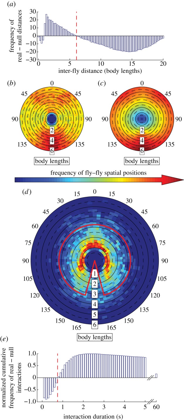
Establishing Canton-S males' interaction space based on repeated spatial–temporal behaviour. This figure presents an illustration of the method using the entire dataset of Canton-S males (n = 43). (a) The social distance is identified per group based on the large over-representation of close fly–fly distances in ‘real’ compared to ‘null’ data (see the electronic supplementary material, figure S1). The red dotted line indicates the social distance cut-off (see electronic supplementary material). (b–c) The angle and distance between each fly and all other flies' centre of mass is established for (b) all trials and (c) 500 ‘null’ trials (see electronic supplementary material). Numbers around heatmaps indicate angle. (d) The normalized frequency from the ‘null’ dataset is subtracted from the normalized frequency of the ‘real’ dataset, which reveals spatial positions seen more often in our assay than one would expect from non-social organisms. The angle and distance that captures the majority of this over-representation is established and plotted in red (see the electronic supplementary material). (e) Using the angle and distance criteria from (d), we count the number of interactions that last at least a specified time duration. The normalized histogram of ‘null’ data subtracted from the histogram of ‘real’ data is plotted, and the first positive time bin (red dotted line) indicates the time duration for which the putative interactions occur more often in the ‘real’ data.

When normalized ‘real’-‘null’ frequencies do not generate positive values it is classified as a ‘failed estimate’, which reveals a tendency to interact randomly. We established 95% confidence intervals (CIs) of social distance and interaction distance/angle/time by bootstrapping (15 trials chosen 500 times, each time creating a new ‘null’ dataset of the 15 trials). These bootstrapped estimates were also used in the principal component analysis (PCA; figure 2). We note that the estimates are dependent on the sample size, and expand as sample size increases (electronic supplementary material, figure S2). While the theoretical minimal sample size is 12 (to create ‘null’ datasets without overlap), the minimal effective sample size appears to be 15 (electronic supplementary material, figure S2). We also observe that several trials may bias the overall estimate (see Canton-S (in the dark) electronic supplementary material, figure S7, which generates a social space at the high end of the CI; table 1), and recommend the bootstrap approach to obtain a median (with at least 250 estimates; electronic supplementary material, figure S3).

Figure 2.

PCA of the interaction criteria. Our bootstrapped estimates were used to perform a PCA to determine whether these treatments generated interaction values that grouped in a multivariate sense. (a) Score for all treatments and coefficients of the variables. (b–f) Highlight specific comparisons within (a). (b) Overlap of strains and sexes. (c) Clustering of Canton-S and Canton-S in the dark. (d) Separation of scores for Canton-S, iav¹/Canton-S, and iav¹. (e) Separation of Canton-S, Orco²/Canton-S and Orco². (f) Overlap between poxn^ΔM22-B5SuperA-158 and poxn^ΔXBs6 (when the latter generates valid criteria).

Table 1.

Interaction criteria generated per genotype and sex. Each genotype's median social distance and their interaction criteria values are listed (95% CIs in parentheses). Failed estimates do not generate valid criteria. The difference in mean number of interactions per trial captured by these criteria versus the criteria used in [6] is indicated (Δ Interactions). The cited figures can be viewed in the electronic supplementary material.

strain	social space (body lengths)	interaction criteria			failed estimates (%)	Δ interactions	figure
		distance (body lengths)	angle (°)	time (s)
Canton-S ♀	6.25 (4.75–10.00)	2.50 (2.00–3.00)	160 (145–170)	0.6 (0.5–0.8)	0	3629	S4
Canton-S ♂	5.50 (3.75–9.00)	2.50 (2.00–3.25)	155 (130–175)	0.6 (0.4–1.0)	0	2924	1
Oregon-R ♀	6.25 (4.50–10.00)	2.50 (2.00–3.75)	155 (145–170)	0.6 (0.5–0.8)	0	3818	S5
Oregon-R ♂	4.00 (3.00–6.00)	1.75 (1.25–2.75)	115 (60–155)	0.4 (0.3–0.7)	0	1507	S6
Canton-S (dark)	5.50 (3.00–9.25)	2.25 (1.50–3.50)	135 (70–160)	0.4 (0.3–0.7)	0	2500	S7
iav1/Canton-S	3.50 (2.25–6.50)	1.75 (1.25–2.75)	135 (40–145)	0.4 (0.2–0.6)	0	1263	S8
iav1	4.75 (3.50–7.75)	3.00 (2.00–3.75)	125 (105–145)	1.1 (0.6–1.5)	0	1382	S9
Orco2/Canton-S	4.75 (3.25–7.00)	1.75 (1.50–3.00)	125 (65–150)	0.5 (0.3–1.3)	0	1014	S10
Orco2	2.50 (1.75–3.25)	1.75 (1.50–1.75)	90 (50–115)	1.0 (0.5–4.7)	33.4	660	S11
poxn ΔM22-B5SuperA-158	3.75 (2.50–5.75)	1.75 (1.25–2.25)	105 (10–135)	0.8 (0.2–1.3)	5.8	107	S12
poxn ΔXBs6	2.50 (1.50–3.50)	1.50 (1.25–1.75)	95 (55–115)	0.6 (0.4–0.9)	80.4	39	S13

4. Results and discussion

Each genotype generates a unique social interaction space in our arena, and our method is much more effective than previous approaches at detecting interactions (table 1). The generated interaction definitions agree subjectively with visual inspection when an interaction occurs (electronic supplementary material, movie S1) and fails to occur (electronic supplementary material, movie S2). The regulation of distance/angle when flies avoid interactions (electronic supplementary material, movie S2) suggests an active choice to either interact or abstain from interacting.

Group-based differences in patterns of behavioural interaction can be compared in two ways: treating each variable by itself (table 1), or accounting for potential multivariate aspects (PCA; figure 2). We see no distinct clustering along the PCA axes and the CIs of all variables overlap among strain and sex (figure 2b and table 1), and visual cues (figure 2c and table 1). Auditory treatments show clustering within the PCA separate from controls (figure 2d), yet all variables have overlapping CIs (table 1), which illustrates a multivariate aspect of interaction values. Unlike Simon et al. [4], our analysis method detected a significantly close social distance phenotype in olfactory-deficient mutants Orco² compared to its controls (non-overlapping CIs; table 1). In addition to a close social distance, the interaction space of these homozygous mutants appears disrupted (to visual inspection) with a discontinuous pattern between the antennae (electronic supplementary material, figure S11D versus figure 1d and electronic supplementary material, figure S10D) and show limited evidence of actively regulating interaction duration frequencies (electronic supplementary material figure S11E versus figure 1e and electronic supplementary material, figure S10E). This suggests that there is no clear characteristic time at which Orco² ‘interacted’, as opposed to crossed paths with another fly, which is revealed in its failure rate (33.4%; table 1). Similarly, visual inspection reveals that the gustatory-deficient mutant, poxn^ΔXBs6 [8] has a disrupted interaction space similar to Orco² (electronic supplementary material, figure S13D versus figure S12D), and a much higher ‘failure rate’ (80.4%). Surprisingly, when poxn^ΔXBs6 does generate valid criteria, it is almost indistinguishable from its control poxn^ΔM22-B5SuperA-158 (figure 2f and table 1).

The close social space, visually different distributions and the propensity for interactions of any duration to occur less than randomly expected (in both poxn^ΔXBs6 and Orco²; electronic supplementary material, figures S13E and S11E) suggests that both taste and smell are required for social spacing and interaction behaviours (table 1). An alternative hypothesis is that the indeterminate nature of the interactions is due to the sedentary movement of the mutants (electronic supplementary material, figure S14). However, poxn^ΔM22-B5SuperA-158 demonstrates similarly low movement yet generates valid criteria in 95% of the cases, indicating that this is a sufficient amount of locomotion for interactive behaviour in Drosophila.

When studying groups of social organisms, quantifying an interaction as a set of pre-defined values is done extensively, both implicitly and explicitly [1]. But this ignores the difference between the regulation and expression of an interaction. Our method quantifies the treatment-specific interaction space in systems with continuous tracking. This improvement helps overcome current limitations in evaluating similarities and differences in interactions across treatments, strains and even species. With this, we can start investigating the social regulation across phylogenies, and ultimately begin identifying the conserved features of social groups.

Data accessibility

Data deposited in the Dryad repository: http://doi.org/10.5061/dryad.5nv17.

Funding statement

This work was funded by grants to J. D. Levine from the Canadian Institutes for Health Research, National Sciences and Engineering Research Council of Canada, and Canada Research Chair.

References

- 1.Croft DP, James R, Krause J. 2008. Exploring animal social networks. Princeton, NJ: Princeton University Press. [Google Scholar]
- 2.Dankert H, Wang L, Hoopfer ED, Anderson DJ, Perona P. 2009. Automated monitoring and analysis of social behavior in Drosophila. Nat. Methods 6, 297–303. ( 10.1038/nmeth.1310) [DOI] [PMC free article] [PubMed] [Google Scholar]
- 3.Kabra M, Robie AA, Rivera-Alba M, Branson S, Branson K. 2013. JAABA: interactive machine learning for automatic annotation of animal behavior. Nat. Methods 10, 64–67. ( 10.1038/nmeth.2281) [DOI] [PubMed] [Google Scholar]
- 4.Simon AF, Chou MT, Salazar ED, Nicholson T, Saini N, Metchev S, Krantz DE. 2012. A simple assay to study social behavior in Drosophila: measurement of social space within a group. Genes Brain Behav. 11, 243–252. ( 10.1111/j.1601-183X.2011.00740.x) [DOI] [PMC free article] [PubMed] [Google Scholar]
- 5.Schneider J, Atallah J, Levine JD. 2012. One, two, and many--a perspective on what groups of Drosophila melanogaster can tell us about social dynamics. Adv. Genet. 77, 59–78. ( 10.1016/B978-0-12-387687-4.00003-9) [DOI] [PubMed] [Google Scholar]
- 6.Schneider J, Dickinson MH, Levine JD. 2012. Social structures depend on innate determinants and chemosensory processing in Drosophila. Proc. Natl Acad. Sci. USA 109(Suppl. 2), 17 174–17 179. ( 10.1073/pnas.1121252109) [DOI] [PMC free article] [PubMed] [Google Scholar]
- 7.Branson K, Robie AA, Bender J, Perona P, Dickinson MH. 2009. High-throughput ethomics in large groups of Drosophila. Nat. Methods 6, 451–457. ( 10.1038/nmeth.1328) [DOI] [PMC free article] [PubMed] [Google Scholar]
- 8.Boll W, Noll M. 2002. The Drosophila Pox neuro gene: control of male courtship behavior and fertility as revealed by a complete dissection of all enhancers. Development 129, 5667–5681. ( 10.1242/dev.00157) [DOI] [PubMed] [Google Scholar]
Associated Data
This section collects any data citations, data availability statements, or supplementary materials included in this article.
Supplementary Materials
Data Availability Statement