Image reconstruction: an overview for clinicians

Abstract

Image reconstruction plays a critical role in the clinical use of magnetic resonance imaging. The MRI raw data is not acquired in image space and the role of the image reconstruction process is to transform the acquired raw data into images that can be interpreted clinically. This process involves multiple signal processing steps that each have an impact on the image quality. This review explains the basic terminology used for describing and quantifying image quality in terms of signal to noise ratio and point spread function. In this context, several commonly used image reconstruction components are discussed. The image reconstruction components covered include noise pre-whitening for phased array data acquisition, interpolation needed to reconstruct square pixels, raw data filtering for reducing Gibbs ringing artifacts, Fourier transforms connecting the raw data with image space, and phased array coil combination. The treatment of phased array coils includes a general explanation of parallel imaging as a coil combination technique. The review is aimed at readers with no signal processing experience and should enable them to understand what role basic image reconstruction steps play in the formation of clinical images and how the resulting image quality is described.

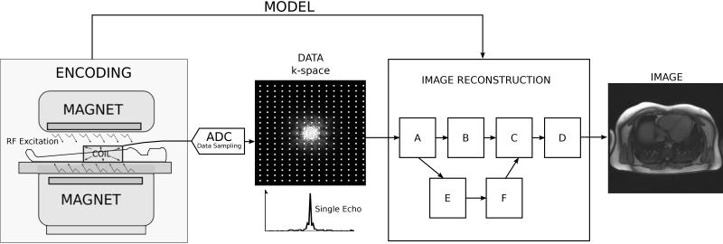
Magnetic resonance imaging (MRI) data are not acquired directly in image space. A set of data processing steps are required to turn the acquired raw data into actual images that can be interpreted by a clinician. The process of transforming the acquired raw data to images is called image reconstruction and on modern MRI devices, it is carried out by dedicated reconstruction software. A basic MRI acquisition (1) and the role of the image reconstruction process is illustrated in Fig. 1. The magnet with gradients and radiofrequency hardware serves as an encoding device. Radiofrequency radiation is transmitted into the patient where it excites the tissue magnetization and radiofrequency signals are emitted from the tissues. A radiofrequency coil is used to receive a superposition (sum) of all the tissue signals. Using magnetic gradient hardware, it is possible to create a spatially varying phase across the tissue signals and thus create different superpositions. This signal is digitized using an analog to digital converter (ADC) and the digitized form of the signal is usually referred to as raw data or k-space (2-5) data. Each data point in k-space represents a different superposition of the tissue signals. The image reconstruction software processes the k-space data to yield reconstructed images. During the transformation of the data, the reconstruction process relies on a description of actual gradient manipulations that took place during the measurement. This description is referred to as a data acquisition or encoding model and it is used to determine the appropriate signal processing steps. This model is based on assumptions about the data encoding process but the model may deviate from the actual encoding process due to imperfections in the measurement system. Most reconstruction processes consist of several steps (in Fig. 1 these are arbitrarily labeled A-F) that each impacts the quality of the final reconstructed images. The individual steps in the reconstruction process can be thought of as reconstruction building blocks. Several of the building blocks are common to many reconstruction processes and some are dedicated for specific applications. The aim of this review paper is twofold: First, to define basic criteria for characterizing the reconstructed image quality; Second, to review several basic reconstruction building blocks that are common to many applications and to provide an intuitive understanding of how these building blocks affect the quality of the final image.

Figure 1.

The role of the reconstruction process in the MRI measurement. The MRI hardware with radiofrequency transmit/receive system and spatial encoding gradients serves as the image encoding device. The actual measurement produces encoded imaging data (k-space), which is transformed by the image reconstruction process into images. The task of the image reconstruction process is to use information (a model) about the performed encoding steps to transform the data into images. The reconstruction process consists of multiple signal processing steps that are frequently depicted as steps in a reconstruction pipeline; here the steps are enumerated A-F.

Image Quality

Before describing specific image reconstruction algorithms and the signal processing steps they employ, it is important to establish basic tools and terminology for characterizing the quality of the reconstructed image. The term image quality is not meant to signify that one images is better than another. It is used broadly here to mean any characteristics that discriminate one image reconstruction result from another. There are many ways to characterize image reconstruction results. In this paper we will adopt the somewhat simplified view that there are three different categories of image characteristics: a) signal-to-noise ratio (SNR), b) pixel shape (point spread function), and c) artifacts. In the following sections, these three categories will be defined and described.

Signal To Noise Ratio (SNR)

All MRI measurements are affected by thermal noise (6, 7). In the bandwidth relevant to the MRI measurement, the spectrum of this noise is white (i.e. the noise level is not frequency dependent) and the amplitude distribution is Gaussian. The noise can be thought of as an additional random signal with mean value of zero and with a certain standard deviation. Consequently, we can characterize this noise in terms of this standard deviation, which is often denoted σ (Greek letter sigma). Said more plainly, the sampled MRI raw data consists of two components: signal and noise. As the data passes through the steps of the reconstruction process, both the signal and the noise are subjected to the same processing steps and finally both signal and noise are mapped to each individual pixel in the image. In each pixel the impact of the noise on the image quality is expressed in terms of the Signal to Noise Ratio or SNR (8, 9), which is defined as:

$$SNR(x,y)=\frac{S(x,y)}{\sigma (x,y)}$$ [1]

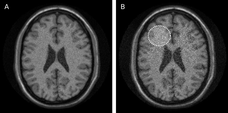
where S(x,y) is the signal intensity in a given pixel at location (x,y) and (x,y) is the standard deviation of the noise in that same pixel. Clearly, the SNR is not constant across the image. It varies both with the actual signal intensity and with the noise standard deviation. In some image reconstructions, the noise standard deviation is constant across the images, but the signal intensity is never really constant, and consequently signal to noise varies from tissue to tissue even if the noise distribution is the same in all pixels. An example of reconstruction results with different SNR levels is shown in Fig 2. The images in Fig. 2 and other neuro imaging examples were generated using the BrainWeb Simulated Brain Database (10). The image on the left (A) has better overall SNR than the image on the right (B). The image on the right also has spatially varying noise level. The region indicated by the dotted circle has higher noise level (and thus lower SNR) than other regions of the image.

Figure 2.

Illustration of reconstructions with different signal to noise ratio (SNR). Image A has higher overall SNR than image B. Furthermore, image B shows varying SNR levels in different image regions. The dotted circle illustrates an area with elevated noise and thus lower SNR.

There are several ways of evaluating the SNR in a specific image acquisition and reconstruction. The most intuitive way is to simply repeat the measurement (and reconstruction) a large number of times. This assumes that the signal remains constant from measurement to measurement and the only variation is caused by noise. The SNR in each pixel is then determined as the mean signal divided by the standard deviation across all the repetitions. Although this approach is conceptually simple, it is generally very hard to perform such measurements, especially in vivo where physiological changes and motion may contribute to an apparent increase in standard deviation (and thus a lower SNR). A more reliable and direct measure of the noise standard deviation is obtained using the pseudo replica method (11). This method relies on multiple reconstructions of the same data with new noise added to the data on each repetition. The characteristics of this added noise (amplitude and correlation between receive channels) are determined in a separate measurement where only noise is collected. After repeating the reconstruction multiple times, the standard deviation due to noise is determined as the standard deviation across all the replica reconstructions. The main advantage of this technique is that it works for any type of reconstruction (Cartesian, non-Cartesian, direct, iterative, etc.) but it is time consuming to repeat the reconstruction. Alternative methods that require fewer replicas have also been proposed (12), but they rely on local averaging in the image to improve the precision of the standard deviation estimates and they may not give reliable results when analyzing signal to noise in images where the noise may be correlated between pixels (13). For most Cartesian reconstructions, it is also possible to obtain an estimate of the signal to noise directly during the reconstruction by performing a reconstruction in units of SNR (14, 15).

Point Spread Function

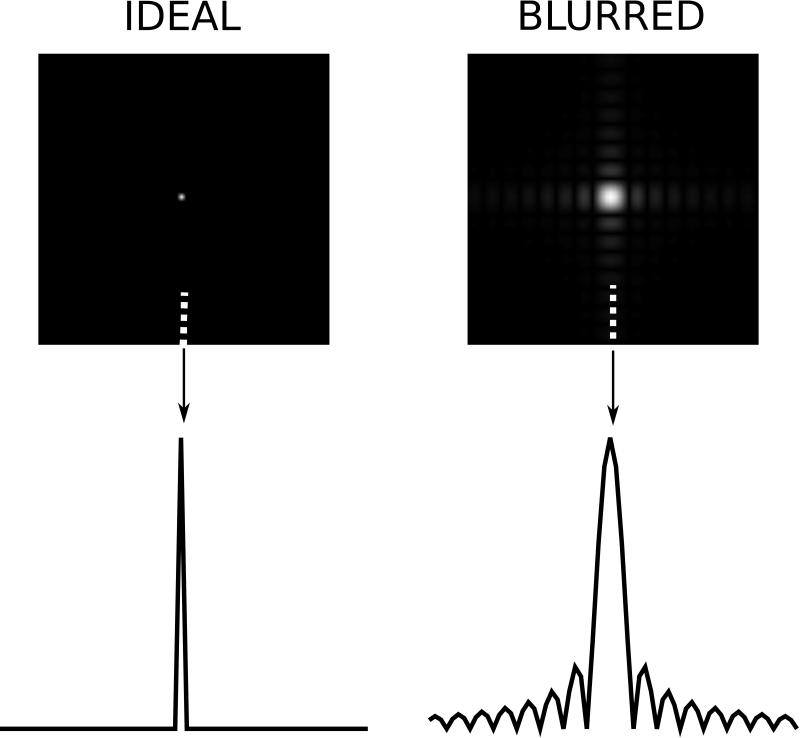
An important characteristic of an image is the point spread function, which is a useful way of characterizing how much neighboring pixels bleed into each other as a result of compromised spatial resolution and other effects. The PSF is the image that one would get if an object with a single point had been imaged. With an ideal point spread function, an image of a point source would be an image with signal only in a single pixel. However, typical point spread functions in MRI deviate significantly from this idealized form. A basic illustration of what a PSF looks like is seen in Fig. 3. The left column shows an idealized PSF from a simulated measurement with an in principle infinite spatial resolution image of an object with a single point source of tissue signal. Such a measurement can never be performed in practice but is included here to illustrate that the resulting image would have a single pixel with signal in it. On the right is shown the result of a measurement where the spatial resolution is reduced in both x and y directions. There are two main features to note in this PSF on the right. Firstly, the central peak of the PSF is broader than a single pixel. The interpretation of that is that neighboring pixels share information or signal will bleed from one pixel to another. This is the cause of blurry edges in images. It is difficult to determine exactly where an edge is when the point spread function causes that edge to be spread across multiple pixels. The second noticeable feature of the PSF is that it has more than one lobe, i.e. in addition to the (broadened) main lobe there are multiple side lobes. These side lobes are caused by truncation of the data space (k-space). Since we always sample a limited region of k-space, the PSF will always have such side lobes that cause ringing artifacts in the reconstructed images. This phenomenon is also known as Gibbs ringing (16, 17).

Figure 3.

Illustration of point spread functions. The two images on the top row show reconstruction results of simulated data from a numerical phantom with a single point source of signal. The image on the left shows an idealized scenario where all frequency components of the object are captured and the point source results in a single bright pixel. The image on the right was obtained with a simulated acquisition, which had lower spatial resolution. The lower row shows a plot of a single column of the point spread function for the column indicated by the arrow and dotted line.

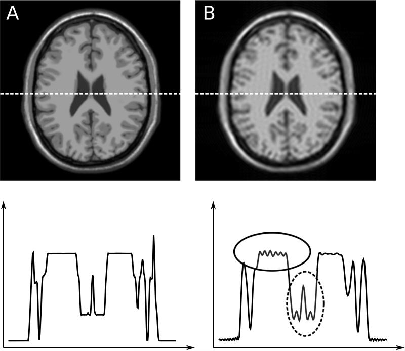
Figure 4 shows the effect that the PSFs in Fig. 3 would have on an image. On the left, the idealized measurement is shown for comparison purposes and on the right, the image affected by the PSF in Fig. 3B is shown. Effectively the image in Fig. 4B is obtained by through a convolution of the image in Fig. 4A with the PSF in Fig. 3B. The resulting image shows marked loss of spatial resolution (blurring), i.e. narrow structures that occupy only a single or a few pixels in the idealized image are now spread over more pixels. Furthermore, there is Gibbs ringing due to the truncation of k-space. As discussed later in this review, this ringing can be mitigated to some extend with raw data filters albeit at the expense of some loss of spatial resolution, i.e. a broadening of the PSF.

Figure 4.

Illustration of point spread function effect on simulated neuro images. The image on the left (A) has a simulated point spread function similar to A in Fig. 3. The image on the right (B) is affected by point spread function B of Fig 3. The plots on the bottom row show signal intensity plots corresponding to the row of pixels indicated by the dotted lines in the images. The image on the right appears blurred and exhibits Gibbs ringing. Note how the narrow structure in the central part is blurred out in image B as indicated by the dashed circle. Also note the clear Gibbs ringing artifacts indicated by the solid circle.

Artifacts

In the context of this review, artifacts occur whenever signals are erroneously assigned to pixels where they do not belong or when signal is absent or reduced in pixels where it should be present. In general this occurs when there is a discrepancy between the encoding model (see Fig. 1) and the encoding that actually took place. There is some fluid transition between artifacts and effects on the point spread function. As an example, Gibbs ringing could be considered an artifact or a change in PSF; in this review it has, somewhat arbitrarily, been designated as a PSF effect.

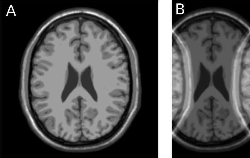
One of the most commonly occurring artifacts is aliasing or fold-over artifact. This artifact occurs when the field of view is set too small and signal from outside the field of view is assigned to pixels where it does not belong. An illustration of aliasing is seen in Figure 5. The image on the right (B) was acquired with half the field of view of the image on the left (A). In the model used in the reconstruction, it is assumed that there are no signal sources outside the field of view. In this case, the assumption is wrong and the result is an artifact.

Figure 5.

Illustration of aliasing or fold over artifact. The image on the right (B) was acquired with half the field of view of the image on the left (A). Signal outside the field of view is erroneously assigned to pixels within the field of view.

Other artifacts occur because unintended magnetic fields are present during the encoding or due to imperfections in the gradient hardware that cause delays or distortions of the gradient waveforms such that there is a mismatch between the expected encoding (the model) and the actual encoding. Delays and gradient distortions are common, but some acquisition types such as echo planar imaging (18), spiral imaging (19), or radial imaging (20, 21) are more susceptible to artifacts caused by gradient imperfections. Many of the artifacts can be corrected if the actual gradient waveforms are measured using dedicated sequences (22, 23) or specialized hardware (24).

There are numerous other hardware and patient related sources of artifacts and we refer the readers to general reviews on this topic (25, 26) or possibly reviews focused on specific applications, e.g. cardiac imaging (27).

The Reconstruction Task

The role of the reconstruction process is outlined in Fig. 1. In this section, a more formal description of the reconstruction task will be outlined to enable discussion of the specific components of this task. As indicated in Fig. 1, an encoding model is used to describe the encoding process that takes place in the imaging instrument. In practice, this encoding model is a mathematical description of how the nuclear magnetic resonance (NMR) signal is formed and how the spatial location information is encoded into this signal. This model is sometimes referred to as the forward model, since it describes the forward transformation from object signal to kspace data. Mathematically it can be written as:

$$E\rho =\mathbf{m}$$ [2]

where E is matrix which describes the encoding process, ρ is a vector containing the object signal intensities, and m is a vector containing the measured data. The object ρ is the unknown in the measurement. The matrix description is commonly used in the reconstruction literature. A different way of writing the same thing is that we apply some function, E( ), to the object and obtain the data:

$$\mathrm{E}\left(\rho \right(x,y\left)\right)=\mathrm{m}({\mathrm{k}}_x,{\mathrm{k}}_y)$$ [3]

Both descriptions are equivalent, but the most of the reconstruction literature uses the matrix description in Eq. 2 and it is used in the limited mathematical descriptions in this paper.

All that is known after the measurement is the measured k-space data (m) and some assumptions about the encoding, which are captured in the matrix E. The main task of the reconstruction is to recover a representation of the object ρ. Mathematically this is straightforward to describe as the inversion of Eq. 2:

$$\rho ={\mathbf{E}}^{-1}\mathbf{m}$$ [4]

In the same way that E is a mathematical description of the forward model, E⁻¹ is a mathematical description of the inverse model. For the purposes of this review, the exact details of the composition of these matrices need not be known; they merely serve as an abstract description of the process of transforming object to data and data to object.

The primary task of the reconstruction process is to perform the operations described in Eq. 4. This can either be done by finding a direct solution to Eq. 3 (a direct inverse) or by finding some approximate solution to the equation, possibly through an iterative reconstruction scheme. Direct application of the inverse model may in some cases lead to undesirable results (e.g. Gibbs ringing as described above) and thus the reconstruction may be modified to produce a result that is not exactly the inverse of the forward model but rather some modified result with more desirable features. In the following sections, basic methods for applying the inverse model will be discussed and several common reconstruction elements will be reviewed to explain their specific affects on the reconstruction result.

Direct and Iterative Reconstruction

There are several methods for finding the image reconstruction solution (Eq. 4). Some of these methods solve for the image directly and others arrive at an approximate image solution through a series of iterations. An example of a commonly used tool for direct reconstruction is the Fast Fourier Transform (FFT). The FFT is described in a bit more detail in a later section. More advanced acquisitions, e.g. studies employing parallel imaging (28-30), can also be reconstructed directly as outlined later in this review. In general, direct reconstruction is possible when the reconstruction problem can be broken into pure FFTs followed or preceded by solution of numerically smaller problems. The typical workflow for direct reconstruction is outlined in Fig. 6. In the direct approach, the encoding model is inverted in the reconstruction process and the data passes through a single set of operations to yield an image.

Figure 6.

Basic workflow for direct reconstruction. The object is subjected to an encoding process and a description of this encoding is captured in a model, which is forwarded to the reconstruction process. The reconstruction process inverts the forward model directly and applies the inverse model on the data to obtain the image result.

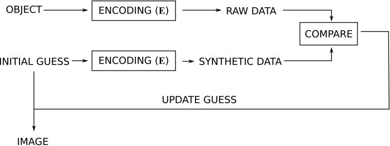
There are other types of reconstruction problems where direct solution is not possible or not practical. In general, this is the case when the reconstruction problem cannot be broken down into FFTs and other numerically small operations. In more mathematical terms these problems occur when the structure of the encoding matrix E is such that applying the inverse of E cannot be accomplished within a reasonable computation time. Examples of such problems are non-Cartesian parallel imaging (31) or some of the more modern non-linear reconstruction approaches, e.g. compressed sensing (32, 33). Although there are several different iterative reconstruction algorithms such as conjugate gradient (34), LSQR (35), non-linear conjugate gradient and others, they can conceptually be thought of as the algorithmic workflow outlined in Fig. 7. Instead of inverting the encoding model directly, as outlined in Fig. 6, the iterative methods try to guess what the solution would look like. This guess is then passed through the forward model, effectively subjecting it to the model encoding process to produce a kind of simulated raw data. This simulated raw data is then compared to the actual acquired raw data. If the simulated raw data and the acquired raw data are similar in some well defined sense (the residual is small), then the guess is assumed to be an adequate solution to the reconstruction problem. If they are not similar, the discrepancy between the simulated and the actual raw data can be used to update the guess in some way and repeat the process iteratively until the difference between simulated and acquired raw data is sufficiently small.

Figure 7.

Basic workflow for iterative reconstruction. Compared to the direct reconstruction in Fig. 6, the inverse model is never explicitly applied to the data. Instead, an initial guess of what the image could look like is made. This guess could be that all pixels are zero. The guess is subjected to the forward model and synthetic raw data is generated. This synthetic raw data is then compared to the actual acquired data and the difference (residual) is used to update the guess and the process is repeated until the difference between acquired and synthetic data is sufficiently small.

Iterative reconstruction algorithms tend to be slower than direct reconstruction algorithms. While this can be explained, to some extend, by the repetitive nature of the iterative algorithms, it is more commonly because the iterative algorithms are used to solve more complex reconstruction problems and the iterative approach is in fact a very efficient way of solving the problem. Fast implementations using graphics processors (GPUs) have been used to accelerated some iterative parallel imaging algorithms (36).

Cartesian and non-Cartesian Data

The most commonly used sampling strategies collect data on a rectilinear grid in k-space. More specifically, data is acquired line by line using what is know as Cartesian sampling. There is no fundamental reason why data should be acquired on a rectilinear grid and several non-Cartesian sampling strategies such as radial also known as projection imaging (20, 21) or spiral (19) k-space sampling are also frequently used. There are, however, many advantages to Cartesian sampling. The reconstruction of Cartesian data is simplified because the Fast Fourier Transform (see below) can be applied directly to the data and parallel imaging reconstruction often reduces to a set of smaller problems that are numerically easier to solve. Non-Cartesian data needs to be proceesed by a non-Cartesian Fourier transform, which is generally more computationally demanding as described below. Cartesian sampling is also more robust to acquisition system imperfections such as gradient distortions. Since such imperfections affect each line in k-space in the same way, the resulting artifacts tend to be more benign, whereas non-Cartesian acquisitions can suffer greatly from gradient imperfections. Non-Cartesian sampling is more challenging, but does provide some advantages for specific applications. Many non-Cartesian sampling strategies provide some oversampling of the center of k-space, which can be an advantage for dynamic imaging or in the case of accelerated imaging, the often fully sampled k-space can be used to extract calibration data for coil sensitivity or motion estimation (36, 37).

In this review, we make no specific distinction between Cartesian and non-Cartesian sampling as the general principles apply to both sampling schemes. However, most of the reconstruction steps discussed are more computationally demanding for non-Cartesian data and reconstruction times would be longer.

Reconstruction Components

Typical reconstruction programs used in clinical MRI systems are split into multiple components, which add specific qualities and features to the reconstruction process itself and the reconstructed images. It is beyond the scope of this review to cover all of them but in this section we will give a brief overview of some of the most common ones. A subsequent section will then give an example of a functioning reconstruction pipeline using these common components.

Fourier Transform

Magnetic resonance imaging data is acquired in the spatial frequency domain (units of [m⁻¹]) known as k-space. The k-space is related to the image domain (units of [m]) through a Fourier transform (38), which is analogous to the relation between temporal frequency (units [s⁻¹] or [Hz]) and time (units [s]). When samples are on a Cartesian grid, this Fourier transform can be computed very efficiently using the Fast Fourier Transform or FFT (39). The acronym FFT has now come to mean a category of algorithms for efficient calculation of the Fourier transform. The FFT operates on data that are on a Cartesian grid, but some applications using sampling patterns that deviate from a rectilinear grid, such as the original projection imaging technique (20, 21) or spiral imaging (19). In such cases, a non-uniform FFT is needed. A commonly used implementation of the non-uniform FFT in MRI reconstruction is the gridding algorithm (40). Efficient implementations can be found for both CPU (41, 42) and GPU (43, 44).

Noise Pre-Whitening

Clinical MRI data is commonly acquired with phased array coils, i.e. receive coils with multiple individual coil elements. The data from each coil element provide parts of the information needed to reconstruct the images and each coil element also contributes to the measurement noise, which ultimately propagates to the reconstructed images. The distribution of this noise between the coil elements has an impact on the quality (the SNR) of the reconstructed images. Specifically, if the noise level in one or a few of the coil elements is much higher than in others, that noise could end up dominating the reconstruction result. It also compromises the quality of the reconstruction if the noise between certain coil elements is correlated. Noise can be thought of as random perturbations of the data with a certain statistical distribution. The noise in a given coil element can be correlated with the noise in another coil element if the coils are coupled to each other such that they end up sampling the same noise to some extend. The noise distribution in the receive channels is often described with the noise covariance matrix (45), which is an N_coilsx N_coils matrix, which expresses the correlation between all possible pairs of coil elements. For a hypothetical 3-element coil, the matrix would be composed as:

$$\Sigma =\left[\begin{array}{ccc}\hfill \langle {\eta }_1\ast {\eta }_1^H\rangle \hfill & \hfill \langle {\eta }_1\ast {\eta }_2^H\rangle \hfill & \hfill \langle {\eta }_1\ast {\eta }_3^H\rangle \hfill \\ \hfill \langle {\eta }_2\ast {\eta }_1^H\rangle \hfill & \hfill \langle {\eta }_2\ast {\eta }_2^H\rangle \hfill & \hfill \langle {\eta }_2\ast {\eta }_3^H\rangle \hfill \\ \hfill \langle {\eta }_3\ast {\eta }_1^H\rangle \hfill & \hfill \langle {\eta }_3\ast {\eta }_2^H\rangle \hfill & \hfill \langle {\eta }_3\ast {\eta }_3^H\rangle \hfill \end{array}\right]$$ [5]

Where $\langle {\eta }_1\ast {\eta }_1^H\rangle$ is the expected value of the noise in coil 1 multiplied with the complex conjugate of the noise in coil 1 averaged over many instances of the same measurement, $\langle {\eta }_1\ast {\eta }_2^H\rangle$ is the same, but for the product of the noise in coils 1 and 2. The noise covariance matrix is a practical tool to immediately inspect the noise distribution in a given measurement system. By inspecting the 3-coil example structure in Eq. 5, we see that the diagonal elements are actually the noise variances (σ²) of each coils element and the off diagonal elements express how much correlation there is between coil elements. Statistically, the best reconstruction result is obtained when the noise covariance matrix is the identity matrix, i.e. a matrix with ‘1’ along the diagonal and ‘0’ on all off diagonal elements. That means that each coil element has the same noise level and the noise is not correlated between coil elements. In that condition, we say that the noise is white.

In practice, the noise covariance matrix is not the identity matrix, but before doing any reconstruction, it is possible to change the noise distribution by creating a set of virtual coils in which the noise is white. To accomplish this, it is common practice to measure the noise distribution before the actual measurement. The noise distribution is easily measured by performing a measurement in which the flip angle is zero or by simply turning on sampling in the receive channels without doing any excitation. The sampled noise can then be analyzed and an estimate of the noise covariance matrix is obtained. Once the noise covariance is known, it is possible to construct a matrix, which will decorrelate the noise such that the distribution is white. This step is commonly known as noise decorrelation or noise pre-whitening.

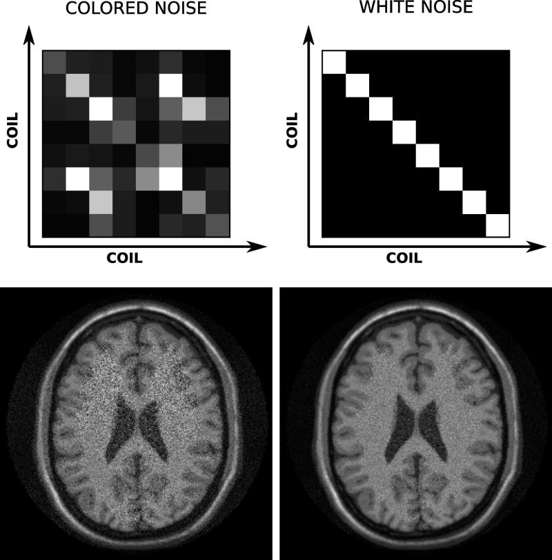
The effects of noise pre-whitening can be dramatic in some cases, especially if there are coil elements that have very different noise levels. Large differences in noise levels can be caused by broken coil elements or pre-amplifiers, and an inspection of the noise covariance matrix is often used as a quality assurance tool. Figure 8 shows an example of noise covariance matrices and the corresponding reconstruction results in a simulated brain MRI dataset. On the left of the figure, the noise covariance matrix of the 8-element array shows significant differences in noise levels between the coil elements and also some significant correlation between the elements as indicated by the non-zero off-diagonal elements. The reconstruction result displayed in the lower left shows increased noise in certain regions of the image. After noise pre-whitening the noise covariance matrix is identity (top right of Fig. 8) and the reconstruction result has improved SNR. It is important to note that these reconstruction results were obtained with exactly the same raw data, but a noise pre-whitening step was included in the reconstruction on the right of Fig. 8.

Figure 8.

Example of noise pre-whitening in a simulated neuro case. On the top left is a graphical rendering of the coil noise covariance matrix in the case where the noise levels are different in each channel and there is also some significant correlation between certain coil elements as indicated by the off diagonal elements. A direct reconstruction with this noise distribution yields the image on the lower left. The right hand side of the figure shows the results after noise pre-whitening. Now the effective noise covariance matrix is the identity matrix and the image shows marked improvement in the SNR.

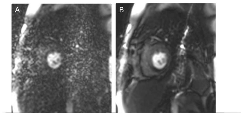
Figure 9 shows an in vivo cardiac perfusion study example. The image on the left (A) was reconstructed without noise pre-whitening, but due to a broken pre-amplifier in a single element of a 32-channel cardiac coil, the reconstruction result was dominated by the noise of that single element and images were non-diagnostic. By including a noise pre-whitening step, the images were dramatically improved as seen on the right (B) of Fig. 9. In this particular example noise pre-whitening changed a study from non-diagnostic to diagnostic. With a properly functioning coil, the improvement from noise pre-whitening is not as dramatic, but it generally improves SNR and it is considered good practice to perform noise pre-whitening when reconstructing data from phased array coils.

Figure 9.

An in vivo example of the effects of noise pre-whitening. On the left (A) is seen a direct reconstruction without pre-whitening in a case where a single coil element pre-amplifier was defective and added noise to the measurement. The images were non-diagnostic without the pre-whitening. After pre-whitening, the defective coil element was attenuated and the images were diagnostic.

Raw Data Filters

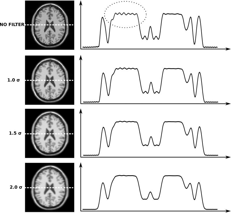
As discussed in the section on point spread function above, MR images can suffer from Gibbs ringing artifacts due to fact that only a limited region of k-space is sampled. These Gibbs ringing artifacts can create misleading artifacts, especially in situations where very bright signal regions border low signal regions and the bright signal rings into the lower signal areas. To mitigate this problem, a raw data filter is often applied. These raw data filters generally attenuate the signal at the outer part of k-space to create a more smooth transition between the sampled part of k-space and the edge of k-space. Since the outer regions of k-space are attenuated, the raw filters also causes a broadening of the point spread function, i.e. a loss in spatial resolution and an increase in SNR. Numerous different window shapes are commonly used on clinical MRI systems. Some of the more popular ones are the Hamming window and the Gaussian window. It is beyond the scope of this review to enumerate and analyze them all, but a comprehensive review of window shapes can be found in ref. (46).

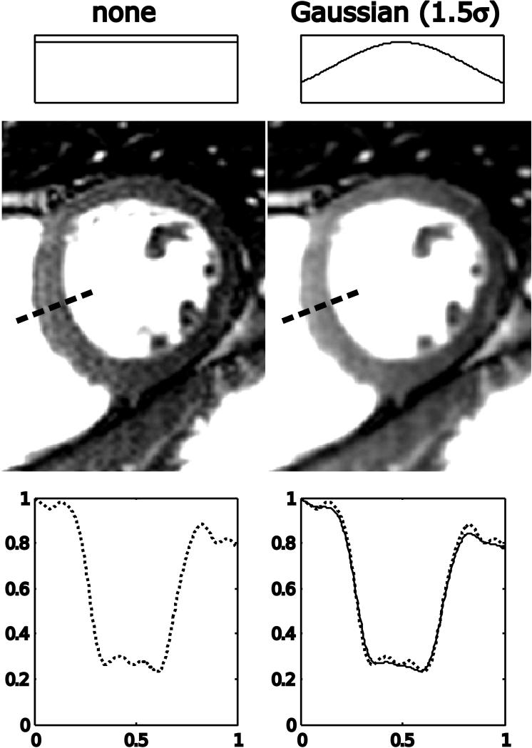
Figure 10 shows effects of raw data filtering on the example previously reviewed in Fig. 4. The top row demonstrates that a reconstruction without a raw data filter shows significant Gibbs ringing artifact and progressively more attenuation of the outer parts of k-space dampens the ringing at the expense of some loss of spatial resolution. Notice particularly the reduction of the ringing indicated by the dotted circle in the unfiltered case. Also notice how the central peak in the image is broadened and attenuated as the point spread function broadens. Figure 11 demonstrates the effect in an in vivo cardiac imaging case. Without the filtering, the bright blood pool causes Gibbs ringing seen as fluctuating signal pattern in the low signal intensity interventricular septum. After filtering, the signal intensity in the interventricular septum is much more uniform. This is also confirmed by inspection of the plots through the septum.

Figure 10.

Illustration of effects of raw data filtering on simulated neuro images. The top row is equivalent to the image in Fig. 4B, which was affected by the point spread function in Fig. 3B. There is considerable Gibbs ringing artifact highlighted by the dotted circle. The three bottom rows represent three different raw filters. The raw filters are all Gaussian shapes where the edge of the window has been set at 1.0, 1.5, and 2.0 times σ. Notice how the filters are progressively better at attenuating the Gibbs ringing albeit at the expense of a broadening of the point spread function.

Figure 11.

In vivo cardiac example of raw data filtering. The image on the left is reconstructed with no raw data filtering and there is evidence of Gibbs ringing artifacts in the interventricular septum as highlighted by the plot in the lower part of the figure. After filtering with a Gaussian filter with the edge of k-space set at 1.5* σ, the Gibbs ringing artifact is reduced. In the plot on the bottom right, the unfiltered profile through the interventricular septum is plotted with a dotted line and the filtered profile with a solid line.

Interpolation

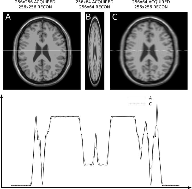
Magnetic resonance images are reconstructed with square pixels, i.e. a given pixel in the image represents the same distance in both x and y directions. However, the actual spatial resolution may vary among the spatial dimensions. Since there is a time penalty associated with acquiring more data in the phase encoding dimension, it is common to have a lower spatial resolution in the phase encoding direction. This is illustrated in Fig. 12. In practice, an acquisition with a matrix size of 256x256 might actually acquire 192 lines of k-space (75% phase resolution), each with 256 samples. If that acquired data is inserted into a 256x192 and simply Fourier transformed to image space to form a 256x192 image, the image would appear distorted, and the pixels would no longer be square. To reconstruct with square pixels, the 192 k-space lines are inserted into a 256x256 k-space matrix, where the 192 lines occupy lines 33-224 and the lines above and below this range are set to zero. After Fourier transform, the pixels will be square, but the resolution in the phase encoding direction is lower. Another way to express this is to say that although the pixels represent the same spatial distance in all directions (square or isotropic pixels), the point spread function is broader along the phase encoding dimension.

Figure 12.

Illustration of anisotropic resolution in a simulated neuro dataset. A) Full resolution image acquired with 256x256 samples in k-space and reconstructed on a 256x256 matrix. B) 256x64 (25% phase resolution) acquisition reconstructed on a 256x64 matrix. C) 256x64 acquisition reconstructed on a 256x256 matrix. A Gaussian raw data filter with 1.5*σ width was used in the phase encoding direction. The plot on the bottom depicts line plots in the horizontal direction; image A is represented with a solid line and image C with a dotted line. Notice the reduced resolution (blurring) in the phase encoding direction of image C.

Partial Fourier imaging (47-50) is a special case of reducing k-space encoding coverage to save scan time. In partial Fourier imaging, the reduction of k-space coverage is one sided and the reconstruction relies on symmetries in k-space to recover the missing data. This may cause some minor artifacts or a mild broadening of the point spread function, but it is not as severe as symmetric reduction in k-space coverage would cause. Due to the assumptions made during the reconstruction, the phase information in the resulting image may also be compromised.

Surface Coil Combination

Modern clinical MRI systems employ phased array coils (45, 51) to improve SNR in the reconstructed images and to enable parallel imaging acceleration of the acquisition process. This section briefly reviews how images from multiple coils are combined and how parallel imaging reconstruction can be viewed as a coil combination procedure.

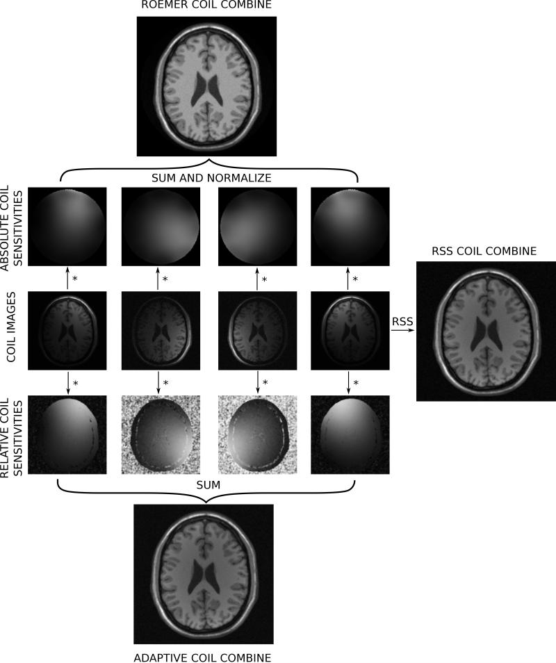
During the image reconstruction, k-space data is collected for each receive channel. The Fourier transform to image space produces an image for each receive channel and each of these images will be shaded slightly differently due to the spatially varying sensitivities of the receive coils. This is illustrated in Fig. 13, where the central row shows example coil images from a simulated acquisition with multiple coils. Notice how some coils show more signal in the front of the image and some show more signal in the back. The role of surface coil combination is to turn all these coil images into a single image. One of the simplest procedures for coil combination is the root-sum-squares (RSS) coil combination. With this technique, the magnitude of the combined image is found as the square root of the sum of the squared magnitudes of each coil image. The RSS coil combined image is shown on the right of Fig. 13. In the case of high SNR, this combination method is close to optimal (52) but the phase information is lost which is problematic for applications such as phase contrast flow (53) or phase sensitive inversion recovery reconstruction (54). The optimal coil combination when the coil sensitivities are know was outlined by Roemer et al. (45) and is found by multiplying the pixel value in each coil with the complex conjugate of the coil sensitivity for that channel, summing over all channels, and dividing this sum with the sum of the squared coil sensitivity in all channels. Effectively any phase added by the coil itself is removed and the signal is summed up. This is known as B1-weighted coil combination and is illustrated on in the top part of figure 13.

Figure 13.

Illustration of commonly used coil combination schemes. Four coil images are show in the central row of the figure. To the right of the coil image is an illustration of a simple but commonly used coil combination method; the root-sum-squares (RSS) coil combination. Above and below the coil images are two different sets of coil sensitivity maps. On the top, absolute coil sensitivities have been used to generate a B1-weighted coil combination with uniform intensity. On the bottom relative coil sensitivities have been used to generate an adaptively combined image.

Obtaining accurate estimates of coil sensitivities can be challenging. To obtain accurate information about both magnitude and phase of the coil sensitivities, it is necessary to perform a measurement where fully sampled images are acquired with both the surface coils and a homogeneous coil such as body coil typically used for excitation. Based on the ratio of signal in the two measurements accurate coil sensitivities can be obtained. However, this measurement is time consuming and the reconstructions that use the generated coil sensitivities are prone to artifacts if the patient moves. Consequently, coil sensitivities are often estimated with surface coil data only using a technique originally described by Walsh et al. (55). These coil sensitivities are known as relative coil sensitivities and are illustrated in the lower part of Fig. 13 along with the reconstruction result obtained with these sensitivities.

Both the RSS coil and the B1-weighted combination with relative sensitivities exhibit some signal intensity shading due to the fact that most of the coils have lower sensitivity in the center of the object and the center appears darker than the periphery. If accurate measurements of the coil sensitivities are done using both the surface coil elements and a body coil acquisition, this shading can be mitigated albeit at the expense of an increase in noise level in the central parts of the image. This is illustrated in the top part of Fig. 13.

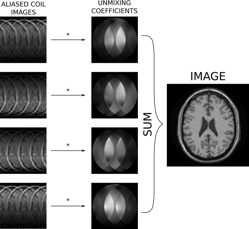
Parallel imaging (28-30, 56) is commonly used in many clinical applications to accelerate the acquisition. It is beyond the scope of this review to describe these methods in any detail, readers are referred to dedicated reviews on this topic, e.g. (57-60). Cartesian parallel imaging can be seen as a special case of coil combination where the role of the coil combination coefficients is to a) find the SNR optimal combination of the coils and b) remove any aliasing caused by undersampling. The coil combination coefficients can be found either in image space as it is done in SENSE reconstruction (29) or they can be found as a convolution matrix in k-space as it is done in GRAPPA reconstruction (30). In the latter case, the convolution matrix can be transformed to image space where it would also be a set of coil combination coefficients. In the case of parallel imaging, the coil combination coefficients are sometimes referred to as unmixing coefficients since their role is to unmix the aliased signals while combining the multi-coil data. This illustrated in Fig. 14, where a simulated case of parallel imaging with acceleration factor 4 is reconstructed using a set of unmixing coefficients obtained from coil sensitivities processed in a SENSE-type reconstruction.

Figure 14.

Illustration of coil combination in the case of parallel imaging with acceleration factor 4 in simulated neuro images. When parallel imaging is employed, a set of coil combination coefficients (unmixing coefficients) are estimated such that these coefficients a) remove the aliasing signal, and b) optimize the signal to noise.

Non-Cartesian parallel imaging represents a more complicated case, which is typically handled by iterative reconstruction algorithms as mentioned above. The readers are referred to some of the original publications, e.g. (31) or review papers covering this topic, e.g. (61).

Reconstruction Pipeline

The components that make up the steps in an MRI reconstruction program have been discussed above along with some of the criteria used to evaluate the impact on reconstruction quality that these steps have. The purpose of this section is to demonstrate how these components would be assembled to form a reconstruction pipeline. Most modern reconstruction software is designed as a pipeline processing system where the data passes through a set of steps before the final image is stored. Many of these steps are shared among different reconstruction schemes and some are unique to a specific application. Figure 15 is an illustration of a commonly used reconstruction pipeline for Cartesian parallel imaging. The first step in such a pipeline should be a pre-whitening step to mitigate the negative effects of noise correlation between surface coil elements. Next the data is inserted into a k-space array and filters are applied to reduce Gibbs ringing. Often image domain interpolation is done to reconstruct square pixels, this is achieved by zero-filling the outer parts of k-space. Finally the k-space datasets are transformed to image space, where the coils are combined. This coil combination could include parallel imaging as illustrated in Fig. 14.

Figure 15.

Illustration of a typical reconstruction pipeline for a Cartesian parallel imaging acquisition. The first step in the reconstruction is noise pre-whitening (noise adjust), which removes noise correlation in the data. The data pipeline then splits into two, one for the main image reconstruction and one for the processing of calibration data to form parallel imaging unmixing coefficients. The main processing pipeline performs raw data filtering, zero filling in k-space to ensure square pixels (image interpolation), Fourier transform, and finally coil combination using the parallel imaging unmixing coefficients. This final step turns the aliased channel images into a single combined image.

Discussion

The role of image reconstruction is to transform the acquired k-space data to images that can be interpreted clinically. The goal of this review was to give an introduction to the terminology used in image reconstruction and to discuss the commonly used reconstruction components in that context. There is no single authoritative text on MR image reconstruction, but a more in depth treatment of the subject can be found in text books on MRI, e.g. (62-64) and general signal processing text books (65) cover many of the topics such as filtering, Fourier transforms, and SNR. Additionally, there are several open source MR image reconstruction packages that can be used to find reference implementations and starting points when experimenting with image reconstruction, e.g. (44, 66, 67).

The reconstruction process involves multiple steps. Some of these steps are common to most reconstruction algorithms and others serve specialized functions for specific applications. This review has described some of the more commonly used components such as noise pre-whitening, filtering, Fourier transformation, and coil combination. Each step in the reconstruction has an impact on SNR and the point spread function in the final image. The processing steps may also introduce or mitigate reconstruction artifacts that could prevent correct interpretation of the images. Since the quality of the image (SNR, etc.) impacts the clinical usefulness of the MRI acquisition, it is important to have a working understanding of the basic terminology used to describe the image quality and to understand how the basic steps of the reconstruction might affect the final image quality. As an example, the Gibbs ringing phenomenon occurs frequently in clinical images and most clinical systems enable the user to control these artifacts by filtering of the raw data. Alternatively, the artifacts can be made smaller by increasing the spatial resolution.

The topics covered in this review have been focused on image reconstruction elements found in commonly used algorithms for 2D/3D Cartesian imaging. Time resolved imaging, e.g. cine cardiac MRI (68, 69), involve additional reconstruction elements such as sorting and binning of data into cardiac phases, and the additional data dimension provides an opportunity for data compression and accelerated acquisitions (70-74). Similarly, the added dimensions in flow imaging (75, 76) or parametric mapping (77, 78) can be exploited for acceleration using specialized reconstruction techniques. However, even the most sophisticated acquisition and reconstruction strategies will include some, if not all, of the image reconstruction components discussed in this review.

The take home message of this review is that image reconstruction can be broken down into a set of steps that the data passes through. Through careful analysis, it is possible to understand what impact each of the steps has on the image quality. The final image quality is determined by the combined effect of each processing step and can be described and quantified in terms of SNR, point spread function, and artifacts.

References

- 1.Hinshaw WS, Lent AH. An introduction to NMR imaging: From the Bloch equation to the imaging equation. Proc. IEEE. 1983;71:338–350. [Google Scholar]
- 2.Ljunggren S. A simple graphical representation of fourier-based imaging methods. J. Magn. Reson. 1983;54:338–343. [Google Scholar]
- 3.Twieg DB. The k-trajectory formulation of the NMR imaging process with applications in analysis and synthesis of imaging methods. Med. Phys. 1983;10:610–21. doi: 10.1118/1.595331. [DOI] [PubMed] [Google Scholar]
- 4.Hennig J. Review article K-space sampling strategies. Eur. Radiol. 1999;1031:1020–1031. doi: 10.1007/s003300050788. [DOI] [PubMed] [Google Scholar]
- 5.Pauly JM, Nishimura DG, Macovski A. Introduction to: A k-space analysis of small-tip-angle excitation. J. Magn. Reson. 2011;213:558–559. doi: 10.1016/j.jmr.2011.08.008. [DOI] [PubMed] [Google Scholar]
- 6.Johnson J. Thermal Agitation of Electricity in Conductors. Phys. Rev. 1928;32:97–109. [Google Scholar]
- 7.Nyquist H. Thermal Agitation of Electric Charge in Conductors. Phys. Rev. 1928;32:110–113. [Google Scholar]
- 8.Hoult D, Richards R. The signal-to-noise ratio of the nuclear magnetic resonance experiment. J. Magn. Reson. 1976;24:71–85. doi: 10.1016/j.jmr.2011.09.018. [DOI] [PubMed] [Google Scholar]
- 9.Edelstein WA, Glover GH, Hardy CJ, Redington RW. The intrinsic signal-to-noise ratio in NMR imaging. Magn. Reson. Med. 1986;3:604–618. doi: 10.1002/mrm.1910030413. [DOI] [PubMed] [Google Scholar]
- 10.Cocosco CA, Kollokian V, Kwan RK, Pike GB, Evans AC. BrainWeb: Online Interface to a 3D MRI Simulated Brain Database; 3rd International Conference on Functional Mapping of the Human Brain; 1996.p. 1996. [Google Scholar]
- 11.Robson PM, Grant AK, Madhuranthakam AJ, Lattanzi R, Sodickson DK, McKenzie CA. Comprehensive quantification of signal-to-noise ratio and g-factor for image-based and k-space-based parallel imaging reconstructions. Magn. Reson. Med. 2008;60:895–907. doi: 10.1002/mrm.21728. [DOI] [PMC free article] [PubMed] [Google Scholar]
- 12.Wiens CN, Kisch SJ, Willig-Onwuachi JD, McKenzie CA. Computationally rapid method of estimating signal-to-noise ratio for phased array image reconstructions. Magn. Reson. Med. 2011;66:1192–7. doi: 10.1002/mrm.22893. [DOI] [PubMed] [Google Scholar]
- 13.Hansen MS, Inati SJ, Kellman P. Noise propagation in region of interest measurements. Magn. Reson. Med. 2014:n/a–n/a. doi: 10.1002/mrm.25194. [DOI] [PMC free article] [PubMed] [Google Scholar]
- 14.Kellman P, McVeigh ER. Image reconstruction in SNR units: a general method for SNR measurement. Magn. Reson. Med. 2005;54:1439–47. doi: 10.1002/mrm.20713. [DOI] [PMC free article] [PubMed] [Google Scholar]
- 15.Kellman P, Erratum to, Kellman P, McVeigh ER. Image reconstruction in SNR units: a general method for SNR measurement. Magn Reson Med. 2005;54:1439–1447. doi: 10.1002/mrm.20713. Magn. Reson. Med. 2007;58:211-212. [DOI] [PMC free article] [PubMed] [Google Scholar]
- 16.Gibbs JW. Fourier’s Series. Nature. 1898;59:200–200. [Google Scholar]
- 17.Gibbs JW. Fourier’s Series. Nature. 1899;59:606–606. [Google Scholar]
- 18.Mansfield P. Multi-planar image formation using NMR spin echoes. J. Phys. C Solid State Phys. 1977;10:L55–L58. [Google Scholar]
- 19.Ahn CB, Kim JH, Cho ZH. High-speed spiral-scan echo planar NMR imaging-I. IEEE Trans. Med. Imaging. 1986;5:2–7. doi: 10.1109/TMI.1986.4307732. [DOI] [PubMed] [Google Scholar]
- 20.Lauterbur PC. Image Formation by Induced Local Interactions: Examples Employing Nuclear Magnetic Resonance. Nature. 1973;242:190–191. [PubMed] [Google Scholar]
- 21.Lauterbur PC, Lai C-M. Zeugmatography by Reconstruction from Projections. IEEE Trans. Nucl. Sci. 1980;27:1227–1231. [Google Scholar]
- 22.Duyn JH, Yang Y, Frank JA, van der Veen JW. Simple correction method for k-space trajectory deviations in MRI. J. Magn. Reson. 1998;132:150–153. doi: 10.1006/jmre.1998.1396. [DOI] [PubMed] [Google Scholar]
- 23.Mason GF, Harshbarger T, Hetherington HP, Zhang Y, Pohost GM, Twieg DB. A Method to measure arbitrary k-space trajectories for rapid MR imaging. Magn. Reson. Med. 1997;38:492–496. doi: 10.1002/mrm.1910380318. [DOI] [PubMed] [Google Scholar]
- 24.De Zanche N, Barmet C, Nordmeyer-Massner JA, Pruessmann KP. NMR probes for measuring magnetic fields and field dynamics in MR systems. Magn. Reson. Med. 2008;60:176–86. doi: 10.1002/mrm.21624. [DOI] [PubMed] [Google Scholar]
- 25.Henkelman RM, Bronskill J. Artifacts in Magnetic Resonance Imaging. Pergamon Press; 1987. [Google Scholar]
- 26.Morelli JN, Runge VM, Ai F, et al. An Image-based Approach to Understanding the Physics of MR Artifacts. RadioGraphics. 2011;31:849–866. doi: 10.1148/rg.313105115. [DOI] [PubMed] [Google Scholar]
- 27.Ferreira PF, Gatehouse PD, Mohiaddin RH, Firmin DN. Cardiovascular magnetic resonance artefacts. J. Cardiovasc. Magn. Reson. 2013;15:41. doi: 10.1186/1532-429X-15-41. [DOI] [PMC free article] [PubMed] [Google Scholar]
- 28.Sodickson DK, Manning WJ. Simultaneous acquisition of spatial harmonics (SMASH): fast imaging with radiofrequency coil arrays. Magn. Reson. Med. 1997;38:591–603. doi: 10.1002/mrm.1910380414. [DOI] [PubMed] [Google Scholar]
- 29.Pruessmann KP, Weiger M, Scheidegger MB, Boesiger P. SENSE: sensitivity encoding for fast MRI. Magn. Reson. Med. 1999;42:952–62. [PubMed] [Google Scholar]
- 30.Griswold MA, Jakob PM, Heidemann RM, et al. Generalized autocalibrating partially parallel acquisitions (GRAPPA) Magn. Reson. Med. 2002;47:1202–10. doi: 10.1002/mrm.10171. [DOI] [PubMed] [Google Scholar]
- 31.Pruessmann KP, Weiger M, Börnert P, Boesiger P. Advances in sensitivity encoding with arbitrary k-space trajectories. Magn. Reson. Med. 2001;46:638–51. doi: 10.1002/mrm.1241. [DOI] [PubMed] [Google Scholar]
- 32.Lustig M, Donoho D, Pauly JM. Sparse MRI: The application of compressed sensing for rapid MR imaging. Magn. Reson. Med. 2007;58:1182–1195. doi: 10.1002/mrm.21391. [DOI] [PubMed] [Google Scholar]
- 33.Lustig M, Donoho DL, Santos JM, Pauly JM. Compressed sensing MRI. Signal Process. Mag. IEEE. 2008;25:72–82. [Google Scholar]
- 34.Hestenes MR, Stiefel E. Methods of conjugate gradients for solving linear systems. J. Res. Natl. Bur. Stand. (1934) 1952;49:409. [Google Scholar]
- 35.Paige CC, Saunders MA. LSQR – An Algorithm for Sparse Linear-Equations and Sparse Least-Squares. ACM Trans. Math. Softw. 1982;8:43–71. [Google Scholar]
- 36.Sorensen TS, Atkinson D, Schaeffter T, Hansen MS. Real-time reconstruction of sensitivity encoded radial magnetic resonance imaging using a graphics processing unit. Med. Imaging, IEEE Trans. 2009;28:1974–1985. doi: 10.1109/TMI.2009.2027118. [DOI] [PubMed] [Google Scholar]
- 37.Hansen MS, Baltes C, Tsao J, Kozerke S, Pruessmann KP, Eggers H. k-t BLAST reconstruction from non-Cartesian k-t space sampling. Magn. Reson. Med. 2006;55:85–91. doi: 10.1002/mrm.20734. [DOI] [PubMed] [Google Scholar]
- 38.Bracewell R. McGraw-Hill Science/Engineering/Math. 3 edition 1999. The Fourier Transform & Its Applications; p. 640. [Google Scholar]
- 39.Cooley JW, Tukey JW. An algorithm for the machine calculation of complex Fourier series. Math. Comput. 1965;19:297–301. [Google Scholar]
- 40.Jackson JI, Meyer CH, Nishimura DG, Macovski A. Selection of a convolution function for Fourier inversion using gridding [computerised tomography application] IEEE Trans. Med. Imaging. 1991;10:473–8. doi: 10.1109/42.97598. [DOI] [PubMed] [Google Scholar]
- 41.Keiner J, Kunis S, Potts D. Using NFFT 3---A Software Library for Various Nonequispaced Fast Fourier Transforms. ACM Trans. Math. Softw. 2009;36:1–30. [Google Scholar]
- 42.Fessler JA, Sutton BP. Nonuniform Fast Fourier Transforms Using Min-Max Interpolation. IEEE Trans. Signal Process. 2003;51:560–574. [Google Scholar]
- 43.Sorensen TS, Schaeffter T, Noe KO, Hansen MS. Accelerating the nonequispaced fast Fourier transform on commodity graphics hardware. Med. Imaging, IEEE Trans. 2008;27:538–547. doi: 10.1109/TMI.2007.909834. [DOI] [PubMed] [Google Scholar]
- 44.Hansen MS, Sørensen TS. Gadgetron: An open source framework for medical image reconstruction. Magn. Reson. Med. 2012 doi: 10.1002/mrm.24389. [DOI] [PubMed] [Google Scholar]
- 45.Roemer PB, Edelstein WA, Hayes CE, Souza SP, Mueller OM. The NMR phased array. Magn. Reson. Med. 1990;16:192–225. doi: 10.1002/mrm.1910160203. [DOI] [PubMed] [Google Scholar]
- 46.Harris FJ. On the use of windows for harmonic analysis with the discrete Fourier transform. Proc. IEEE. 1978;66:51–83. [Google Scholar]
- 47.Margosian P, Schmitt F. Faster MR Imaging: Imaging with Half the Data. Heal. Care Instrum. 1986;1:195–197. [Google Scholar]
- 48.Cuppen J, van Est A. Reducing MR imaging time by one-sided reconstruction. Magn. Reson. Imaging. 1987;5:526–527. [Google Scholar]
- 49.Noll DC, Nishimura DG, Macovski A. Homodyne detection in magnetic resonance imaging. IEEE Trans. Med. Imaging. 1991;10:154–163. doi: 10.1109/42.79473. [DOI] [PubMed] [Google Scholar]
- 50.Liang Z-P, Boada FE, Constable RT, Haacke EM, Lauterbur PC, Smith MR. Constrained Reconstruction Methods in MR Imaging. Rev. Magn. Reson. Med. 1992;4:67–185. [Google Scholar]
- 51.Wright SM, Wald LL. Theory and application of array coils in MR spectroscopy. NMR Biomed. 1997;10:394–410. doi: 10.1002/(sici)1099-1492(199712)10:8<394::aid-nbm494>3.0.co;2-0. [DOI] [PubMed] [Google Scholar]
- 52.Larsson EG, Erdogmus D, Yan R, Principe JC, Fitzsimmons JR. SNR-optimality of sum-of-squares reconstruction for phased-array magnetic resonance imaging. J. Magn. Reson. 2003;163:121–123. doi: 10.1016/s1090-7807(03)00132-0. [DOI] [PubMed] [Google Scholar]
- 53.Pelc NJ, Sommer FG, Li KC, Brosnan TJ, Herfkens RJ, Enzmann DR. Quantitative magnetic resonance flow imaging. Magn. Reson. Q. 1994;10:125–47. [PubMed] [Google Scholar]
- 54.Kellman P, Arai AE, McVeigh ER, Aletras AH. Phase-sensitive inversion recovery for detecting myocardial infarction using gadolinium-delayed hyperenhancement. Magn. Reson. Med. 2002;47:372–83. doi: 10.1002/mrm.10051. [DOI] [PMC free article] [PubMed] [Google Scholar]
- 55.Walsh DO, Gmitro AF, Marcellin MW. Adaptive reconstruction of phased array MR imagery. Magn. Reson. Med. 2000;43:682–90. doi: 10.1002/(sici)1522-2594(200005)43:5<682::aid-mrm10>3.0.co;2-g. [DOI] [PubMed] [Google Scholar]
- 56.Griswold MA, Jakob PM, Nittka M, Goldfarb JW, Haase A. Partially parallel imaging with localized sensitivities (PILS) Magn. Reson. Med. 2000;44:602–9. doi: 10.1002/1522-2594(200010)44:4<602::aid-mrm14>3.0.co;2-5. [DOI] [PubMed] [Google Scholar]
- 57.Heidemann RM, Ozsarlak O, Parizel PM, et al. A brief review of parallel magnetic resonance imaging. Eur. Radiol. 2003;13:2323–37. doi: 10.1007/s00330-003-1992-7. [DOI] [PubMed] [Google Scholar]
- 58.Pruessmann KP. Encoding and reconstruction in parallel MRI. NMR Biomed. 2006;19:288–299. doi: 10.1002/nbm.1042. [DOI] [PubMed] [Google Scholar]
- 59.Larkman DJ, Nunes RG. Parallel magnetic resonance imaging. Phys. Med. Biol. 2007;52:R15–R55. doi: 10.1088/0031-9155/52/7/R01. [DOI] [PubMed] [Google Scholar]
- 60.Deshmane A, Gulani V, Griswold MA, Seiberlich N. Parallel MR imaging. J. Magn. Reson. Imaging. 2012;36:55–72. doi: 10.1002/jmri.23639. [DOI] [PMC free article] [PubMed] [Google Scholar]
- 61.Wright KL, Hamilton JI, Griswold MA, Gulani V, Seiberlich N. Non-Cartesian parallel imaging reconstruction. J. Magn. Reson. Imaging. 2014 doi: 10.1002/jmri.24521. [DOI] [PMC free article] [PubMed] [Google Scholar]
- 62.Haacke EM, Brown RW, Thompson MR, Venkatesan R. Magnetic Resonance Imaging: Physical Principles and Sequence Design. In: Wiley J, editor. Wiley-Liss; 1999. p. 914. [Google Scholar]
- 63.Liang Z-P, Lauterbur PC. Principles of Magnetic Resonance Imaging: A Signal Processing Perspective. IEEE Press. 2000 ISBN: 0-7803-4723-4. [Google Scholar]
- 64.Nishimura DG. Principles of magnetic resonance imaging. Stanford University; 1996. p. 223. [Google Scholar]
- 65.Oppenheim AV, Schafer RW, Buck JR. Discrete Time Signal Processing. 1999:870. [Google Scholar]
- 66.Fessler J. [Accessed April 7, 2014];Image reconstruction toolbox. Available at: http://web.eecs.umich.edu/~fessler/code/index.html.
- 67.Vahedipour K. [Accessed April 7, 2014];Codeare. Available at: http://www.codeare.org/
- 68.Lenz GW, Haacke EM, White RD. Retrospective cardiac gating: A review of technical aspects and future directions. Magn. Reson. Imaging. 1989;7:445–455. doi: 10.1016/0730-725x(89)90399-8. [DOI] [PubMed] [Google Scholar]
- 69.Carr JC, Simonetti O, Bundy J, Li D, Pereles S, Finn JP. Cine MR angiography of the heart with segmented true fast imaging with steady-state precession. Radiology. 2001;219:828–34. doi: 10.1148/radiology.219.3.r01jn44828. [DOI] [PubMed] [Google Scholar]
- 70.Riederer SJ, Tasciyan T, Farzaneh F, Lee JN, Wright RC, Herfkens RJ. MR fluoroscopy: Technical feasibility. Magn. Reson. Med. 1988;8:1–15. doi: 10.1002/mrm.1910080102. [DOI] [PubMed] [Google Scholar]
- 71.Van Vaals JJ, Brummer ME, Thomas Dixon WT, et al. “Keyhole” method for accelerating imaging of contrast agent uptake. J. Magn. Reson. Imaging. 1993;3:671–675. doi: 10.1002/jmri.1880030419. [DOI] [PubMed] [Google Scholar]
- 72.Kellman P, Epstein FH, McVeigh ER. Adaptive sensitivity encoding incorporating temporal filtering (TSENSE) Magn. Reson. Med. 2001;45:846–52. doi: 10.1002/mrm.1113. [DOI] [PubMed] [Google Scholar]
- 73.Tsao J, Boesiger P, Pruessmann KP. k-t BLAST and k-t SENSE: dynamic MRI with high frame rate exploiting spatiotemporal correlations. Magn. Reson. Med. 2003;50:1031–42. doi: 10.1002/mrm.10611. [DOI] [PubMed] [Google Scholar]
- 74.Breuer FA, Kellman P, Griswold MA, Jakob PM. Dynamic autocalibrated parallel imaging using temporal GRAPPA (TGRAPPA) Magn. Reson. Med. 2005;53:981–5. doi: 10.1002/mrm.20430. [DOI] [PubMed] [Google Scholar]
- 75.Hansen MS, Baltes C, Tsao J, et al. Accelerated dynamic Fourier velocity encoding by exploiting velocity-spatio-temporal correlations. Magn. Reson. Mater. Physics, Biol. Med. 2004;17:86–94. doi: 10.1007/s10334-004-0062-8. [DOI] [PubMed] [Google Scholar]
- 76.Baltes C, Kozerke S, Hansen MS, Pruessmann KP, Tsao J, Boesiger P. Accelerating cine phase-contrast flow measurements using k-t BLAST and k-t SENSE. Magn. Reson. Med. 2005;54:1430–1438. doi: 10.1002/mrm.20730. [DOI] [PubMed] [Google Scholar]
- 77.Doneva M, Börnert P, Eggers H, Stehning C, Sénégas J, Mertins A. Compressed sensing reconstruction for magnetic resonance parameter mapping. Magn. Reson. Med. 2010;64:1114–20. doi: 10.1002/mrm.22483. [DOI] [PubMed] [Google Scholar]
- 78.Velikina JV, Alexander AL, Samsonov A. Accelerating MR parameter mapping using sparsity-promoting regularization in parametric dimension. Magn. Reson. Med. 2013;70:1263–73. doi: 10.1002/mrm.24577. [DOI] [PMC free article] [PubMed] [Google Scholar]