Intrinsic multi-scale analysis: a multi-variate empirical mode decomposition framework

Abstract

A novel multi-scale approach for quantifying both inter- and intra-component dependence of a complex system is introduced. This is achieved using empirical mode decomposition (EMD), which, unlike conventional scale-estimation methods, obtains a set of scales reflecting the underlying oscillations at the intrinsic scale level. This enables the data-driven operation of several standard data-association measures (intrinsic correlation, intrinsic sample entropy (SE), intrinsic phase synchrony) and, at the same time, preserves the physical meaning of the analysis. The utility of multi-variate extensions of EMD is highlighted, both in terms of robust scale alignment between system components, a pre-requisite for inter-component measures, and in the estimation of feature relevance. We also illuminate that the properties of EMD scales can be used to decouple amplitude and phase information, a necessary step in order to accurately quantify signal dynamics through correlation and SE analysis which are otherwise not possible. Finally, the proposed multi-scale framework is applied to detect directionality, and higher order features such as coupling and regularity, in both synthetic and biological systems.

1. Introduction

Complex systems are governed by latent coupling mechanisms across multiple components; these couplings are typically exhibited at unique temporal and spatial scales. Examples can be found in biology, economics, engineering systems and climatology. A goal of this work is to understand and explain the fluctuating system dynamics based only on a few observed variables, which are often nonlinear and statistically non-stationary. This motivates the need for a comprehensive and unifying analysis framework, comprising inter- and intra-component measures, which operates at the multi-scale level.

A successful data analysis framework is critically dependent on the choice of data-scale representation, and its ability to provide reliable and robust data-association metrics for real-world data. To this end, it is necessary to consider scales which are: (i) physically meaningful—free from rigid mathematical constraints so as to accommodate a signal representation which matches closely our intuitive understanding of signal-generating mechanisms and (ii) data driven—in order to reflect the inherent fluctuations embedded in the data, without a priori knowledge. These requirements are desirable, for instance, when analysing neural systems via electroencephalography (EEG). It is well known that EEG is best represented at different temporal scales (e.g. delta, theta, alpha, beta and gamma bands), and a physically meaningful approach is required to cater for their inherently nonlinear statistics [1]. Furthermore, the properties of the scales can vary, their centre frequencies may be either fixed (e.g. steady-state responses or power-line interference) or drifting (the alpha rhythm can occupy the range 8–13 Hz), all suggesting the need for a data-driven approach.

These requirements for operation at an intrinsic scale level are not met by traditional scale-estimation methods: (i) Fourier-based measures are not reliable unless the data are stationary and (ii) the wavelet transform can better cater for real-world data scales, however its use is dependent on the correct choice of mother wavelet (not data-driven). Another problem common to all projection-based schemes (Fourier, wavelet) is the blurred representation arising from integral transforms, and the associated limitation by the Heisenberg uncertainty principle—increasing time resolution causes a decrease in frequency resolution, and vice versa. In addition, standard filtering operations are not adequate as they require a priori selection of the frequency ranges of interest, which can bias findings [2].

These shortcomings have motivated the empirical mode decomposition (EMD) algorithm [3], a recursive nonlinear filter which decomposes a time series into a set of narrow-band scales¹ known as intrinsic mode functions (IMFs). This makes possible the estimation of time-varying signal dynamics at each scale at the highest level of resolution—instantaneous frequency and instantaneous amplitude—via the Hilbert transform. The time–frequency features obtained from the IMFs can be represented by the Hilbert–Huang spectrogram (HHS) or, in its time-marginalized form, the marginalized Hilbert–Huang spectrum (MHHS). Unlike projection-based schemes or conventional filtering approaches, the scales obtained using EMD are physically meaningful (figure 1) and data driven (figure 2). The approach has been successfully employed in disciplines ranging from ocean engineering [5] to nuclear science [6]. Work on a rigorous mathematical basis for EMD is still ongoing and is supported by a vast number of empirical studies. A link with a standard multi-scale representation was established in [7,8], which illustrated the behaviour of EMD as a dyadic filterbank in the presence of white Gaussian noise (WGN). For a pair of narrow-band unmodulated components that are closely spaced in the spectrum, the EMD interpretation is a single amplitude-modulated component [9]—providing a more sparse and intuitive signal representation (heterodyning). Multi-variate extensions of EMD include the complex EMD [10], rotation-invariant EMD [11], bivariate (BEMD) [12], trivariate [13] and multi-variate (MEMD) algorithms [14], while for greater robustness and to enforce a dyadic filterbank structure, several noise-assisted EMD (NA-EMD) algorithms have been proposed, such as ensemble EMD (EEMD) [15] and noise-assisted MEMD (NA-MEMD) [16].

Figure 1.

Physically meaningful scales. The EMD decomposes a time series into narrow-band components (IMFs) which admit physically meaningful estimates of both instantaneous frequency and amplitude via the Hilbert transform. The time-domain waveform of an IMF with fixed frequency and modulated amplitude is shown in (a). The time–frequency spectrogram using standard Fourier theory (b) shows two uniform-amplitude components with uniform frequencies, while the representation using the Hilbert transform (c) yields a single frequency component with modulated amplitude—closely matching with intuition.

Figure 2.

Data-driven scales. The narrow-band concept underpinning EMD encompasses both components with uniform or fixed frequencies (i.e. sinusoids) and components with drifting frequencies (e.g. alpha rhythm in EEG). (a) The spectra of the first IMF (c₁) and the second IMF (c₂) obtained from the sum of a high-frequency uniform algorithms component and a low-frequency drifting algorithms component. (b) The spectra of the first IMF (c₁) and the second IMF (c₂) obtained from a signal comprising the sum of a high-frequency drifting algorithms component and a low-frequency uniform algorithms component. Observe that the spectral properties (centre frequency, bandwidth) of the scales obtained via EMD have automatically adapted to extract the underlying components in the data, not possible to achieve with conventional filters without a priori knowledge.

Approaches for characterizing intrinsic system dynamics using EMD can be categorized based on: (i) the type of EMD algorithm used (EMD, EEMD, MEMD, NA-MEMD); (ii) the data-association measure(s) used (correlation, coherence, etc.); (iii) the type of component dependence they model (inter- or intra-); and (iv) the domain in which they operate (IMF, HHS, MHHS). Table 1 provides an overview of some recently introduced multi-scale intrinsic measures.

Table 1.

A review of EMD-based approaches for intrinsic multi-scale analysis.

	EMD alg.	inter/intra	domain	measure
[3]	EMD	intra	IMF	inst. freq., inst. amp.
[7]	EMD	intra	IMF	energy density
[17]	EMD	inter	IMF	phase shift
[2]	EMD	inter	IMF	phase synchrony
[18]	EMD	intra	MHHS	spectral entropy
[19]	EMD	inter	IMF	partial directed coherence
[20]	EEMD	inter	IMF	intrinsic correlation
[21]	BEMD	inter	MHHS	asymmetry
[22]	MEMD	intra	IMF	multi-scale sample entropy
[23]	NA-MEMD	inter	HHS	coherence
[24]	EEMD	inter	IMF	coherence
			HHS	Granger causality

Intrinsic inter-component measures characterize the scale-wise system behaviour between the components. The multi-scale intrinsic correlation scheme in [20] proposed an adaptive sliding window based on the instantaneous frequencies of the IMFs, greatly enhancing the usefulness of correlation measures for non-stationary data. Also, the localized properties of EMD-based scales make them ideal for the estimation of phase, and the data-driven nature of such scales enables the modelling of drifting components. For instance, the EMD approach was instrumental in evaluating inter-dependencies in phase between blood pressure and blood volume flow after stroke [17]. More recently, phase synchrony (PS)—the temporal locking of phase information [25,26]—has been examined using univariate EMD [2], BEMD [27] and MEMD [28]. Compared with conventional bandpass filters, it was shown in [19] how EMD-based partial directed coherence—a measure for determining directionality in coupled outputs—better estimates inter-hemispheric features of patients with Parkinson's disease. An MHHS model for characterizing imagined motor actions has shown that asymmetry, a measure which characterizes the lateralization of amplitude information between two components, is more accurately extracted compared with approaches based on the Fourier spectrum [21]. More recent contributions include modelling coherence within the HHS domain via MEMD [23], and ways of estimating directionality with coherence and Granger causality within the IMF and HHS domains via EEMD [24].

Intrinsic intra-component measures characterize the scale-wise system behaviour within each component; typical examples include instantaneous frequency and instantaneous amplitude. Statistical significance tests, based on the dyadic filterbank property of EMD, have been developed to identify information-bearing scales [8], while Li et al. [18] calculated spectral entropy using the MHHS and found that it was better suited to tracking responses to anaesthesia in EEG than other spectral entropy measures. Sample entropy (SE) [29] and its multi-scale extension, multi-scale sample entropy (MSE) [30,31], are widely used tools for assessing complex nonlinear couplings within time series. The EMD has been used to enhance the SE operation: (i) by facilitating data conditioning by, for example, trend removal [32,33] and (ii) as a means for achieving data-driven multi-scale operation by replacing the conventional coarse-graining scales with data-adaptive scales via IMFs [22,34].

It is widely accepted that there are many advantages in processing phase and amplitude dynamics of complex systems separately [26] and not, for instance, combining both within a single measure (cross-correlation). Indeed, PS and asymmetry are, by design, restricted to considering only phase or amplitude, yet much of the existing EMD-based data-association metrics fail to fully exploit its properties to enable separate phase/amplitude characterization. Another problem is that many inter-component studies employ univariate EMD and ensemble EMD, however these algorithms cannot guarantee that IMFs from different measured variables will have sufficiently similar bandwidths to enable a rigorous and fair comparison.

The aim of this work is therefore threefold: (i) to consolidate the intrinsic multi-scale measures for multi-variate data; (ii) to introduce a novel class of inter-component measures, such as intrinsic correlation and intrinsic PS; and (iii) to introduce the intra-component measure intrinsic SE. We also emphasize the importance of either an MEMD or NA-MEMD approach to intrinsic scale analysis. These make possible the simultaneous decomposition of system components while ensuring a sufficient degree of bandwidth similarity between the scales—a prerequisite for inter-component analysis. We further illustrate advantages of the estimation of feature relevance in intrinsic PS through the multi-variate framework. The operation of SE for narrow-band data is illuminated through an intuitive model derived for a sinusoidal input—the narrow-band signal in its most basic form. We furthermore show that fully decoupling amplitude and phase information within the IMF domain improves the performance of correlation and SE in estimating component directionality and regularity. The proposed framework is validated over comprehensive case studies for both synthetic (Rössler) and biological (cardiac–respiratory, neural) systems.

2. Empirical mode decomposition

We next present a brief review of EMD and its multi-variate extensions.

(a). Univariate empirical mode decomposition

Unlike projection-based schemes (Fourier, wavelet) which trade time localization for frequency localization, or vice versa, the Hilbert transform can obtain a physically meaningful estimate of frequency at each time instant (instantaneous frequency) if the input signal satisfies monocomponent criteria [35]. In other words, the signal can be modelled by a single amplitude/frequency component changing slowly over time. A precise definition of the term ‘monocomponent’ does not exist, and a widely used approximation are the set of so-called narrow-band criteria [4]. These criteria primarily concern the global properties of the signal, that is, the number of extrema and the number of zero crossings should differ by at most one. In [3], an additional local criterion was proposed—that the mean of the two envelopes that interpolate the local maxima and local minima must be approximately zero. Signals that satisfy both the local and global criteria are called IMFs and enable an estimate of both instantaneous frequency and amplitude via the Hilbert transform; they can even exhibit nonlinear or non-stationary statistics. The univariate EMD [3] (see algorithm 1) embarks upon these criteria to decompose a single-channel input x into a set of IMFs, that is,

$$x(t)=\sum _{i=1}^M{c}_i(t),$$ 2.1

where the symbol t denotes the sample index and {c_i(t)}, i=1,…,M, denotes the set of IMFs.

The sifting process (steps (ii)–(v) in algorithm 1) is stopped once the signal detail $\hat{c}(t)$ satisfies the IMF criteria, the practical implementation of which has been addressed in a number of contributions [3,36,37]. In general, the more sifting operations that are performed, the more narrow-band the IMF spectra become. Care must be taken not to perform too many sifting operations as this can produce large numbers of IMFs with uniform amplitudes (i.e. components which approximate a Fourier basis)—contradicting the data-driven nature of the analysis.

(b). Multi-variate extensions of empirical mode decomposition

Bivariate [12] as well as multi-variate [14] extensions of the EMD algorithm have been proposed to extend its operation for any number of data channels. A key concept in creating these extensions has been the definition of the local mean for multi-variate data. The BEMD algorithm [12] proposed a solution for bivariate data wherein the data are projected in Q directions, with each direction vector defined based on equidistant points along the unit circle (uniform angular sampling; figure 3a). Univariate estimates of the envelope in each direction are averaged to give a bivariate envelope, the centre (e.g. barycentre) of which is the local mean. This concept was extended further in [14] for multi-variate data of dimension P—multi-variate EMD (MEMD)—wherein the projection of the data is performed for Q direction vectors, based on a pointset on a hypersphere generated using a low-discrepancy Hammersley sequence (figure 3b). Algorithm 2 describes the MEMD operation for a P-variate time series, with a pointset of size Q, giving the set of IMF components $c_i^p(t)$, where i denotes the IMF index (i=1,…,M) and p denotes the data channel index (p=1,…,P).

Figure 3.

Sampling directions for multi-variate extensions of EMD. (a) Projection set (Q) for bivariate EMD based on uniform angular sampling. (b) Projection set (Q) for multi-variate EMD based on a low-discrepancy Hammersley sequence.

3. Noise-assisted empirical mode decomposition algorithms

Performing inter-component measures via EMD requires the comparison of IMFs from different system components or outputs. To preserve the physical meaning of the analysis, it is desirable to compare IMFs that are similar, that is, IMFs with similar centre frequencies and bandwidths. However, standard forms of EMD are sensitive to local signal variations, meaning that signals with similar global statistics can yield IMFs which are different in number and bandwidth (problem of uniqueness [38]). Such problems are further illuminated by the phenomenon referred to as mode mixing, whereby modes with similar properties (frequencies) appear at different IMF levels.

Figure 4 shows the power spectral densities (PSDs) for IMFs of WGN, obtained using EMD, for different numbers of sifting operations.² Increasing the number of sifting operations enables control over the properties of the IMFs (mean frequency and bandwidth). Observe that using the standard EMD algorithm the averaged filterbank structure exhibits slower roll-off, as well as an increasing degree of overlap between the IMF spectra for an increased number of sifting operations. This indicates poor stability in the EMD operation; decompositions of signals with similar statistics can produce IMFs with varying spectral content.

Figure 4.

Averaged power spectral densities (PSDs) of the first four IMFs, obtained using EMD for WGN. (a) PSDs of IMFs for 15 sifting operations. (b) PSDs of IMFs for 1000 sifting operations. The degree of overlap between the IMF spectra indicates poor stability in the EMD operation; decompositions of signals with similar statistics can produce IMFs with different spectral content.

NA-EMD algorithms aim to help enforce a pre-defined structure within the IMFs by using noise as a decomposition reference. This has been shown to help alleviate the problems of uniqueness and mode mixing. To date, most research has focused on the use of WGN which, as discussed earlier, enforces a dyadic filterbank structure into its IMFs [7,8]. While this somewhat hinders the data-driven operation of EMD, it can be essential in multi-channel or multi-component operations where the requirement is to compare scales of similar frequencies.

(a). Ensemble empirical mode decomposition

In ensemble EMD (EEMD) WGN is added directly to the signal of interest before applying EMD. The approach creates a perturbation within the resulting IMF set, but through averaging same-index IMFs for a sufficiently large number of ensembles the effect of the added WGN is cancelled out. The perturbed signal is given by

$$x_v(t)=x(t)+v(t),$$ 3.1

where x(t) denotes the signal of interest and v(t) a realization of WGN. Algorithm 3 describes the EEMD operation. The influence of the noise is determined by the signal-to-noise ratio (SNR), that is, the ratio of powers of the input signal and the perturbation

$$10{\log }_{10}\frac{\sum _t{x}^2(t)}{\sum _t{v}^2(t)}.$$ 3.2

The operation of the EEMD algorithm for different SNRs is shown in figure 5; reducing the SNR improves the stability of the EEMD operation and reduces the degree of overlap between the IMF spectra.³ A problem with the EEMD algorithm, however, is that many noise realizations (S) are required for the IMF set to converge and for the effect of the added noise to be cancelled out. For low SNRs, the value of S can be prohibitively large.

Figure 5.

Averaged PSDs of the first four IMFs, obtained using EEMD for WGN. (a) PSDs of IMFs for 15 sifting operations with an SNR of 20 dB. (b) PSDs of IMFs for 15 sifting operations with an SNR of 2 dB. Reducing the SNR (increasing the power of the added noise) improves the stability in the operation and reduces the degree of overlap between the IMF spectra.

(b). Noise-assisted multi-variate empirical mode decomposition

The NA-MEMD algorithm was proposed in [16] to circumvent the problems associated with added noise in EEMD. Within NA-MEMD, WGN is not added to the signal directly but rather it is placed within separate channels adjoining the signal channels and—owing to the scale alignment property of MEMD—the noise channels enforce dyadic structure within the signal channels. In other words, unlike EEMD where the local mean is estimated for the perturbed signal and iteratively removed from the perturbed signal, in NA-MEMD the local mean is estimated from the perturbed signal but iteratively removed from the perturbation-free signal. As there is no direct perturbation to the signal—termed indirect perturbation—the output is always an IMF set with less residual noise than EEMD [39]. Algorithm 4 describes the operation of NA-MEMD.

Despite the difference in the NA-MEMD methodology (indirect perturbation), its operation can be controlled in a similar way to EEMD via the two key parameters: (i) the SNR of the perturbation and (ii) the number of independent noise channels.

(i). Noise-assisted multi-variate empirical mode decomposition: perturbation signal-to-noise ratio

As with the EEMD, increasing the power of the noise (reducing the SNR) imposes a more pronounced filterbank structure within the IMFs. In practice, the powers in each of the noise channels are identical, and the SNR is defined by the ratio of the kth signal channel and any of the noise channels

$$10{\log }_{10}\frac{\sum _t{(x^k)}^2(t)}{\sum _t{(v^i)}^2(t)},\mathrm{\forall }\hspace{0.17em}i\in P_v.$$ 3.3

Defining the SNR in this way, the total perturbation SNR will also depend on the number of noise channels. Assuming WGN and equal power in each of the noise channels, the total SNR can be written as follows:

$${\text{SNR}}_{\mathrm{T}}=\text{SNR}-10{\log }_{10}{P}_v,$$ 3.4

where P_v is the number of noise channels. Although the concept of SNR is similar for both algorithms, a direct comparison between NA-MEMD and EEMD for the same perturbation SNR cannot be made due to the differences in operation—indirect versus direct perturbation. Another reason is that, in the NA-MEMD estimation of the local mean, the perturbation of the signal is performed by linearly mixing the signal channels and the noise channels based on the Q direction vectors. The relative weighting between the noise and signal channels changes for each direction vector, and therefore each estimation of the local mean is an ensemble average for different perturbation SNRs. The NA-MEMD SNR parameter in equation (3.3) controls the range of these perturbation SNRs generated mid-operation.

(ii). Noise-assisted multi-variate empirical mode decomposition: number of independent noise channels

Recall that MEMD operates, at each sifting operation, by linearly mixing the signal channels and the noise channels based on the Q direction vectors—thus giving the perturbed signal in the context of NA-MEMD. The perturbation is therefore a linear mixture of the noise channels. For an increasing number of noise channels, the correlation between the perturbations will decrease. As the perturbations should ideally be as independent as possible between sifting operations for optimum noise-assisted performance, this implies that the number of noise channels should be as large as possible.

Figure 6 illustrates the link between the number of independent noise channels and the performance of NA-MEMD. Figure 6a shows the PSD of the IMFs obtained using NA-MEMD with a low noise power (SNR 41 dB) and 10 noise channels. The simulation was repeated but constraining the operation so that the noise vectors were identical in each channel (figure 6b). In this way, the perturbation SNR was identical in both figure 6a,b, and yet the decreased level of correlation between the perturbations has adversely affected the performance of NA-MEMD—the overlap between the IMF spectra is greater in figure 6b. In summary, the number of noise channels should be as large as possible—computation time permitting—to ensure optimum noise-assisted performance.

Figure 6.

Averaged PSDs of the first four IMFs obtained using NA-MEMD for WGN. Both panels were obtained with 15 sifting operations, with an SNR of 41 dB, and 10 noise channels, where (a) each of the noise vectors were different and (b) all the noise vectors were the same. Increasing the number of independent noise channels in NA-MEMD helps enforce the desired quasi-dyadic structure and reduces the degree of overlap between the IMF spectra.

(c). Mode alignment

The advantage of noise-assisted forms of EMD is that they enable a more reliable estimation of the IMFs by providing a decomposition reference. Nonetheless, even with some noise-assisted algorithms, phenomena such as mode mixing can still occur. Figure 7a(i) shows a time series comprising a 10 Hz and a 50 Hz sinusoid, and figure 7a(ii–iv) shows its decomposition using EEMD; figure 7a(v) shows a time series composed of the 10 Hz sinusoid only and figure 7a(vi–viii) shows its decomposition. Observe that mode mixing has occurred and the IMFs most closely related to the 10 Hz component are located at different IMF indices for the two decompositions (c₃ and c₄). When the two signals were decomposed simultaneously using NA-MEMD as a single bivariate signal (with 11 adjoined noise channels), figure 7b illustrates much better mode alignment. The most important aspect of an MEMD approach, via either standard MEMD or NA-MEMD, is that even if mode mixing occurs it is likely to happen simultaneously in each channel. In this way, multi-component comparisons at the IMF level are matched and physically meaningful.

Figure 7.

NA-EMD algorithms. (a) A signal comprising a 10 Hz and a 50 Hz sinusoid (x¹) (i), and its IMFs via EEMD (ii–iv), and a signal comprising a 10 Hz sinusoid (x²) (v), and its IMFs via EEMD (vi–viii). (b) The same signals were decomposed simultaneously using NA-MEMD. Observe significantly improved mode alignment using NA-MEMD.

(iii). Mode alignment simulation 1

We next provide a novel assessment of the mode-alignment property, whereby EEMD and NA-MEMD were applied to decompose two time series,

$$x^1(t)=\cos (2\pi f_{1}t)\text{and}{x}^2(t)=x^1(t)+\cos (2\pi f_{2}t),$$ 3.5

where the first signal, x¹, comprises a sinusoid with frequency f₁, and the second signal, x², is the summation of x¹ and another sinusoid with frequency f₂=kf₁ where k>2. Signal decompositions are said to be aligned if the IMFs containing f₁ are of the same IMF index.

Scenarios where the value of f₁ is between the centre frequencies of two consecutive IMF spectra are more likely to cause mode misalignment. Therefore, for completeness, we next vary f₁ by, at least, the full spectral range of a dyadic IMF (an IMF from a set of IMFs which exhibit a dyadic filterbank structure), and also vary f₂, by varying k, in a similar fashion. Instances of mode alignment between the two signals were determined for scenarios where the values of f₁ ranged from 10 to 25 Hz at intervals of 1 Hz, and the values of k ranged from 2.5 to 4 at intervals of 0.1. The sampling frequency was 1000 Hz and the signal duration was 1 s. The EEMD algorithm was applied to each signal with S=100 realizations and with added WGN of different⁴ SNRs: −20, −10, 0, 5, 10, 15 and 20 dB. In the case of NA-MEMD, the signals were decomposed as a single bivariate signal with four noise channels for different SNRs.

Figure 8 shows the number of instances of mode alignment for 30 realizations of the algorithms for each of the simulation parameters (f₁, k). Figure 8a shows the results obtained using NA-MEMD with SNR 0 dB, and Figure 8b–h shows the results obtained using EEMD for increasing SNR. The result in Figure 8a is representative of the results obtained using NA-MEMD for all other SNRs; the algorithm enabled mode alignment for all scenarios. In the case of the EEMD operation, owing to the iterative nature of EMD, the higher frequency component in x², that is, f₂, influenced the index at which the lower frequency component, that is, f₁, was located. This resulted in several instances of mode misalignment. Increasing the SNR of EEMD influenced its operation in two ways. Firstly, it changed the frequency of f₁ at which mode misalignment occurred; this is as expected as the IMF spectra will change for increasing levels of added noise, becoming increasingly dyadic. Secondly, increasing the SNR of EEMD somewhat increased the instances of mode alignment, but several cases were still found for SNRs as low as −20 dB; furthermore decreasing the SNR below −20 dB may require a computationally prohibitive increase in the number of WGN realizations (S) to cancel out the unwanted effects of the added noise.

Figure 8.

Mode-alignment property. The number of instances of mode alignment for the IMFs of x¹ and x² with different parameter values (f₁, k), see equation (3.6), obtained using (a) NA-MEMD with 0 dB SNR, (b) EEMD with −20 dB SNR, (c) EEMD with −10 dB SNR, (d) EEMD with 0 dB SNR, (e) EEMD with 5 dB SNR, (f) EEMD with 10 dB SNR, (g) EEMD with 15 dB SNR and (h) EEMD with 20 dB SNR.

(iv). Mode alignment simulation 2

As already discussed, noise-assisted algorithms hinder somewhat the data-driven operation of EMD by enforcing a filterbank structure. However, unlike the EEMD algorithm, NA-MEMD allows a trade-off between the noise-assisted and data-driven operations, particularly in the context of mode alignment. To illustrate this, consider the following sinusoids:

$$x^1(t)=\sin (2\pi f_{1}t)+v(t)\mathrm{and}{x}^2(t)=\sin (2\pi f_{1}kt)+v(t),$$ 3.6

where v is added WGN (independent realizations for each signal) and k is a scalar which defines the level of similarity in frequency between x¹ and x². For k=1, the signals are identical in frequency, and for k>1 the frequency of x² is greater than x¹, etc. The NA-MEMD algorithm (five noise channels, SNR of 0 dB) was applied to the signals separately, where f₁ was 100 Hz with a sampling frequency of 1000 Hz, the SNR induced by v was 20 dB and k=0.8. The information-bearing IMF for x¹, that is, the IMF containing the sinusoid, was located at IMF index 3. Figure 9a shows the c₃ component for the x¹ and x² operations; observe that there is no mode alignment. The NA-MEMD algorithm was applied again but by jointly decomposing x¹ and x² as a single multi-variate component; observe now that mode alignment is present. Figure 10 shows the number of instances of mode alignment for each of the simulation parameters (f₁,k) using separate a and joint b operations. It is seen that joint operations increase the number of mode-alignment instances; highlighting that NA-MEMD can sacrifice the dyadic structure to enable mode alignment based on the properties of the input (data driven).

Figure 9.

NA-MEMD adapts to facilitate mode alignment. The index 3 IMF obtained for x¹ (i) and x² (ii) using: (a) separate NA-MEMD operations and (b) a joint NA-MEMD operation. Through the joint operation, the dyadic filterbank restriction was alleviated so as to allow mode alignment between x¹ and x² (data-driven operation).

Figure 10.

NA-MEMD adapts to facilitate mode alignment. The number of instances of mode alignment within NA-MEMD with different parameter values (f₁,k), see equation (3.6), obtained using: (a) separate NA-MEMD operations and (b) joint NA-MEMD operations. The joint-operation approach increases the number of instances of mode alignment—highlighting the data-driven capabilities of NA-MEMD.

4. Intrinsic multi-scale analysis

We denote a single (P=1) or multi-channel IMF set (P>1) obtained via NA-MEMD by $c_i^p(t)$, where i denotes the IMF index (i=1,…,M) and p denotes the channel index (p=1,…,P). As the IMFs satisfy narrow-band criteria they admit the application of the Hilbert transform, defined by

$$\mathcal{H}\{c_i^p(t)\}=\frac{1}{\pi }{P}_{\mathrm{c}}{\int }_{-\mathrm{\infty }}^{\mathrm{\infty }}\frac{c_i^p(t^{\prime })}{t-t^{\prime }}\hspace{0.17em}\text{d}{t}^{\prime },$$ 4.1

where P_c is the Cauchy principal value. In this way, each IMF can be expressed as a complex analytic signal, formed from $c_i^p(t)$ and $\mathcal{H}\{c_i^p(t)\}$, giving

$$z_i^p(t)=c_i^p(t)+j\mathcal{H}\{c_i^p(t)\}=a_i^p(t)\hspace{0.17em}{\mathrm{e}}^{j{\theta }_i^p(t)},$$ 4.2

where the instantaneous amplitude, $a_i^p(t)$, and the instantaneous phase, ${\theta }_i^p(t)$, are given by

$$a_i^p(t)={[{(c_i^p(t))}^2+{(\mathcal{H}\{c_i^p(t)\})}^2]}^{1/2}\text{and}{\theta }_i^p(t)=\arctan \left(\frac{\mathcal{H}\{c_i^p(t)\}}{c_i^p(t)}\right).$$ 4.3

Instantaneous frequency can then be defined as the derivative of the instantaneous phase

$$f_i^p(t)=\frac{\text{d}{\theta }_i^p(t)}{\text{d}t}\frac{1}{2\pi }.$$ 4.4

Finally, we define the uniform-amplitude IMF (UA-IMF) set as

$${\hat{c}}_i^p(t)=\frac{c_i^p(t)}{a_i^p(t)},$$ 4.5

which is fully decoupled from amplitude information.

This gives us the opportunity to examine measures which can operate either at the IMF level or at the level of instantaneous amplitude or frequency. The considered measures in the next section are correlation and PS, which assess inter-channel dynamics, and SE, which reveals intra-component behaviour.

(a). Intrinsic correlation

The standard cross-correlation at the IMF level, between channels p₁ and p₂ at IMF index i and lag τ, is given by

$$r_c^{p_1,p_2}(i,\tau )=\frac{⟨(c_i^{p_1}(t)-{\overline{c}}_i^{p_1})(c_i^{p_2}(t-\tau )-{\overline{c}}_i^{p_2})⟩}{\sqrt{⟨{(c_i^{p_1}(t)-{\overline{c}}_i^{p_1})}^2⟩⟨{(c_i^{p_2}(t)-{\overline{c}}_i^{p_2})}^2⟩}},$$ 4.6

where the symbol 〈⋅〉 denotes averages over multiple time measurements, and $\overline{\cdot }$ denotes the sample mean. Additionally, the intrinsic scale nature of the IMFs makes possible the estimation of cross-correlation within the instantaneous amplitudes

$$r_a^{p_1,p_2}(i,\tau )=\frac{⟨(a_i^{p_1}(t)-{\overline{a}}_i^{p_1})(a_i^{p_2}(t-\tau )-{\overline{a}}_i^{p_2})⟩}{\sqrt{⟨{(a_i^{p_1}(t)-{\overline{a}}_i^{p_1})}^2⟩⟨{(a_i^{p_2}(t)-{\overline{a}}_i^{p_2})}^2⟩}}$$ 4.7

and instantaneous frequencies

$$r_f^{p_1,p_2}(i,\tau )=\frac{⟨(\hspace{0.17em}{f}_i^{p_1}(t)-{\overline{f}}_i^{p_1})(\hspace{0.17em}{f}_i^{p_2}(t-\tau )-{\overline{f}}_i^{p_2})⟩}{\sqrt{⟨{(\hspace{0.17em}{f}_i^{p_1}(t)-{\overline{f}}_i^{p_1})}^2⟩⟨{(\hspace{0.17em}{f}_i^{p_2}(t)-{\overline{f}}_i^{p_2})}^2⟩}}.$$ 4.8

The usefulness of such measures is illustrated in figure 11 for the example of two 1 Hz sinusoidal components, x¹ and x², of duration 10 s, with x² leading x¹ by (π/5) (0.1 s). Identical frequency modulations were induced within each component but at different time instants, (4−8) s in x¹ and (4.2−8.2) s in x² (figure 11a(i)). As each component satisfies IMF criteria, the instantaneous frequencies can be determined (figure 11a(ii)). Figure 11b(i) shows that the maximum cross-correlation between the time series occurs at lag 0.1 s. The positive nature of the delay lag indicates that x² leads x¹; however, the measure accounts only for the overall difference in phase and fails to cater for the frequency modulation. Figure 11b(ii) illustrates the advantage of considering cross-correlation of the instantaneous frequencies: a maximum value accurately occurs at a negative lag of −0.2 s, revealing that a modulation first occurred in x¹ and the true leading component of the system.

Figure 11.

Cross-correlation. (a) Two time series, x¹ and x² (i), and their instantaneous frequencies (ii). (b) The standard maximum correlation coefficient at the signal/IMF level occurs at 0.1 s (i), but the correct maximum correlation coefficient at the instantaneous frequency level occurs at −0.2 s (ii). Cross-correlation within the IMFs caters only for the overall phase difference, and fails to account for the periods of frequency modulation which occurred first in x¹.

(b). Intrinsic phase synchrony

One of the most widely used inter-component measures is PS, which characterizes the temporal locking of phase information. As already discussed, EMD is ideally suited to calculating PS as, unlike Fourier and wavelet methods, it enables the estimation of highly localized phase information and, unlike bandpass filter methods, it determines the relevant output oscillations in a data-driven manner so that synchrony events are unlikely to be missed.

To assess the degree of the PS between IMFs where the instantaneous phase difference is given by ϕ_i(t), deviation from perfect synchrony can be quantified by the phase synchrony index (PSI) [25]—see algorithm 5 for more details. The PSI ranges between 0 and 1, with 1 indicating perfect synchrony and 0 a non-synchronous state.

One of the challenges when calculating PS is in assessing its true statistical relevance. It is often the case that a level of PS will be detected even if there is no underlying phase locking present. Spurious PS events are more likely to be detected when the data are of limited length or if they are non-stationary [40]. Surrogate data are typically used to address this problem; random time series, which ideally retain all properties of the original signals except for phase locking, are generated and used to create PS confidence intervals. If the PS value estimated between the signals lies within the confidence intervals, it is likely to be spurious. In previous EMD-based PS studies, surrogates which preserve the power spectrum of the original data but which randomize their phase have been used. As noted in [2] and as illustrated in §3, the univariate EMD cannot guarantee that IMFs obtained from statistically similar signals will have similar bandwidths, thus compromising their value in creating confidence intervals. Although the EEMD algorithm enables greater consistency (dyadic structure) in the EMD operation, repeating the process for a large number of surrogates is not feasible (high computational complexity).

We here illustrate both the advantages of noise-assisted approaches and a means for assessing PS relevance via NA-MEMD. We consider the noise channels of the NA-MEMD process as surrogates with the same power spectrum as the inputs but with randomized phase. The PS is estimated within the signal channel pairs, and the confidence intervals at each IMF level are formed by assessing the PS between pairs of noise channels. For instance, an NA-MEMD operation with P_v noise channels gives P_v!/((P_v−2)!2!) surrogate pairs to determine confidence intervals. Consider a frequency-modulated signal described by

$$x(t)=\cos (2\pi f_{\mathrm{c}}t+h{\theta }_m(t)),$$ 4.11

where f_c is the carrier frequency, θ_m is a slowly varying random baseband signal, and h is a scalar (0≤h<1). Increasing h induces an increasing level of random frequency modulation, the degree of which can be assessed by $f_{\mathrm{\Delta }}=|f_{max}-f_{\mathrm{c}}|/f_{\mathrm{c}}$ where $f_{max}$ denotes the maximum frequency in x. If f_Δ<0.5, the signal will satisfy IMF criteria (narrow-band, dyadic). The NA-MEMD approach with surrogate noise channels was applied to assess PS from narrow-band frequency-modulated time series generated from the above model. The carrier frequency of each time series was 1 Hz, the sampling frequency was 100 Hz, and the time length was 5 s. A value for h was selected so as to induce a frequency modulation averaging f_Δ=0.3. The PS analysis was performed within overlapping windows of length 3 s. The number of noise channels was 11, giving 55 surrogate pairs to determine the PSI confidence intervals.

Figure 12a shows two different narrow-band time series with added WGN (SNR 10 dB), and figure 12b shows the PSI estimated using NA-MEMD. The confidence intervals here represent the mean PSI for the noise channels ±2 standard deviations. Observe that the PSI estimate for the signal is, at each IMF index, contained within the confidence intervals, indicating that any detected PS is likely to be spurious. Figure 12c shows identical narrow-band frequency-modulated time series generated from the model described in equation (4.9) with added WGN (SNR 10 dB, different realizations for each time series), in this way creating phase-locking at the frequency of x¹ and x² (approx. 1 Hz). This is reflected by the high level of PSI (≈1) at IMF index 6 (average instantaneous frequency 1 Hz) in figure 12d which lies far outside the confidence intervals.

Figure 12.

PS estimation using NA-MEMD. (a) Different narrow-band frequency-modulated time series with added WGN, x¹ and x², generated from the model described in equation (4.9). (b) The PSI estimated at different IMF indices for the signals in (a), with the value occurring within the confidence intervals obtained from the noise channels—indicating that it is not statistically significant (no synchronization). (c) Identical narrow-band frequency-modulated time series with added WGN, x¹ and x², generated from the model described in equation (4.9). (d) The PSI estimated at different IMF indices for the signals in (c), with the value occurring outside the confidence intervals at IMF index 6—indicating a statistically relevant estimate of synchronization.

(c). Intrinsic sample entropy

The entropy of a dynamical system describes its rate of information generation, and is a powerful metric for understanding complex systems. Motivated by the inadequacy of standard entropy measures for short and noisy time series, a class of techniques which measure signal regularity, known as approximate entropy [41], have been introduced. Sample entropy (SE) [29] is an extension of approximate entropy, which exhibits greater consistency across different signal lengths and parameters. The SE algorithm is described in algorithm 6; it characterizes the likelihood that similar patterns within a time series will remain similar when the pattern lengths are increased. In general, the less predictable or more irregular a time series, the higher its SE.

An important extension is multi-scale SE (MSE), which estimates SE at multiple data scales obtained via coarse graining [30,31]. The MSE approach has helped to link regularity measures with complexity theory by exposing long-range correlations, for example, in synthetic and cardiac data. The scales obtained via conventional MSE are pre-determined, and replacing the coarse-graining procedure with EMD-based scales (IMFs) has enabled a more data-adaptive form of SE [22,32–34].

The majority of existing research concerning the operation of SE for IMF data has been empirical. In appendix A, we provide a theoretical model for the SE of a classic narrow-band signal, the sinusoid. The two main outcomes of the analysis are that: (i) SE increases for increasing frequency when the frequency is low relative to the sampling frequency⁵ and (ii) SE increases for increasing amplitude (standard deviation). The regularity for more complex narrow-band data can be illustrated by estimating the SE for frequency-modulated signals generated by the model described in equation (4.9). Figure 13a shows the SE of x, averaged over 50 realizations, for increasing levels of frequency modulation.⁶ Observe the increase in SE with an increase in the degree of randomness within the narrow-band data (related to f_Δ).

Figure 13.

SE analysis of a narrow-band signal. (a) The SE increases as the degree of random frequency modulation increases (reflected by f_Δ); the error bars denote the standard deviation of the analysis over 50 realizations. (b) The time series for f_Δ=0 (black line) and f_Δ=0.30 (red line).

Despite their usefulness, the SE and MSE algorithms are susceptible to data non-stationarity. This is a consequence of the threshold r (see algorithm 6) which determines similarity between the signal patterns (delay vectors). The parameter is typically set to a fraction of the standard deviation, which assumes the data are stationary. If the data are non-stationary, containing low-frequency trends or fluctuations in amplitude which may be unrelated to the true signal regularity, this will affect the analysis (see appendix A). To overcome this issue, when SE analysis is performed via overlapping windows, the segments are typically standardized (the standard deviation is scaled to unity and the signal mean centred to zero). Yet, even with standardization, SE analysis remains sensitive to non-stationarity. One of the reported advantages of using EMD with SE is a greater robustness to low-frequency trends [32,33]. However, the issue of amplitude fluctuations has not yet been addressed. While changes in SE caused by amplitude fluctuations are not necessarily incorrect, there may be instances where it is desirable to evaluate SE in a way which is fully independent of amplitude dynamics.⁷

To illustrate the robustness of NA-MEMD to non-stationarities, we generated a signal from equation (4.9) with zero-frequency modulation (h=0) and therefore unchanging regularity.⁸ Different non-stationarities were induced in the signal and the SE was estimated via overlapping standardized windows of length 10 s. Figure 14a(i) shows the SE of the sinusoid with a low-frequency trend; figure 14b(ii) shows the SE of the sinusoid with fluctuating power caused by modulation of its amplitude; figure 14c(ii) shows the estimated SE with the sinusoid corrupted by both effects (trend, amplitude modulation). In all instances, the SE varies significantly across time. The NA-MEMD approach can cater simultaneously for both types of non-stationarities, figure 14d(i) shows the uniform-amplitude IMF obtained from the sinusoid with trend and amplitude modulation (figure 14c(i)), and its correct uniform SE is shown in figure 14d(ii).

Figure 14.

SE analysis of a narrow-band signal with non-stationarities. (a) A sinusoid with a low-frequency trend (i) and its SE (ii). (b) A sinusoid with an amplitude modulation (i) and its SE (ii). (c) A sinusoid with trend and an amplitude modulation (i) and its SE (ii). (d) The uniform-amplitude primary IMF (i), obtained via NA-MEMD from the sinusoid with trend and amplitude modulation (see figure 14c(i)), and its correct constant SE (ii).

5. Applications

(a). Intrinsic measures for the nonlinear Rössler system

The Rössler system is a classic example of an oscillatory coupled network and is described by

$$\begin{array}{rl}{\dot{x}}^1& =-{\omega }^1{x}^2-x^3,\\ {\dot{x}}^2& ={\omega }^1{x}^1+0.15x^2\\ {\dot{x}}^3& =0.2+x^3(x^1-10)\end{array}\}$$ 5.1

for the autonomous/driving system and

$$\begin{array}{rl}{\dot{y}}^1& =-{\omega }^2{y}^2-y^3+ϵ(x^1-T),\\ {\dot{y}}^2& ={\omega }^2{y}^1+0.15y^2\\ {\dot{y}}^3& =0.2+y^3(y^1-10)\end{array}\}$$ 5.2

for the response system, where ϵ defines the strength of the coupling and T is the delay between the driver and the response. The system was generated via the dde23 Matlab function and subsequently interpolated at regular time intervals of 0.1 s. The duration of the time series was 500 s, and only the last 300 s of the system output was considered for analysis in order to allow the system to reach steady-state values. Figure 15a shows a 50 s segment of the resulting time series for x¹ and y¹ with delay T=1, coupling ϵ=0.07, and added WGN (SNR 20 dB); observe that the periods of the signals are approximately 5 s.

Figure 15.

Directionality estimation within the Rössler system with delay 1 s. (a) Time series, x¹ (driver) and y¹ (response). (b) Primary IMFs of x¹ (driver) and y¹ (response). (c) Primary IMFs (uniform amplitude) of x¹ (driver) and y¹ (response). (d) Amplitude profiles (instantaneous amplitudes) of primary IMFs of x¹ (driver) and y¹ (response). (e) Separate cross-correlation applied to (c,d), and their combination (normalized product). Observe that the combination of the cross-correlations is a maximum at the system delay lag (≈1 s) (e).

Assuming that coupling exists between the two systems (ϵ>0), and that the delay is sufficiently large so that the driver leads the response in phase (T>0.1), the considered task is to estimate the directionality of the coupling between x¹ and y¹. In other words, we wish to determine which time series is the driver and which is the response. For certain linear systems, the directionality can be estimated in a straightforward way by the sign of the lag at which the cross-correlation between the signals is a maximum. Based on the ordering of the analysis, a positive-valued lag would correctly identify x¹ as the driver. For certain delays, it was found that cross-correlation analysis of the time series did not yield the correct result, some maxima occurred at negative lags. This failure is attributed, in part, to the way in which the standard correlation obscures the individual contributions, from amplitude and phase information, together. To rectify this issue, the NA-MEMD was applied to simultaneously decompose the driver and response and decouple the modalities. The signal IMFs with the largest powers⁹ (denoted primary IMFs) were found to closely approximate the driver and response. This narrow-band representation can be considered as a way of conditioning the system (figure 15b). The uniform-amplitude forms of the IMFs (UA-IMFs) and the instantaneous amplitudes are shown in figure 15c,d. The lag analysis was performed for the cross-correlation within the IMFs, the UA-IMFs, and for the normalized product of the cross-correlation values of the UA-IMFs and instantaneous amplitudes, as illustrated in figure 15e.

The lag analysis was performed for 100 realizations of the system for delays of T=2 and T=4. Increasing the delay between the driver and response to a value closer to the system period gives the impression that the response is leading the system driver (figure 16a), and caused a significant increase in errors. Table 2 summarizes the number of instances in which the directionality was correctly identified (maximum cross-correlation at a positive-valued lag) for each of the approaches. On average, analysis of the raw time series gave the poorest performance. Analysis of the IMFs and UA-IMFs revealed the correct directionality for, respectively, 62 and 68 of the system realizations for T=2; however, these approaches performed poorly for larger delays of T=4. Only the approach which combines the separate cross-correlation analysis for the UA-IMFs and for the instantaneous amplitudes was able to correctly identify directionality for the majority of the realizations (69 for T=2 and 56 for T=4), illustrating that separating phase and amplitude information with NA-MEMD enables analysis of nonlinear dynamics using even simple linear measures.

Figure 16.

Directionality estimation within the Rössler system with delay 4 s. (a) Time series, x¹ (driver) and y¹ (response). (b) Primary IMFs of x¹ (driver) and y¹ (response). (c) Primary IMFs (uniform amplitude) of x¹ (driver) and y¹ (response). (d) Amplitude profiles (instantaneous amplitudes) of primary IMFs of x¹ (driver) and y¹ (response). (e) Separate cross-correlation applied to (c,d), and their combination (normalized product). (e) Observe that the combination of the cross-correlations is a maximum at the system delay lag (≈4 s).

Table 2.

Directionality estimation within the Rössler system. The number of correct estimates, for 100 system realizations, for different delays (T=2, T=4) based on cross-correlation analysis.

source of lag analysis	T=2	T=4
x1, y1	54	23
IMFs of x1, y1	62	16
uniform-amplitude IMFs of x1, y1	68	1
uniform-amplitude IMFs and amplitude profiles of x1, y1	69	56

(b). Intrinsic measures of respiratory sinus arrhythmia

Respiratory sinus arrhythmia (RSA) denotes the naturally occurring variations in heart rate which occur during the respiration cycle. The degree of RSA is an important clinical feature of cardiovascular health; decreases in RSA have been observed for the elderly, and can also reflect chronic diseases such as obesity and hypertension [42]. The standard means of deriving RSA is by calculating the coupling between respiration effort and the interbeat interval (RR interval) obtained from an electrocardiogram (ECG) recording.

Recordings of length 200 s were made from a healthy subject (male, age 31) while reclining comfortably in a chair; the subject was instructed to breathe at fixed rates during each trial with the aid of a metronome. Respiratory effort was obtained from a piezo-respiratory belt placed around the thorax, and cardiac function was obtained from electrodes placed at either side of the heart (left and right arms) at a sampling frequency of 1200 Hz. The time difference between R peaks was calculated from the ECG (figure 17a), and the RR interval time series was generated using cubic spline interpolation at regular time intervals of 0.125 s (figure 17b). The respiratory signal was bandpass filtered to within the range 0.1–4 Hz and downsampled to 8 Hz (figure 17c). The NA-MEMD algorithm (eight additional noise channels, SNR 10 dB) was applied to simultaneously decompose the RR interval and the respiratory signal, and the PSI was estimated between the two modalities. In this instance, the noise channels were used only to reduce mode mixing and were not used to determine component relevance. Figure 18a,b shows the PSI over time as the subject breathed at a fixed rate of 12.5 breaths per minute (≈0.21 Hz) and 7.5 breaths per minute (0.125 Hz), respectively; observe that RSA has been indicated by a high PSI at the respective frequencies. The results highlight the utility of the MEMD approach in evaluating the level of RSA.

Figure 17.

RSA. A 50 s segment of a recording of cardiac and respiratory function, while the subject breathed at a fixed rate of 12.5 breaths per minute.

Figure 18.

RSA. The NA-MEMD approach for calculating PS was applied to assess couplings between cardiac and respiratory recordings while the subject breathed at fixed rates; observe that RSA has been revealed by a high PSI at frequencies corresponding to the respiratory rates of (a) 0.21 Hz and (b) 0.125 Hz, respectively.

(c). Intrinsic measures of neural regularity during stimulus response

The EEG dynamics of baseline recordings were next compared with recordings in response to a stimulus. An LED flashing at 15 Hz was presented to three male subjects (two aged 24 and one aged 35) to induce the steady-state visual evoked potential (SSVEP), a brain response which is characterized by a periodic oscillation at the same frequency as the stimulus. This is expected to increase the regularity, and thus decrease the SE of the EEG. The SE analysis was performed for trials of baseline EEG and trials of stimulus–response EEG. To reduce noise, each EEG trial¹⁰ was obtained by time-averaging 20 non-overlapping subsegments of 1 s duration which were filtered to within the standard SSVEP frequency range of interest (13–20 Hz). The recording sampling frequency was 1200 Hz. The NA-MEMD was applied to simultaneously decompose consecutive baseline and stimulus trials (10 additional noise channels, SNR 20 dB). For every trial, the IMF of interest was selected as the one with instantaneous frequency closest to the stimulus frequency (15 Hz).

Significant changes in SE between the two brain states were examined for: (i) the filtered EEG time series, (ii) the IMF of interest, and (iii) the UA-IMF of interest. The SE analysis was performed with an embedding dimension of m=5 and r=0.15σ, where σ is the signal standard deviation.¹¹ For each subject, independent, two-sample, one-tailed t-tests were performed to determine, respectively, significant decreases and increases, with the threshold for significance set at the 5% level. Table 3 shows all significant changes for each of the three subjects (10 trials for both stimulus and baseline states were recorded for subjects A and B, 6 trials of each state were recorded for subject C). It is shown that no significant changes in SE were observed for the filtered EEG time series. As discussed earlier, the SE approach is critically sensitive to non-stationarity (trends, parameter selection is based on second-order statistics). For the SE analysis at the IMF level, a significant increase was observed for subject C only, and no changes were observed for the other subjects. Only the UA-IMF approach revealed a consistent significant change (decrease) in SE for all subjects, conforming with intuition and physical meaning. The results show that removing amplitude information helps to establish the true degree of regularity within the stimulus response, which is significantly lower than the baseline.

Table 3.

Neural regularity during stimulus response. Significant decreases are denoted by ↓, significant increases by ↑, and N.C. denotes no significant change. Only SE analysis at the UA-IMF level revealed a consistent significant change (decrease) in SE for all subjects.

	subject A	subject B	subject C
filtered EEG	N.C.	N.C.	N.C.
IMF	N.C.	N.C.	↑
UA-IMF	↓	↓	↓

6. Discussion and conclusion

We have established a novel framework which enhances the utility of standard data association measures (correlation, PS, SE) for the quantification of inter- and intra-component behaviour of complex systems. We have shown that the data-driven and physically meaningful signal representation performed by EMD enables those measures to operate at the well-defined intrinsic scale level and for non-stationary data.

A number of extensions of EMD have been developed since the original algorithm was proposed in 1998 [3], and choosing the most suitable one depends on the task. The class of noise-assisted algorithms are particularly interesting as they offer the greatest robustness to noise and reduce mode misalignment between decompositions—essential for multi-component applications, although this comes at the cost of enforcing a dyadic filterbank structure on the intrinsic scales. Our simulation case studies comprehensively illuminate that the NA-MEMD algorithm [16] best mitigates mode misalignment through the simultaneous decomposition of multiple system components as a single multi-variate component. We also reveal another important feature of the multi-variate EMD—it allows, unlike previous approaches, the assessment of the true statistical relevance of PS values.

Particular attention has been drawn to the unique properties of EMD-obtained intrinsic scales in decoupling phase/frequency and amplitude information, and how the scope of standard measures, such as correlation and SE, can be significantly enhanced by catering for each separately. In the case of correlation, we have demonstrated a greater physical insight into linear and nonlinear synthetic systems by combing separate cross-correlations of, for example, instantaneous frequency and instantaneous amplitude, revealing the leading components in the respective systems. Identifying leading components is a step towards the more complex task of establishing system causality. Caution should be exercised in this matter, however, as it has been shown that filtering operations are inappropriate for identifying frequency-specific causality [43]. We nonetheless indicate the value of EMD in the future of causality research, but only when used for signal conditioning, that is, for scenarios where there is physical meaning in representing the system output by a single IMF component—removing only noise and spurious non-stationarities—and, in some of these scenarios, by decoupling amplitude and phase information.

To date, much of the research concerning the intrinsic-scale operation of the regularity measure SE has been empirical. To this end, we have developed a model and validated it with simulations, for the operation of SE for the most basic narrow-band component—the sinusoid. It has been demonstrated that narrow-band signals with increasing degrees of random intra-wave modulation are characterized, as expected, by an increase in SE. Furthermore, we have highlighted how amplitude-decoupled scales offer: (i) significantly enhanced robustness to non-stationarities caused by spurious fluctuations and (ii) SE results which match more closely the true underlying system regularity.

The effectiveness of the proposed framework has been illustrated for a number of biological systems. It was shown to reveal inter-component phase couplings in respiratory–cardiac recordings—an important phenomenon in assessing cardiovascular health—and the identification of intra-component neural regularity during stimulus onset. Compared with conventional methods that cater for such non-stationarities, the amplitude-decoupled SE approach has revealed more significant increases in regularity during stimulus onset; this is in agreement with complexity-loss theory (systems under stress exhibit greater regularity). Beyond biological applications, the proposed multi-scale analysis framework is likely to be of value in finance, climatology and ocean engineering.

Appendix A

To establish the utility of the SE algorithm for EMD-obtained intrinsic data scales, we now derive an analytical model for the SE of a basic narrow-band signal, the sinusoid. Underpinning SE, and therefore the proposed model, is the percentage of similar delay vectors, known as the frequency of occurrence (FoO) (see step (ii) in algorithm 6) at different time instances in a sinusoid. The idea of FoO is next illustrated for the cases of m=1 and m>1.

Figure 19 illustrates the FoO for a delay vector on the positive slope of a sinusoid (location 1 in the figure) for the case of m=1. Note the delay vector is a point for the considered case. By definition, all similar delay vectors are those which are within the distance ±r, as indicated by the lower and upper bounds (dashed blue lines in the figure); this includes the delay vectors shown at locations 2 and 3 in the figure. For m=1, the total number of similar delay vectors is the number of points along the horizontal axis, within the intersection of the threshold lines with the sinusoid, denoted by w₁ and w₂ for delay vectors on the positive and negative slopes of the sinusoid, respectively. As the FoO value at θ_n is the same for θ_n±i2π, ∀i where i is an integer, we need only consider a single period of the sinusoid. The FoO is the number of similar delay vectors divided by the total number of delay vectors within one cycle, which is equivalent to 2π along the horizontal axis, giving

$$\mathrm{\Omega }(t={\theta }_n,r,m,\tau )=\frac{w_1({\theta }_n,r,m,\tau )+w_2({\theta }_n,r,m,\tau )}{2\pi },$$ A 1

which is valid for any embedding dimension m under certain assumptions (see later). Clearly, for the case of m=1, the total numbers of similar delay vectors on the positive and negative slopes of the sinusoid are equal.¹² For a sine wave and m=1, the values of these distances for a delay vector located at θ_n are therefore given by

$$w_1({\theta }_n,r)=w_2({\theta }_n,r)=max[\arcsin (min[\sin ({\theta }_n)+r,1])-\arcsin (min[\sin ({\theta }_n)-r,1]),0],$$ A 2

for θ_n∈[0,π/2] and r<0.5. Note that inputs to the $\arcsin$ function exceeding 1 are set to 1 by the minimum operator, and that the distances are independent of τ (consequence of m=1). Combining equations (A 1) and (A 2), we can obtain an analytical model for FoO for m=1, which is compared in figure 20 with the actual FoO calculated for a 1 Hz sine wave, with a sampling frequency of 1000 Hz. Observe a high level of similarity with the model-based estimate for distance thresholds r=0.1 and r=0.2.

Figure 19.

Illustration of the frequency of occurrence (FoO) for m=1. For the delay vector (a point in this case) at location 1, the similar delay vectors within ±r are those inside the lower and upper bounds (dashed blue lines). The number of delay vectors is equivalent to the distance along the horizontal axis, between the points at which the threshold lines intersect with the sinusoid, denoted by w₁ and w₂ for the positive and negative slopes, respectively.

Figure 20.

Frequency of occurrence (FoO) analysis for m=1. The solid black lines show the FoO for a sine wave, of normalized frequency 0.001, for the phase range [0,π/2] for different distance thresholds r. The dashed red lines show the numerical evaluation of the FoO model, formed by combining equation (A 2) and equation (A 1), which matches the simulated values.

Figure 21 considers a general case for the embedding dimension m>1, where the delay vector examined is located on the positive slope of a sine wave (location 1 in figure 21). The lower and upper similarity bounds for the first and last elements of the delay vector are denoted by blue (first element) and red (last element) dashed lines. Recall that, as the distance metric is based on the maximum norm, only delay vectors for which the first elements lie inside the ‘first-element bounds’, and for which last elements also lie within the ‘last-element bounds’, are similar. For delay vectors originating from the positive slope, those with first elements within the first-element bounds will also have last elements which occur within the last-element bounds. This argument assumes τ(m−1) is small. Therefore, for the positive slope, the horizontal-axis value denoting the number of similar delay vectors is given by

$$w_1({\theta }_n,r)=max[\arcsin (min[\sin ({\theta }_n)+r,1])-\arcsin (min[\sin ({\theta }_n)-r,1]),0],$$ A 3

where θ_n denotes the location (on the horizontal axis) of the first element of the delay vector, for θ_n∈[0,π/2]. For delay vectors originating from the negative slope, a smaller number are similar. Delay vectors originating after location 2 in figure 21, defined by the upper first-element bound, are similar, while only those originating before location 3 in figure 21, defined by the lower last-element bound, are similar. Therefore, for the negative slope, the horizontal-axis value denoting the number of similar delay vectors is given by

$$\begin{array}{rl}{w}_2({\theta }_n,r,m,\tau )& =max[\arcsin (min[\sin ({\theta }_n)+r,1])\\ & -\arcsin (min[\sin ({\theta }_n+\tau (m-1))-r,1])-\tau (m-1),0],\end{array}$$ A 4

Figure 21.

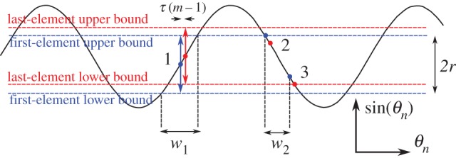
Illustration of frequency of occurrence (FoO) for m>1. The delay vector at location 1 is characterized by its first element (blue dot) and last element (red dot), and their bounds at ±r (blue and red dashed lines, respectively); the distance between the first and last elements, along the horizontal axis, is τ(m−1). For delay vectors from the positive slope, the similar ones are those which are inside the lower and upper bounds of the first element, the number of which is equivalent to w₁ on the horizontal axis. For delay vectors from the negative slope, the similar ones are those for which the first elements are less than the first-element upper bound, and for which last elements are greater than the last-element lower bound, the number of which is equivalent to w₂ on the horizontal axis.

Combining equations (A 3) and (A 4), an analytical solution for SE can be obtained by calculating the number of delay vectors similar to other delay vectors, for m and (m+1), and obtaining the average FoO values in the range θ_n∈[0,π/2] as

$$\begin{array}{r}\text{SE}=-\ln \left[\frac{(1/2\pi )(1/N_{\theta })\sum _{{\theta }_n=0}^{\pi /2}\{w_1({\theta }_n,r)+w_2({\theta }_n,r,m+1,\tau )\}}{(1/2\pi )(1/N_{\theta })\sum _{{\theta }_n=0}^{\pi /2}\{w_1({\theta }_n,r)+w_2({\theta }_n,r,m,\tau )\}}\right],\end{array}$$ A 5

where N_θ is the number of values of θ_n used for evaluation. Note that under the considered assumptions, $\tau <\arcsin (r)$, the range θ_n∈[0,π/2] is sufficient to evaluate SE as the FoO values will repeat for θ_n outside this range.

The above analysis allows us to examine the operation of SE for different frequencies. In the discrete case where the sampling frequency remains fixed, the same value of τ, and therefore also τ(m−1), will span increasing horizontal-axis distances for increasing sinusoid frequencies (figure 21). From equation (A 5), only w₂ will change for different frequencies. It is clear from equation (A 4) that, as τ(m−1) increases, w₂ will decrease. Note also that, as the ratio τ((m+1)−1)/τ((m)−1) will increase for increasing τ, the relevant ratio in equation (A 5), (a+w₂(θ_n,r,m+1,τ))/(a+w₂(θ_n,r,m,τ)), where a is a constant, will decrease for increasing frequency, ∀ θ_n∈[0,π/2]. Thus, as the negative logarithm of a decreasing value will increase (equation (A 5)), SE will increase for increasing frequency. The accuracy of the model in equation (A 5) is verified in figure 22 where, for increasing normalized frequency (the sampling frequency was 10 000 Hz), the SE calculated for the time series and the numerical evaluation of the model are observed to be similar. Observe that the model saturates for normalized frequencies exceeding 0.01 as one of the core model assumptions, τ(m−1) is small, is no longer valid. Note also that the empirically obtained SE simulation results also saturate. The model does not accommodate for scenarios where the frequency approaches the Nyquist frequency, where the number of similar delay vectors will be equal for m and m+1, and the SE is zero.

Figure 22.

SE analysis of discrete-sampled sinusoids of different frequencies. The solid black line shows the SE (m=2), for sine waves of normalized frequencies in the range [0.0001,0.1] for r=0.1 and r=0.2. The dashed red line shows the model-based SE estimate, described by equation (A 5), which matches the simulation results for sinusoidal data.

The model allows us to also examine the operation of SE for different sinusoid amplitudes. Increasing the sinusoid amplitude is equivalent to decreasing the distance threshold r. From figure 22, it is clear that the model supports the observation that SE decreases for increasing r. Thus, for increasing amplitude the SE will increase. This is in agreement with the reported operation of SE (both simulated and model-based) for the amplitude changes brought about in WGN caused by coarse-graining [31].

Ethics statement

All physiological recordings described in the manuscript were made with the gtec g.USBamp, a certified and FDA-listed medical device. Ethics approval was obtained from the Joint Research Office at Imperial College London, reference ICREC_12_1_1. Written consent was obtained for all volunteer subjects; the subjects were not paid for their participation.

References

- 1.Elbert T, Ray WJ, Kowalik ZJ, Skinner JE, Graf KE, Birbaumer N. 1994. Chaos and physiology: deterministic chaos in excitable cell assemblies. Physiol. Rev. 4, 1–47. [DOI] [PubMed] [Google Scholar]
- 2.Sweeney-Reed CM, Nasuto SJ. 2007. A novel approach to the detection of synchronisation in EEG based on empirical mode decomposition. J. Comput. Neurosci. 23, 79–111 (doi:10.1007/s10827-007-0020-3) [DOI] [PubMed] [Google Scholar]
- 3.Huang NE, Shen Z, Long SR, Wu MC, Shih HH, Zheng Q, Yen N-C, Tung CC, Liu HH. 1998. The empirical mode decomposition and the Hilbert spectrum for nonlinear and non-stationary time series analysis. Proc. R. Soc. Lond. A 454, 903–995 (doi:10.1098/rspa.1998.0193) [Google Scholar]
- 4.Schwartz M, Bennet WR, Stein S. 1966. Communications systems and techniques New York, NY: McGraw-Hill. [Google Scholar]
- 5.Chen X, Zhang Y, Zhang M, Feng Y, Wu Z, Qiao F, Huang NE. 2013. Intercomparison between observed and simulated variability in global ocean heat content using empirical mode decomposition, part I: modulated annual cycle. Clim. Dyn. 41, 2797–2815 (doi:10.1007/s00382-012-1554-2) [Google Scholar]
- 6.Tang L, Yu L, Wang S, Li J, Wang S. 2012. A novel hybrid ensemble learning paradigm for nuclear energy consumption forecasting. Appl. Energy 93, 432–443 (doi:10.1016/j.apenergy.2011.12.030) [Google Scholar]
- 7.Wu Z, Huang NE. 2004. A study of the characteristics of white noise using the empirical mode decomposition method. Proc. R. Soc. Lond. A 460, 1597–1611 (doi:10.1098/rspa.2003.1221) [Google Scholar]
- 8.Flandrin P, Rilling G, Gonçalves P. 2004. Empirical mode decomposition as a filter bank. IEEE Signal Proc. Lett. 11, 112–114 (doi:10.1109/LSP.2003.821662) [Google Scholar]
- 9.Rilling G, Flandrin P. 2008. One or two frequencies?: The empirical mode decomposition answers. IEEE Trans. Signal Process. 56, 85–95 (doi:10.1109/TSP.2007.906771) [Google Scholar]
- 10.Tanaka T, Mandic DP. 2007. Complex empirical mode decomposition. IEEE Signal Proc. Lett. 14, 101–104 (doi:10.1109/LSP.2006.882107) [Google Scholar]
- 11.Bin Altaf MU, Gautama T, Tanaka T, Mandic DP. 2007. Rotation invariant complex empirical mode decomposition. In Proc. IEEE Int. Conf. on Acoustics, Speech and Signal Processing (ICASSP 2007), Honolulu, Hawaii, 15–20 April 2007, vol. 3, pp. 1009–1012 Piscataway, NJ: IEEE. [Google Scholar]
- 12.Rilling G, Flandrin P, Gonçalves P, Lilly JM. 2007. Bivariate empirical mode decomposition. IEEE Signal Proc. Lett. 14, 936–939 (doi:10.1109/LSP.2007.904710) [Google Scholar]
- 13.Rehman N, Mandic DP. 2010. Empirical mode decomposition for trivariate signals. IEEE Trans. Signal Process. 58, 1059–1068 (doi:10.1109/TSP.2009.2033730) [Google Scholar]
- 14.Rehman N, Mandic DP. 2010. Multi-variate empirical mode decomposition. Proc. R. Soc. A 466, 1291–1302. [Google Scholar]
- 15.Wu Z, Huang NE. 2004. Ensemble empirical mode decomposition: a noise-assisted data analysis method. Adv. Adapt. Data Anal. 1, 1–41 (doi:10.1142/S1793536909000047) [Google Scholar]
- 16.Rehman N, Mandic DP. 2011. Filter bank property of multi-variate empirical mode decomposition. IEEE Trans. Signal Process. 59, 2421–2426 (doi:10.1109/TSP.2011.2106779) [Google Scholar]
- 17.Novak V, Yang AC, Lepicovsky L, Goldberger AL, Lipsitz LA, Peng C-K. 2004. Multimodal pressure-flow method to assess dynamics of cerebral autoregulation in stroke and hypertension. Biomed. Eng. Online 3, 39 (doi:10.1186/1475-925X-3-39) [DOI] [PMC free article] [PubMed] [Google Scholar]
- 18.Li X, Li D, Liang Z, Voss LJ, Sleigh JW. 2008. Analysis of depth of anesthesia with Hilbert–Huang spectral entropy. Clin. Neurophysiol. 119, 2465–2475 (doi:10.1016/j.clinph.2008.08.006) [DOI] [PubMed] [Google Scholar]
- 19.Silchenko AN, Adamchic I, Pawelczyk N, Hauptmann C, Maarouf M, Sturm V, Tassa PA. 2010. Data-driven approach to the estimation of connectivity and time delays in the coupling of interacting neuronal subsystems. J. Neurosci. Meth. 191, 32–44 (doi:10.1016/j.jneumeth.2010.06.004) [DOI] [PubMed] [Google Scholar]
- 20.Chen X, Wu Z, Huang NE. 2010. The time-dependent intrinsic correlation based on the empirical mode decomposition. Adv. Adapt. Data Anal. 2, 233–265 (doi:10.1142/S1793536910000471) [Google Scholar]
- 21.Park C, Looney D, Kidmose P, Ungstrup M, Mandic DP. 2011. Time-frequency analysis of EEG asymmetry using bivariate empirical mode decomposition. IEEE Trans. Neural. Syst. Rehabil. Eng. 19, 366–373 (doi:10.1109/TNSRE.2011.2116805) [DOI] [PubMed] [Google Scholar]
- 22.Hu M, Liang H. 2012. Adaptive multi-scale entropy analysis of multi-variate neural data. IEEE Trans. Biomed. Eng. 59, 12–15 (doi:10.1109/TBME.2011.2162511) [DOI] [PubMed] [Google Scholar]
- 23.Hu M, Liang H. 2012. Noise-assisted instantaneous coherence analysis of brain connectivity. Comput. Intell. Neurosci. 2012, 1–12 (doi:10.1155/2012/275073) [DOI] [PMC free article] [PubMed] [Google Scholar]
- 24.Rodrigues J, Andrade A. 2013. Instantaneous Granger causality with the Hilbert–Huang transform. ISRN Signal Processing 2013, 1–9 (doi:10.1155/2013/374064) [Google Scholar]
- 25.Tass P, Rosenblum MG, Weule J, Kurths J, Pikovsky A, Volkmann J, Schnitzler A, Freund H-J. 1998. Detection of n:m phase locking from noisy data: application to magnetoencephalography. Phys. Rev. E 81, 3291–3294. [Google Scholar]
- 26.Valera F, Lachaux J-P, Rodriguez E, Martinerie J. 2001. The brainweb: phase synchronization and large-scale integration. Nat. Rev. Neurosci. 2, 229–239 (doi:10.1038/35067550) [DOI] [PubMed] [Google Scholar]
- 27.Looney D, Park C, Kidmose P, Ungstrup M, Mandic DP. 2009. Measuring phase synchrony using complex extensions of EMD. In Proc. 15th IEEE/SP Workshop on Statistical Signal Processing (SSP '09), Cardiff, UK, 31 August–3 September 2009, pp. 49–52 Piscataway, NJ: IEEE. [Google Scholar]
- 28.Mutlu AY, Aviyente S. 2011. Multi-variate empirical mode decomposition for quantifying multi-variate phase synchronization. EURASIP J. Adv. Sig. Pr. 2011, 1–13 (doi:10.1155/2011/615717) [Google Scholar]
- 29.Richman JS, Moorman JR. 2000. Physiological time-series analysis using approximate entropy and sample entropy. Am. J. Physiol. Heart Circ. Physiol. 278, H2039–H2049. [DOI] [PubMed] [Google Scholar]
- 30.Costa M, Goldberger AL, Peng C-K. 2002. Multi-scale entropy analysis of complex physiologic time series. Phys. Rev. E 89, 068102. [DOI] [PubMed] [Google Scholar]
- 31.Costa M, Goldberger AL, Peng C-K. 2005. Multi-scale entropy analysis of biological signals. Phys. Rev. E 71, 021906 (doi:10.1103/PhysRevE.71.021906) [DOI] [PubMed] [Google Scholar]
- 32.Tsai P-H, Lin C, Tsao J, Lin P-F, Wang P-C, Huang NE, Lo M-T. 2012. Empirical mode decomposition based detrended sample entropy in electroencephalography for Alzheimer's disease. J. Neurosci. Meth. 210, 230–237 (doi:10.1016/j.jneumeth.2012.07.002) [DOI] [PubMed] [Google Scholar]
- 33.Lin P-F, Lo M-T, Tsao J, Chang Y-C, Lin C, Ho Y-L. 2014. Correlations between the signal complexity of cerebral and cardiac electrical activity: a multi-scale entropy analysis. PLoS ONE 9, e87798 (doi:10.1371/journal.pone.0087798) [DOI] [PMC free article] [PubMed] [Google Scholar]
- 34.Ahmed MU, Rehman N, Looney D, Rutkowski TM, Kidmose P, Mandic DP. 2012. Multi-variate entropy analysis with data-driven scales. In Proc. IEEE Int. Conf. Acoust. Speech. Signal. Process., pp. 3901–3904. [Google Scholar]
- 35.Cohen L. 1995. Time-frequency analysis Englewood Cliffs, NJ: Prentice-Hall. [Google Scholar]
- 36.Rilling G, Flandrin P, Gonçalves P. 2003. On empirical mode decomposition and its algorithms. In Proc. 6th IEEE/EURASIP Workshop on Nonlinear Signal and Image Processing (NSIP '03), Grado, Italy, 8–11 June 2003 Piscataway, NJ: IEEE. [Google Scholar]
- 37.Junsheng C, Dejie Y, Yu Y. 2006. Research on the intrinsic mode function (IMF) criterion in EMD method. Mech. Syst. Signal Process. 20, 817–824 (doi:10.1016/j.ymssp.2005.09.011) [Google Scholar]
- 38.Looney D, Mandic DP. 2009. Multi-scale image fusion using complex extensions of EMD. IEEE Trans. Signal Process. 57, 1626–1630 (doi:10.1109/TSP.2008.2011836) [Google Scholar]
- 39.Rehman N, Park C, Huang NE, Mandic DP. 2013. EMD via MEMD: multi-variate noise-aided computation of standard EMD. Adv. Adapt. Data Anal. 5, 1350007 (doi:10.1142/S1793536913500076) [Google Scholar]
- 40.Pereda E, Quiroga RQ, Bhattacharya J. 2005. Nonlinear multi-variate analysis of neurophysiological signals. Prog. Neurobiol. 77, 1–37 (doi:10.1016/j.pneurobio.2005.10.003) [DOI] [PubMed] [Google Scholar]
- 41.Pincus SM. 1991. Approximate entropy as a measure of system complexity. Proc. Natl Acad. Sci. USA 88, 2297–2301 (doi:10.1073/pnas.88.6.2297) [DOI] [PMC free article] [PubMed] [Google Scholar]
- 42.Masi CM, Hawkley LC, Rickett EM, Cacioppo JT. 2007. Respiratory sinus arrhythmia and diseases of aging: obesity, diabetes mellitus, and hypertension. Biol. Psychol. 74, 212–223 (doi:10.1016/j.biopsycho.2006.07.006) [DOI] [PMC free article] [PubMed] [Google Scholar]
- 43.Barnett L, Seth AK. 2011. Behaviour of Granger causality under filtering: theoretical invariance and practical application. J. Neurosci. Meth. 201, 404–419 (doi:10.1016/j.jneumeth.2011.08.010) [DOI] [PubMed] [Google Scholar]