Technical aspects of dental CBCT: state of the art

Abstract

As CBCT is widely used in dental and maxillofacial imaging, it is important for users as well as referring practitioners to understand the basic concepts of this imaging modality. This review covers the technical aspects of each part of the CBCT imaging chain. First, an overview is given of the hardware of a CBCT device. The principles of cone beam image acquisition and image reconstruction are described. Optimization of imaging protocols in CBCT is briefly discussed. Finally, basic and advanced visualization methods are illustrated. Certain topics in these review are applicable to all types of radiographic imaging (e.g. the principle and properties of an X-ray tube), others are specific for dental CBCT imaging (e.g. advanced visualization techniques).

Introduction

Soon after the development of the first CT scanner, the concept of CBCT was introduced in radiology.¹ It was first applied for angiography before being gradually introduced for other applications.^2–4

Development of specialized CBCT scanners for use in dentistry started in the second half of the 1990s.^5,6 Soon thereafter, the use of CBCT for dental, maxillofacial and ear–nose–throat applications started booming. Currently, CBCT is a widely used tool for several dental applications, such as implant planning, endodontics, maxillofacial surgery and orthodontics.⁷ Its widespread use has resulted in several concerns regarding justification and optimization of CBCT exposures, training of CBCT users and quality assurance of CBCT scanners.⁸ Therefore, it is important to have a full understanding of the technical principles of dental CBCT imaging in order to reap the full benefit of this technique while minimizing radiation-related patient risk.

This review provides an overview of technical aspects of dental CBCT imaging. Every part of the imaging chain is covered: hardware, acquisition, reconstruction, image visualization and manipulation. Many aspects of this review are applicable to all types of CBCT imaging, while others are specific to dental CBCT scanners.

Imaging hardware

X-ray tube

Basic principle

X-rays are generated in a tube containing an electrical circuit with two oppositely charged electrodes (i.e. a cathode and anode) separated by a vacuum (Figure 1). The cathode is composed of a filament that gets heated when an electric current is applied, inducing the release of electrons through an effect known as thermionic emission. Because of the high voltage between the cathode and anode, these released electrons will be accelerated towards the anode, colliding with it at high speeds at a location called the focal spot. Ideally, this focal spot is point sized, but typical focal spots in CBCT are 0.5-mm wide; the size of the focal spot is one of the determinants of image sharpness as shown further below. The anode consists of a high-density material (e.g. tungsten), which will collide with the incoming electrons. The energy generated through this collision is mainly lost as heat, but a small part is converted into X-rays through an effect known as Bremsstrahlung (see the X-ray spectrum and tube parameters section). X-rays are emitted in all directions, but absorption within the anode and the tube housing results in a beam emerging from the tube perpendicular to the electron beam. The anode surface is slightly tilted in order to maximize the outgoing X-ray fluence through the exit window of the tube.

Figure 1.

Simplified schematic of an X-ray tube. A current heats the filament at the cathode, leading to the release of electrons (e−) through the thermionic effect. These electrons are accelerated towards the anode by means of a high potential difference (kV). Through collisions of electrons with the anode target, X-rays are produced. Only X-rays going in the required direction for imaging are able to exit the tube; other X-rays are blocked at the border of the tube (hashed arrows).

To limit the patients' exposed area to that required for data acquisition, the beam is collimated by blocking X-rays that are not passing through the scanned volume. This is carried out using a lead-alloy collimator that has an opening (usually rectangular) for X-rays to pass through. Most CBCT systems have multiple pre-defined field-of-view (FOV) sizes, so a collimator will have several pre-defined openings according to the FOV sizes. On the other hand, a few CBCT machines have freely adjustable collimation along the z direction, allowing for FOVs of any height.

The basic principle of the X-ray tube is the same for each radiographic modality using X-rays. Differences between tubes used for two-dimensional (2D) radiography and CT and CBCT scanning are mainly found in the size of the exit window (i.e. collimation), the range of exposure factors and the amount of beam filtration (see the X-ray spectrum and tube parameters section).

X-ray spectrum and tube parameters

A beam emitted from an X-ray tube is polyenergetic and consists of photons with energies varying along a continuous spectrum. An X-ray spectrum as seen in Figure 2 shows the relative number of photons emitted as a function of photon energy. Spectra from diagnostic X-ray tubes have a continuous shape with a few sharp characteristic peaks. To understand the underlying factors and importance of the X-ray spectrum, the production of X-rays through the collision of electrons with an anode needs to be looked at in more detail. This article will provide a short but comprehensive description, but more details can be found in works such as Bushberg et al.¹⁰

Figure 2.

Examples of X-ray spectra for three tube voltages. Filtration is 2.5 mm aluminium in all cases. Spectral curves were plotted using the data from Birch and Marshall.⁹

The majority of photons in an X-ray beam are a result of an effect called Bremsstrahlung, which can be translated as “braking radiation”. Bremsstrahlung occurs in the X-ray tube when electrons, which are released from the cathode and accelerated towards the anode, interact with the anode material that slows down the electron to some extent. Following the law of conservation of energy, the loss of the electron's kinetic energy is partly compensated by the release of X-ray photons. The Bremsstrahlung energy spectrum is continuous, ranging between 0 keV (no deceleration) and a maximum value (full deceleration). In the absence of filtration, the photon incidence decreases with increasing energy. The maximum energy is determined by the tube potential, that is, a voltage of 90 kV between the cathode and anode results in a maximum X-ray energy of 90 keV.

The Bremsstrahlung spectrum is attenuated by internal (inherent) and external (added) filtration. Before exiting the X-ray tube, X-ray photons will interact with the tube housing, during which mainly low-energy photons are absorbed. Additional filtration in the form of metallic sheets is added to ensure that the majority of low-energy photons do not leave the tube, as these photons have a high probability of being absorbed within the patient (i.e. they are contributing to the patient's radiation dose but not contributing to the radiographic image). CBCT typically uses aluminium or copper filtration with an aluminium-equivalent thickness between 2.5 and 10 mm. The X-ray spectrum changes with the filter thickness; the mean or effective energy increases as the filter thickness is increased as shown in Figure 3. In addition to a reduction in entrance exposure, highly filtered X-ray beams suffer less from beam hardening (see Image quality section).

Figure 3.

X-ray spectral change caused by aluminium filter thickness. These spectra were calculated from Birch and Marshall.⁹ Tube voltage is 90 kV.

The discrete peaks appearing in an X-ray spectrum are a result of characteristic X-rays, which occur when the interaction of the electron beam with an anode atom results in the ejection of an electron in an inner shell. The vacant position is filled by an electron from an outer shell, resulting in the release of photons with an energy corresponding to the difference in energy between the shells' energy states. Therefore, these photons have specific energy quanta, characteristic of the anode material.

Unlike the tube voltage, tube current (mA) and exposure time are in direct proportion to the amount of X-ray photons exiting the tube and, therefore, to the radiation dose. The mA and exposure time are often combined as a product (mAs), which is thus also linearly proportionate to the dose. Any change made to the mAs does not affect the maximum or mean energy of the X-ray beam.

Gantry

Most dental CBCT systems use a fixed C-arm (i.e. a set-up in which X-ray tube and detector are connected using a rotatable, C-shaped arm), which usually rotates in the horizontal plane, allowing for seated and/or standing patient positioning (Figure 4). To position the FOV according to the region of interest (ROI), limited translation of the C-arm is usually possible within this plane as well as up–down movement, especially for scanners with a small FOV. Some scanners use supine patient positioning with a C-arm or fixed gantry, in which the tube and detector are rotating in the vertical plane (Figure 4).

Figure 4.

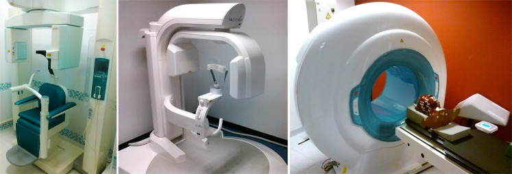
Different types of CBCT gantries. Left: seated patient position (3D Accuitomo^® 170; J. Morita, Kyoto, Japan). Middle: standing patient position (WhiteFox^®; Acteon Group, Mérignac, France). Right: supine patient position (NewTom^® 5G, QR srl, Verona, Italy).

Scanners allowing for standing patient positioning, which are usually accommodated for (wheel) chairs as well, occupy no more space than a panoramic radiography device. Scanners with a built-in chair or table occupy a larger space.

Source-to-object distances (SODs) and object-to-detector distances (ODDs) vary considerably between scanners. Together with the focal spot size, the SOD and ODD are important factors determining the sharpness of the projection images. The unsharpness at edges in the image caused by these geometric factors is referred to as “penumbra”, a Latin term that can be loosely translated as “almost shadow” (Figure 5). Larger SODs can lead to sharper images owing to reduction of focal spot blur, but shorter SOD gives a higher geometric magnification. There is therefore a trade-off between focal spot blur and geometric magnification that can be optimized relative to other factors such as FOV, X-ray scatter and entrance skin exposure. In addition, shorter ODDs (as well as larger SODs) allow for the use of smaller detector areas. On the other hand, shorter ODDs increase the proportion of scattered radiation reaching the detector. In practice, the ODD is typically as short as possible in order to reduce focal spot blur and increase the FOV.

Figure 5.

Effect of focal spot (FS) size, source-to-object distance (SOD) and object-to-detector distance (ODD) on penumbra (P). From top to bottom: a smaller focal spot, larger SOD and smaller ODD all decrease the penumbra width, which increases image sharpness.

Detector

X-ray detectors convert the incoming X-ray photons to an electrical signal and are therefore a crucial component of the imaging chain. The efficiency and speed at which the conversion is carried out are essential characteristics of X-ray detectors.

In dental CBCT imaging, different types of detectors are used. In early generation CBCT systems, image intensifiers were commonly used. Currently, different types of flat panel detectors (FPDs) are used instead, as these detectors are distortion free, have a higher dose efficiency, a wider dynamic range and can be produced with either a smaller or larger FOV. For a detailed description of image intensifiers vs FPD technology, see Baba et al¹¹ and Vano et al,¹² amongst others. Most existing CBCT systems use indirect FPDs where a layer of scintillator material, either gadolinium oxysulfide (Gd₂O₂S:Tb) or caesium iodide (CsI:Tl), is used to convert X-ray photons to light photons, which in turn are converted into electrical signals. Modern CsI scintillators have a higher image quality and dose efficiency because their columnar structure reduces the light spreading between the scintillators.

It is important to note that different components and technologies can be used for signal read-out in FPDs, and a distinction can be made between charge-coupled device (CCD), thin-film transistor (TFT) and complementary metal-oxide-semiconductor (CMOS) FPDs. These technologies differ in terms of detector size, pixel size, noise level, sensitivity and read-out speed and have varying cost efficiency depending on the total size of the detector (i.e. the need to add multiple, tiled panels in case of large detectors). CCDs are a mature technology offering high-speed read-out at high resolution, but they are limited to a fairly small FOV, and expanding the FOV using, for example, lens coupling or a fibre-optic taper, tends to reduce dose efficiency. FPDs based on active matrix TFT read-out arose in the late 1990s as a base technology for digital X-ray imaging and have also been incorporated in many applications of CBCT. More recently, CMOS detectors with a large FOV, fine resolution, high-speed read-out and low electronic noise are becoming available and incorporated within CBCT systems.

Image acquisition

Basic principles

During a CBCT scan, the X-ray tube and detector rotate along a circular trajectory (Figure 6). Typical rotation times range between 10 and 40 s, although faster and slower scan protocols exist. During the rotation, a cone- or pyramid-shaped X-ray beam results in several hundred 2D X-ray projections (i.e. raw data) being acquired by the detector (Figure 7). These projections can then be reconstructed into a three-dimensional (3D) representation of the scanned object (see the Image reconstruction section).

Figure 6.

To obtain projected images, the X-ray tube and detector move concomitantly around the rotation axis. 2D, two dimensional.

Figure 7.

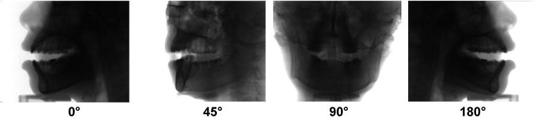
Two-dimensional projections at different angles. At a constant tube current, a higher overall detector signal is received for lateral views (0° and 180°) than for anterior/posterior views (90°).

Acquisition parameters

While the basic acquisition principle is the same for each CBCT device, important differences are apparent when comparing acquisition methods and parameters.

The first distinction that can be made is between pulsed and continuous exposure. Some X-ray tubes allow the exposure to be pulsed to ensure that there is no exposure being made between projections. Several CBCT devices use pulsed exposure, resulting in a large discrepancy between scan time (i.e. the time between the first and last projection) and exposure time (i.e. the cumulative time during which an exposure is made). For example, the total scan time may be 20 s, but each pulse may be just 10 ms (giving a total exposure time of 2 s for a scan with 200 projections). Other X-ray tubes allow only continuous exposure, for which the total scan time and exposure time are equivalent. The dose is proportional to the product of the exposure time and tube current (i.e., to the mAs; see X-ray spectrum and tube parameters section). Both pulse and continuous exposure approaches are susceptible to effects of detector lag, but pulsed X-ray systems may exhibit improved spatial resolution owing to reduced motion effect, that is, motion of the gantry during each exposure/read-out frame.

The second variable is the rotation arc. While most CBCT scanners acquire projections along a 360° angle (i.e. a full rotation of tube and detector), a rotation of 180° plus the beam angle (i.e. a half rotation) suffices for reconstruction of a full FOV. For some scanners, a partial rotation is used out of necessity, as a full rotation is not possible owing to mechanical obstruction of the C-arm. Other devices allow for the selection of a half or full rotation.

There are also potential dosimetric and image quality implications of a shorter scan arc. For some systems, the shorter scan entails a lower total mAs, so the effect of a partial rotation is similar to a reduction in mA or exposure time. In such cases, the reduction in radiation dose will be proportionate to the rotation arc, with 180° rotations resulting in a dose reduction of approximately 50%. However, the starting angle of the partial rotation has dosimetric consequences as well, owing to the asymmetrical distribution of radiosensitive organs in the head and neck. Several studies have shown the asymmetric dose distribution associated with scans for which the X-ray source traverses the posterior, lateral or anterior aspects of the head. The overall effect tends to be small.^13–16 Since several radiosensitive organs are found anterior in the head, a scan in which the source traverses the posterior has the obvious advantage (e.g. in dose to the eye lens) of self-attenuation by the skull and bulk volume of the head. For dental CBCT, however, since the FOV is typically anterior in the head, several radiosensitive organs (e.g. salivary glands) are posterior to the centre of the FOV, implying that they would receive a lower dose if the tube would move along the anterior side.

In terms of image quality, a partial rotation tends to decrease overall image quality, this is mainly apparent in the amount of noise associated with reduced mAs. Depending on the mA, a 180° rotation protocol can lead to a slight or more pronounced increase in noise than in a 360° protocol (Figure 8). Reduced sampling associated with a shorter scan can also result in a reduction in image quality for a shorter scan (even if the total scan mAs is the same), evident as a slight increase in view aliasing effects associated with a smaller number of projections. The view aliasing effects tend to be secondary to the quantum noise effects, and a full characterization of short scan vs 360° scans, as well as the effect (or lack thereof) of the starting angle on image quality has yet to be fully assessed.

Figure 8.

CBCT scan of a mandible at (a) 360° rotation, 70 mAs and (b) 180° rotation, 36 mAs showing little or no perceptible difference. Differences will be more pronounced at lower mA levels. Reproduced from Lennon et al¹⁷ with permission from John Wiley and Sons.

The dose associated with each scan is affected by a number of scan parameters selected by the user, either manually or through pre-set exposure protocols. For most CBCT systems, the kVp is fixed, and the tube current (mA) and exposure time (s) can be varied depending on the desired image quality and patient size. In current dental CBCT practice, this is typically performed either manually or through the selection of pre-set exposure protocols. Using automatic exposure control, which is commonly applied in medical CT, the exposure is varied before or during the scan automatically by a feedback circuit depending on patient size and attenuation, assuring no under- or overexposure takes place. Different types of automatic exposure control are being used in CT. One simple implementation in dental CBCT determines the mAs based on a 2D scout image. A lower detector signal for the scout image results in a higher mAs for the actual CBCT scan, and vice versa. This type of exposure control could be extended by adjusting the mA during the scan itself, varying the mA for each view. Depending on the position of the tube, the size and position of the FOV and the X-ray attenuation, the mA can be adjusted to keep the detector signal constant. This would lead to a lower mA in lateral views and a higher mA in posterior/anterior views (Figure 7). This can be performed in a pre-set method where the manufacturer has determined the relative mA needed at each angle. Ideally, the adjustment would be performed via real-time feedback to be truly considered as a patient-specific automatic exposure control method; at the time of writing this is not yet introduced in dental CBCT.

Image reconstruction

Pre-processing of raw data

Before reconstruction, the 2D projection data or raw data can undergo several pre-processing steps. These steps may vary between manufacturers and are typically performed to remove aberrations associated with variations in detector dark current, gain and pixel defects.

Common pre-processing tools are offset and gain corrections, which compensate for differences between detectors and between pixels of a detector in terms of sensitivity and correct for the “dark” signal (i.e. when no X-rays are used). In addition, an afterglow correction can be performed to remove the latent image of the previous projection, which is especially important when a large number of projections per second are acquired. Furthermore, blemishes due to faulty pixels or projection lines can be recognized and removed. Several other processing methods can be used; their efficiency is often dependent on the preciseness of the knowledge of the acquisition system (e.g. beam spectrum, scatter distribution, source-detector distance, detector response etc.).

Reconstruction algorithms

Image reconstruction is a technique to reconstruct an image from multiple projections. The reconstructed image represents the relative X-ray attenuation (i.e. the reduction of beam intensity owing to X-ray interactions) of the different materials in the object. In CBCT, the scanned object is reconstructed as a 3D matrix of voxels (often—but not necessarily—with isotropic voxel size in the x, y and z directions), with each voxel being assigned a grey value depending on the attenuation of the material(s) inside it (Figure 9). This stack can be shown in 3D or along different planes for visualization in 2D (see Image visualization section). Standard triplanar views include axial, sagittal and coronal slices as well as oblique slices through the reconstructed volume.

Figure 9.

Reconstructed axial CBCT images using filtered backprojection reconstruction.

In general, image reconstruction can be grouped into three categories: filtered back projection (FBP),^18,19 algebraic reconstruction techniques (ARTs)^18,20 and statistical methods.^21–24

The most widespread form of 3D FBP used in CBCT uses the Feldkamp–Davis–Kress (FDK) algorithm,¹⁹ which is used in almost all CBCT machines owing to its simplicity and fast reconstruction times. While projection data are a summation of linear attenuation coefficients along a ray path that can be called forward projection, FBP (and the FDK algorithm) is basically the inverse or back projection process of the weighted and filtered projections, in which the value for each pixel in the projection image is assigned to every voxel along the path of the X-ray (Figure 10). When this is performed for every projection, an image of the scanned object is reconstructed. The filter consists of two parts: (1) a ramp filter to correct for blur that is intrinsic to the projection/back projection process and (2) a smoothing filter to reduce high-frequency noise that is amplified by the ramp filter. Such smoothing filters are optional and adjustable according to their cut-off frequency, which can be expressed as a fraction of the Nyquist frequency (i.e. the highest displayable frequency in an image). Smoothing filters can significantly affect image quality by reducing noise at the cost of spatial resolution. Examples of reconstruction filters ranking from the sharpest to smoothest include Ram-Lak (a pure ramp filter), Shepp–Logan, Cosine, Hamming and Hann. The cut-off frequency of such filters is freely adjustable: the higher the cut-off frequency, the sharper but noisier the reconstructed image (Figure 11). Some software may allow a user to adjust reconstruction parameters as desired for a particular imaging task.

Figure 10.

Image reconstructed using filtered backprojection with a different number of projections. When a low number of projections is used, the object is undersampled, and images exhibit streaks along the direction of backprojected rays. An improved reconstruction is possible when the number of projection angles is increased.

Figure 11.

CBCT images showing the effect of different cut-off frequencies (expressed as a fraction of the Nyquist frequency) using cosine reconstruction filters. A larger cut-off frequency increases both spatial resolution and noise.

ARTs involve an iterative process in which the image reconstruction (i.e. the attenuation coefficient for each voxel) is successively estimated through repeated comparison of the projection data and the current image estimate. After an initial reconstruction is obtained (for example, by FBP), the image is adjusted according to what the projection data arising from the current reconstruction estimate would be. These are compared with the actual projection data, after which a new, corrected reconstruction is obtained. This process is repeated until a specified level of acceptability is reached—according to a “stopping criterion” determined by either diminishing change from one iteration to the next or a maximum number of iterations. Owing to this iterative process, ART requires much more computation time than FDK. Although ART can produce better image quality than FDK and allows for great versatility, neither of these reconstruction techniques takes noise explicitly into account, which is ubiquitous in real projection data.

Unlike ART, statistical image reconstruction is an iterative technique that reconstructs an image based on a statistical model of the projection data. Since noise is intrinsic to the incident and detected number of X-rays (e.g. according to a Poisson random distribution of X-ray quanta), it is reasonable to model the physics of data acquisition as Poisson noise, Gaussian noise or a combination of both. At each iteration, the measurement data are compared with the estimated measurement from the corresponding model. Examples of statistical image reconstruction include maximum-likelihood estimates expectation–maximization,²³ maximum-a-posterior,²⁵ penalized likelihood²¹ and ordered subset expectation–maximization.^26–28 Although statistical methods have proven benefits over FDK reconstruction, particularly under conditions of low dose (high noise) and/or a lower number of projections, they are not commonly implemented in dental CBCT systems owing to a large computation time.

Image stitching

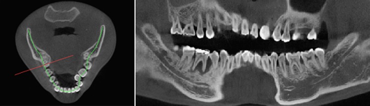
In some cases, multiple consecutive scans are acquired, which are then merged (i.e. stitched) into one image. This can be carried out to combine two or more small-diameter FOVs or two small-height FOVs (Figure 12). Between the scans, the chair or C-arm moves along a pre-set distance, leaving a small overlap between the images. Stitching of the image could be carried out through simple overlap (as the relative movement of the patient between scans is known exactly) or through automatic matching of the images using image registration.²⁹

Figure 12.

Image stitching in CBCT. Left: large-diameter field of view (FOV) covering the entire mandible. Right: stitching of three small-diameter FOVs, covering the dentition of the mandible.

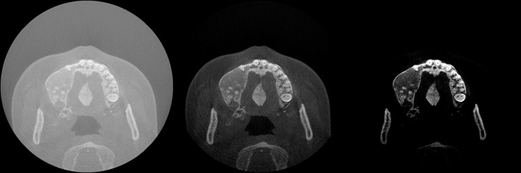
Grey value calibration

A reconstructed image in CT or CBCT has a grey value assigned to each voxel. In general, grey values are generic, whole numbers, with lower numbers corresponding with darker voxels (Figure 13). How light or dark a voxel will appear on the screen depends on the visualization software (see the Image visualization section). The amount of possible grey values for a given image (i.e. the grey value range) depends on the bit depth of the image, with an image of n bit having 2ⁿ possible grey values (e.g. 12 bit = 2¹² = 4096 grey values).

Figure 13.

Grey values (left) and displayed image (right) of a 10 × 10 pixel image. Although the image in question is 8 bit (i.e. 256 possible grey values), only 3 grey values are used in this case.

In CT imaging, grey values can be calibrated as Hounsfield units (HU), which express the relative X-ray absorption of a voxel in relation with the absorption of air and water:

$$\text{HU}=1000\hspace{0.17em}\times \hspace{0.17em}\frac{{\mu }_{\text{voxel}}-\hspace{0.17em}{\mu }_{\text{water}}}{{\mu }_{\text{water}}}$$

with μ_voxel and μ_water being the linear attenuation coefficients for the voxel and water, respectively. According to this scale, the HU of water is 0, the HU of air is −1000 (μ_air = 0) and materials that absorb more X-rays have a higher HU value. HU can serve various purposes, such as the classification of trabecular bone for implant placement and the differential diagnosis of lesions.

The applicability of HU in CBCT is hampered owing to several reasons, such as excessive scattered radiation and errors from data truncation (i.e. mass outside the FOV influencing grey values inside it). The resulting uncertainty related to HU accuracy and consistency is often too large for routine clinical application.³⁰ Even for CBCT images in which grey values are distributed along a pseudo-HU scale (i.e. with a minimum value of −1000), the quantitative use of grey values should be avoided in current dental CBCT systems. More information on this topic is given in the specific review on this topic, which can be found in this issue.³¹

Geometric calibration

Accurate image reconstruction requires calibration of the imaging system geometry.³² A geometric calibration, typically performed using manufacturer-specific test objects containing high-contrast markers or objects with known distances and shapes, defines the position of the X-ray source and detector for each projection view. Errors in geometric calibration may be evident as streaks and/or distortion in image reconstructions. FPDs are essentially distortionless, whereas X-ray image intensifiers often require an additional distortion correction to account for pincushion effects as illustrated in Figure 14. For each projection in the scan orbit, the geometric calibration characterizes the pose of both the X-ray source and detector, which is essential for accurate back projection in the reconstruction process. It is not essential that the X-ray source and detector follow a perfect circular orbit in the scan, but the orbit must be reproducible and accurately described by the calibration to avoid artefacts. Example artefacts associated with geometric calibration errors are shown in Figure 15, which illustrates CBCT images of a head phantom in the region of the temporal bone with various forms of possible geometric calibration errors. The images were acquired from a full 360° rotation and, as in Figure 15a,b, exhibit good visualization of bony details. A geometric calibration artefact associated with a systematic shift in the position of the centre of rotation or position of the piercing ray is shown in Figure 15c, creating a double image for the 360° acquisition (and a crescent-moon artefact for shorter scan orbits). The result of random errors in geometric calibration, for example, a poor estimate of high-frequency vibration/jitter in the system geometry, is shown in Figure 15d, creating streaks that can be difficult to distinguish from other sources of noise and streak artefacts. Daly et al³³ showed the type of artefact associated with various types of calibration errors and the sensitivity to each degree of freedom in a CBCT scanner.

Figure 14.

CBCT image of test object (SEDENTEXCT QI; Leeds Test Objects, Boroughbridge, UK) for analysis of geometric distortion, using 2-mm diameter, 3-mm deep recesses in a grid pattern with 10-mm spacing between adjacent recesses.

Figure 15.

Illustration of artefacts arising from geometric calibration errors. (a, b) Images of head phantom with accurate geometric calibration. (c) The same image as (b) reconstructed with a systematic error in calibration (viz., a five-pixel shift in the position of the piercing ray). (d) The same image as (b) reconstructed with a random error in calibration (viz., a four-pixel standard deviation about the true position of the piercing ray).

Image quality

The basic image quality characteristics of a medical image can be described using four fundamental parameters: spatial resolution, contrast, noise and artefacts. The exact definition of these parameters and the way they are estimated or quantified for a medical image may differ. In addition, some of these parameters are inter-dependent, for example, the classic interdependence and trade-off between spatial resolution and noise, implying that all four parameters should always be considered together when judging the quality of image. Moreover, the quality of an image should be assessed relative to the imaging task, for example, detection of bone fracture or visualization of a soft-tissue abnormality, and the objective assessment of imaging performance should be understood relative to the task.

Spatial resolution, or sharpness, refers to the ability to discriminate small structures in an image. In CBCT imaging, spatial resolution is determined by many factors, such as focal spot size, detector element size, smoothing filter and reconstructed voxel size. Although CBCT is in general considered to have a high spatial resolution compared with multidetector CT, stemming from the use of smaller detector elements and thus, smaller voxel sizes, large differences have been reported between and within models.³⁴ The spatial resolution of the imaging system can be characterized in terms of the modulation transfer function (MTF), which describes the ability of the system to transfer signal of a given spatial frequency. Systems with higher spatial resolution have higher MTF, for example, they are better able to transfer high-frequency image information. For further information on spatial resolution, please refer to the dedicated article on spatial resolution in this issue.³⁵

The contrast of a radiographic image is defined by the ability to distinguish tissues or materials of different densities. It too depends on many factors, such as the dynamic range (i.e. the detectable range of exposure values) of the detector, the exposure factors and the bit depth of the reconstructed image. In addition, the perceived contrast depends on display settings such as window/level (see the Image visualization section). In its most basic form, contrast refers simply to the difference in mean voxel value between two regions of an image, for example, the mean difference in voxel value between a region of fat and a region of adjacent muscle. Contrast is a “large area” characteristic of the imaging system and is appropriate in description of large, slowly varying characteristics of the image. For small features, description of image quality in terms of contrast alone is limited, since the ability to resolve details is closely tied to the MTF. Again, more information on MTF can be found in the above-mentioned article on spatial resolution in this issue.³⁵

Noise refers to the random variability in voxel values in an image. There are different sources of noise in radiographic images, mainly:

• quantum noise: caused by the inherent random nature of the interactions happening during X-ray production and attenuation

• electronic noise: caused by the conversion and transmission of the detector signal.

Noise and spatial resolution are often managed in a trade-off, since many factors that improve one (e.g. voxel size, reconstruction filter etc.) degrades the other. Noise in CBCT is often higher than in conventional diagnostic CT owing to a relatively high amount of electronic noise in the detector and other factors.

Taken together, the contrast and noise (or contrast-to-noise ratio) is a simple metric of imaging performance with respect to large structures of varying attenuation (e.g. discrimination of bony lesions).

Image artefacts can be defined as regions in the image that are aberrant, that is, do not correspond to the real object, and are deterministic (i.e. non-random) with respect to the projection data. Various types and sources of artefacts exist in CBCT. Among the major sources of artefacts in CBCT is X-ray scatter, which can result in shading and streaks similar in appearance to beam-hardening effects (described below). X-ray scatter artefacts arise from data inconsistencies associated with X-ray photons undergoing Compton interactions in the patient (compare photoelectric absorption) and reaching the detector. Such false increases in signal results in an underestimate of attenuation values, for example, a darkening of the image reconstruction. Antiscatter grids can be employed to reduce X-ray scatter reaching the detector, but may carry an increase in dose. Scatter correction algorithms also exist in many forms, including simple parametric estimates of the (constant or low-order polynomial) background signal and more sophisticated Monte Carlo estimation of the scatter contribution in each projection.

Other common artefacts in dental CBCT are metal artefacts, which are the result of high X-ray absorption by high-density objects. Various effects contribute to metal artefacts, and the manner in that they appear in the image depends on the severity of these effects and the way the reconstruction algorithm deals with them.³⁶ One particular contributing effect (which also occurs without the presence of metal) is beam hardening. As seen in the X-ray spectrum and tube parameters section, an X-ray beam consists of a spectrum of energies with a maximum energy determined by the kVp and a mean energy at about 60% of the maximum. When passing through a given material, low-energy X-rays have a greater probability of being absorbed, and the mean energy of the beam increases (i.e. the same effect as in filtration). This increase of energy is what is called “hardening”. Basic reconstruction algorithms commonly assume a mono-energetic beam; therefore, regions adjacent to, or surrounded by, structures that cause beam hardening are falsely considered as radiolucent because the beam passed through them with relative little absorption. Thus, these regions will appear darker. Beam hardening can occur at any beam energy and for any material and tends to be more pronounced for low-energy beams and for denser materials (Figure 16). Beam hardening can be (partially) corrected during calibration and/or through the use of advanced iterative reconstruction algorithms, which, during each iteration, estimate the extent of beam hardening and correct for it.

Figure 16.

Beam hardening in CBCT. Top: axial slice of a small-sized phantom containing an aluminium cylinder. Bottom: plot profiles showing the variation of grey values along the diameter of the cylinder owing to beam hardening. A higher kVp reduces beam hardening; a change in mAs affects noise but not beam hardening.

It is important to note that a CBCT user has little influence on metal artefacts, as increasing exposure settings (e.g. mA and number of projections) do not improve the appearance of metal artefacts substantially enough to justify the increased radiation dose.³⁷ Metal artefacts can be reduced during reconstruction through the application of various types of metal artefact reduction techniques.³⁸ Metal artefact reduction technology in dental CBCT is currently being applied by certain manufacturers but is still somewhat underdeveloped and should be used with caution.

Other types of artefacts exist in dental CBCT. Because the diameter of the FOV usually does not cover the entire patient's head, truncation artefacts may occur. Another source of artefacts is patient motion. Depending on the amount of motion during image acquisition, slight blurring or severe artefacts may occur. Due to the relatively long scan times in CBCT, motion is an important issue. For patients at risk for excessive motion, a protocol with a short scan time can be selected.

Optimization of exposure in CBCT

Optimization of protection, as defined by the International Commission on Radiological Protection (ICRP), entails that the “likelihood of incurring exposure, the number of people exposed, and the magnitude of their individual doses should all be kept as low as reasonably achievable, taking into account economic and societal factors”.³⁹ It is a fundamental principle with a wide array of interpretations. In this section, a basic overview will be given of the effect of different imaging parameters on image quality and radiation dose, and how this relates to optimization.

Table 1 shows the relation between imaging parameters (i.e. kV, mAs, FOV size and voxel size) and image quality parameters (spatial resolution, contrast, noise and artefacts) as well as radiation dose. In terms of optimization, the most straightforward imaging parameter is FOV size, as larger FOVs increase radiation dose to the patient. In addition, larger FOVs increase the relative amount of scattered radiation reaching the detector, leading to an increase in noise and artefacts. On the other hand, small-diameter FOVs increase the “local tomography” or truncation effect due to the presence of asymmetrical mass outside the FOV affecting the projection data (i.e. for those beam angles that pass through the mass in question). As reconstruction algorithms cannot fully compensate for this effect, it can lead to various image aberrations such as shading (i.e. a gradient of darkening towards one side of the image) and truncation artefacts. However, the local tomography effect mainly affects the quantitative use of grey values, which is often not a critical component of CBCT performance anyway. Therefore, FOVs should always be kept as small as possible, covering only the ROI.

Table 1.

Effect of imaging parameters on image quality and radiation dose

Imaging parameter	Spatial resolution	Contrast	Noise	Artefacts	Radiation dose
FOV size ↑a	–	↓	↑	↑	↑
kV ↑	–	↓	↓	–b	↑
mAs ↑	–	–	↓	–	↑
Voxel size ↑	↓	–	↓	–	–

↓, decrease; ↑, increase; FOV, field of view; kV, tube voltage; mAs, tube current-exposure time product.

^aMinor image quality effects due to factors like beam divergence and truncation of the FOV not being taken into account.

^bBeam hardening is somewhat reduced at higher tube potential values (Figure 16).

Although kV and mAs have a similar overall effect, there is an important difference between them. Both factors, when increased, will primarily increase radiation dose and decrease noise owing to the increase of the total amount of emitted X-rays. Accordingly, the contrast-to-noise ratio will increase. In terms of optimization, the kV and mAs levels should be selected according to the required image quality and patient size, ensuring that image quality is adequate for a particular imaging task at the lowest possible dose. However, the effect of kV is more intricate, as it also affects the detection efficiency of the detector and the relative contribution of X-ray scatter, among others. Seeing that the amount and nature of X-ray interactions (absorption and scatter) varies with X-ray energy, both contrast and dose are affected. At fixed dose levels, the optimal kV settings in dental CBCT depends on the imaging task (e.g., visualization of high-contrast details or low-contrast soft tissues), although recent research on a certain CBCT model indicated that, considering a range of 60–90 kV, an increased kV results in a higher contrast-to-noise ratio at identical dose levels.⁴⁰

Strictly speaking, changing the voxel size does not affect radiation dose, as this is a freely adjustable reconstruction parameter. Larger voxel sizes decrease noise at the cost of image sharpness and vice versa. In practice, some manufacturers implement pre-set “resolution” protocols, for which smaller voxel sizes correspond with higher mAs values in order to keep noise relatively constant.

Image visualization

Multiplanar reformatting

A cone beam reconstruction process creates a 3D matrix that can be viewed as a series of 2D cross-sectional images—axial, sagittal and coronal views. Axial planes are a series of slices from top to bottom in the volume. Sagittal planes are a series of 2D slices from left to right, and coronal planes are a series of 2D slices from anterior to posterior. In a multiplanar reformation (MPR) window, these three orthogonal planar views are related through intersection lines or crosshairs, allowing for straightforward orientation and navigation (Figure 17).

Figure 17.

Multiplanar reformation. A, C and S indicate intersection lines corresponding with axial, coronal and sagittal planes, respectively.

Oblique and curved reformatting

Once volumetric images are created, besides multiplanar reformation, oblique reformation allows the user to cut through the FOV at any angle (Figure 18). The manipulation for oblique reformation can be performed either by rotating the image itself or rotating the intersection lines (as well as drawing new lines) as shown in Figure 19. Since voxels in oblique planes are not aligned either horizontally or vertically, oblique reformation requires interpolation.

Figure 18.

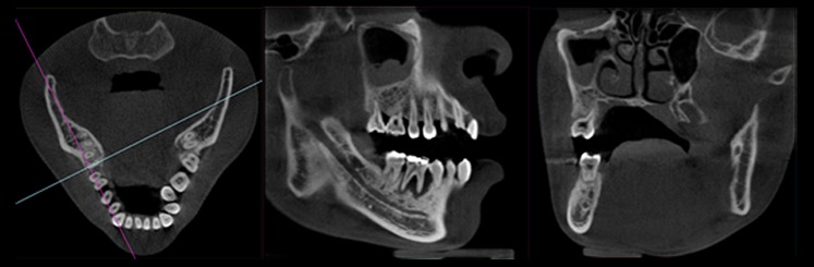
Oblique reformation. Lines in the axial plane (left) indicate the rotated sagittal (middle) and coronal (right) planes.

Figure 19.

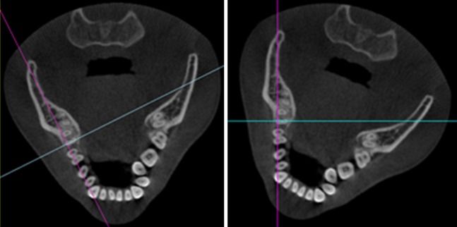
Manipulating oblique reformation by rotating intersection lines (left) or rotating the image itself (right).

Furthermore, reformation can be performed along a manually or automatically drawn curve. Most commonly, a panoramic curve is drawn along the dental arch to generate a series of synthetic panoramic views of the teeth and bone (Figures 20 and 21). Because of the small thickness of these synthetic panoramic images, it is often not possible to visualize the upper and lower dental arch in one image. Therefore, it is usually needed to draw separate curves for the upper and lower dental arches (Figure 22). Alternatively, a ray sum of these synthetic panoramic views can be calculated that resembles an image acquired from a panoramic radiograph. Figure 23 shows a ray sum panoramic image at different thicknesses of synthetic panoramic stacks.

Figure 20.

Synthetic panoramic images (right) along a curve drawn by the user in the axial plane (left).

Figure 21.

Additional synthetic panoramic images along curves slightly anterior or posterior to the one shown in Figure 20.

Figure 22.

Synthetic panoramic images for upper (top) and lower (bottom) jaw.

Figure 23.

Synthetic ray sum images at different thicknesses.

In addition to synthetic panoramic images, cross-sectional images can be derived from lines perpendicular to the panoramic curve (Figure 24).

Figure 24.

Left: position of cross-sectional images, perpendicular to the panoramic curve, displayed on an axial slice. Right: cross-sectional images at various positions along the curve.

Other visualizations

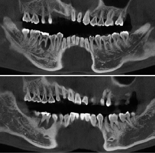
Apart from displaying a series of 2D images at particular planes, 3D renderings can be created. A distinction can be made between surface and volume rendering. Surface rendering (also known as indirect volume rendering) is a technique to transform the image data into geometric primitives and render them; some loss of information may therefore occur. One classification of surface rendering techniques is isosurfacing, such as the marching cubes algorithm,⁴¹ which produces surfaces having the same isosurface value, that is, it displays only the surface of thresholded areas (Figure 25). For simplicity, some viewer software has set pre-defined threshold values for different anatomical structures. From Figure 25, different threshold values result in different forms of 3D surface rendering, thus one needs to keep in mind that 3D rendering is for visualization purposes only, not for diagnosis and analysis. A variety of 3D image qualities with varying render times can be provided by the visualization software.

Figure 25.

Surface rendering with different threshold adjustment. A “threshold from x to y” implies that only grey values between x and y are retained for visualization. Grey values on this CBCT scan are not Hounsfield units.

Unlike surface rendering, volume rendering (also known as direct volume rendering) is a visualization technique that renders every voxel in the 3D volume data directly without intermediate geometry conversion, hence it produces a higher quality of visualization than does surface rendering. A popular volume rendering technique is ray casting,⁴² where each ray is cast from the view point to the volume data. Along the ray path, the sampling points are computed using interpolation and then their corresponding colours and opacities are composited into a final pixel colour on the 2D viewing plane. The colour and opacity transfer functions can be modelled to distinct different materials. Figures 26 and 27 show examples of volume-rendering displays with different transfer functions.

Figure 26.

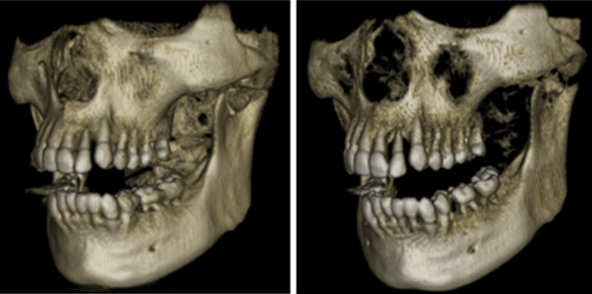
Volume rendering using different oblique transfer functions with varying threshold values.

Figure 27.

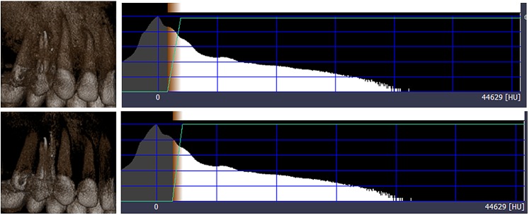
Volume rendering using transfer function adjustment with varying threshold values.

Maximum intensity projection is a special case of volume rendering. As the name implies, maximum intensity projection displays the maximum intensity or the brightest pixel value at each line originating from the viewpoint that passes through the object (Figure 28).

Figure 28.

Maximum intensity projection volume rendering.

Although the quality of 3D surface rendering is inferior to that of volume rendering, surface rendering is very useful when one wants to generate a drilling or surgical guide for implant placement by using a rapid prototyping machine or to print out the real physical model of the rendered object for treatment planning. To do this, the 3D object can be exported in a stereolithography file format. This benefit is unavailable for volume rendering since it provides only a 2D viewpoint; therefore, it cannot be exported as a 3D object for the preparation of guided surgery. However, some proprietary software might directly generate the final 3D model or a surgical guide without the need of exporting a stereolithography file as an intermediary step.

Image manipulation

After reconstruction, CBCT images can be manipulated in different ways to optimize the visualization of anatomical structures and lesions and to isolate (i.e. segment) certain parts of the image.

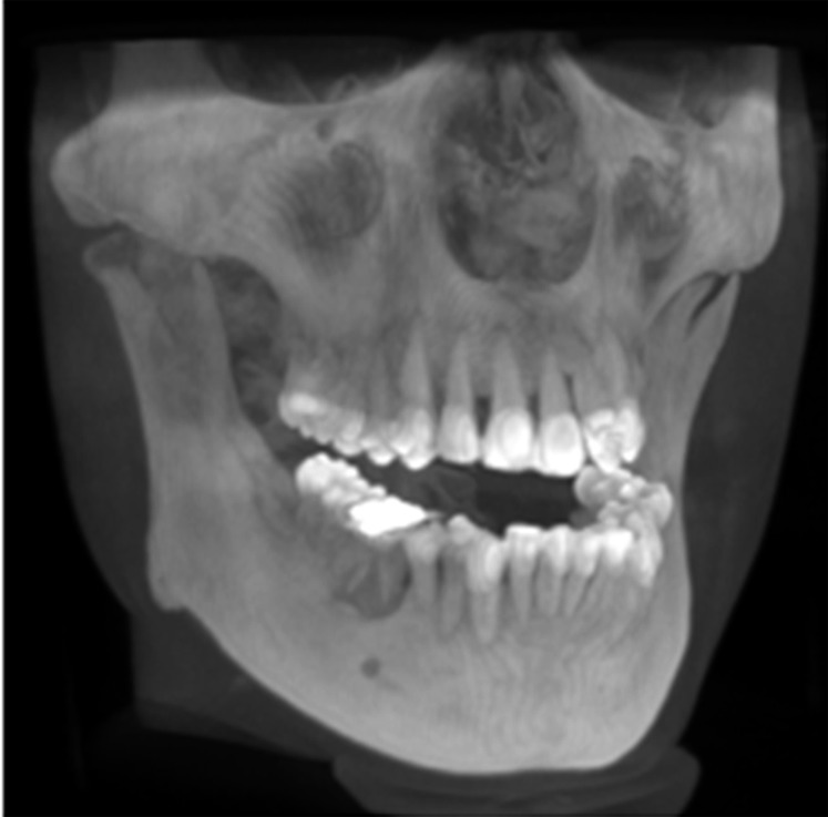
The most basic manipulation is the window/level transformation. This transformation is performed to optimize contrast in the image, by displaying only part of the full grey value range. This amount is determined by the window width (W). For example, a W of 1000 implies that 1000 grey values are considered for display, with the lowest grey value (and all values below it) being displayed as black and the highest (and all above it) as white. The window level (L) determines the central grey value within the window width. For example, a W/L of 1000/0 implies that grey values between −500 and +500 are considered for display, with all other values showing as black (<−500) or white (>+500). That way, the full contrast of the display monitor, and the human eye, is applied to this particular grey value range. W/L operations can be used for different purposes; in dental CBCT, it is mainly used to optimize contrast in the bone density range, that is, by using L-values corresponding to bone grey values (Figure 29).

Figure 29.

The effect of window/level. Left: large-width window covering the entire grey value range of the image, leading to poor image contrast. Middle: medium-width window covering soft-tissue and bone grey values, leading to good overall contrast. Right: small-width window with a high-level value, leading to high contrast for bone and teeth.

Basic filtering can also be applied, both during and after reconstruction, in order to smooth or sharpen the image. Alternatively, the image can be smoothened by increasing the slice thickness (Figure 30). By averaging multiple consecutive slices, image noise can be reduced at the cost of image sharpness (Figure 31). It can be recommended that the slice thickness should not be increased considerably when the visualization of small details is needed. Slice thickness should not be confused with slice interval (Figure 32), which changes the number of slices but does not alter image quality within a slice. The slice interval is often increased before exporting CBCT images in order to limit the size of the data. It should be performed with some care owing to the loss of information between slices, although this can be partly compensated by exporting coronal and sagittal stacks in addition to axial images. Slice thickness and slice interval are often selected concomitantly; it is important that the user understands the relevance of these parameters and chooses appropriate values according to the diagnostic task. For example, it can be recommended that—during initial radiological evaluation—both slice thickness and slice interval values should be as small as possible (e.g., identical to the voxel size) when the visualization of small details is needed.

Figure 30.

Increasing the slice thickness implies that a new image (e.g. Slice 1*) is created, in which each slice is the average of multiple (in this case, two) slices of the original image. The total number of slices does not change.

Figure 31.

Increasing the slice thickness reduces both sharpness and noise. Voxel size of the image is 0.25 mm. All images are zoomed to 800% for the purpose of illustration.

Figure 32.

Increasing the slice interval (SI) implies that a fraction of the slices (in this case, 50%) is discarded. The fraction of slices that remains is equal to the voxel size divided by the SI (e.g. 0.25-mm voxel size, 0.5-mm slice interval: 50% of slices remain). The total number of slices decreases with increasing SI, but the image quality within each slice does not change (e.g. Slice 1 is identical to Slice 1*).

Performing a zoom reconstruction is another option to highlight details in part of the image. The principle of zoom reconstruction was introduced by a few manufacturers after it became that large-FOV CBCT scans could not be reconstructed at small voxel sizes owing to the excessive increase in file size and reconstruction time. Owing to these technological limitations, large-FOV scans could not be displayed at their inherent sharpness, with the voxel size serving as a bottleneck.³⁴ To cope with this, the user can select a small ROI in the image and reconstruct that ROI at a smaller voxel size (Figure 33), increasing sharpness at the cost of higher noise. This zoom reconstruction is performed using the original raw data, avoiding the need for additional patient exposure when a high-resolution view is needed in addition to the large-FOV scan.

Figure 33.

Zoom reconstruction. (a) Large field-of-view scan showing region of interest of 4 × 4 × 4 cm (circles). (b) The original scan had a voxel size of 0.25 mm. (c) The zoom reconstruction had a voxel size of 0.08 mm.

In order to visualize or quantify a certain structure, the image can also be segmented, which is the division of an image in distinct regions (i.e. segments). Segmentation is widely used in all forms of medical imaging, and a plethora of techniques are available to accurately delineate the ROI. Although manual segmentation can be used in some cases, it is prone to error and can be time consuming when delineating a large volume slice by slice. A common segmentation technique is thresholding, in which the image is divided according to the grey values. All voxels with grey values above a certain limit (i.e. threshold) are grouped together, and all voxels with a grey value below the threshold are grouped. It is also possible to use double or multiple threshold values. The most common application of thresholding in dental CBCT is to discriminate bone from other tissues (e.g. in 3D rendering, as described above). It can also be used to measure the volume of the airways or sinus.⁴³ It should be noted that, owing to the absence of quantitative grey values in CBCT (see Grey value calibration section), thresholding is often performed manually. Adaptive thresholding techniques (i.e. automatic threshold determination based on the distribution of grey values in the image histogram) and other automatic thresholding criteria have been developed but are not yet widely used in dental CBCT.⁴⁴ Established advanced segmentation methods, based on edge detection, region growing or other techniques are largely absent in clinical CBCT imaging.

Display

Because of the use of window/level and zooming tools in digital imaging, display monitor requirements for CBCT images are relatively low. The main criteria are related to the size and resolution of the monitor, as images should be displayed at their native resolution (i.e. a 1:1 ratio between the display pixel and the image pixel) or better (i.e. having multiple display pixels for every image pixel) for optimal image sharpness. Contrast ratio and luminance should also be at an acceptable level, but are of secondary importance compared with the monitor resolution. Similarly, monitor settings such as contrast and gamma are not essential and will not be covered in this review.

To illustrate the importance of monitor size and resolution, imagine a 60 × 60-mm CBCT image with a voxel size of 0.1 mm. Every slice in this image will be 600 × 600 pixels. When visualizing this image using a multiplanar reformatting, a monitor will require a minimum resolution of 1200 × 1200 pixels to show each slice at a 1:1 ratio. In practice, owing to the graphic user interface of the viewing software occupying part of the screen, a monitor with a height of 1200 pixels would not suffice in this case. Therefore, the use of large-size, high-resolution monitors can be advocated, and users should make full use of zooming tools and maximize windows whenever applicable in order to ensure that the display monitor does not serve as a bottleneck for image sharpness (Figure 34).

Figure 34.

Display of a 170 × 170 × 120-mm CBCT scan with a 0.25-mm voxel size (680 × 680 × 480 voxels) on a 21.5-inch monitor with a resolution of 1920 × 1080 pixels. In multiplanar reformation mode (left), approximately 0.4 monitor pixels are used for each image pixel, making the monitor a limiting factor for image sharpness. When maximizing the axial slice (bottom), approximately 1.8 monitor pixels are used for each image pixel. The graphic user interface of the software and part of the viewer window was cropped from the image. Left and right images are to scale.

Conclusions and future prospects

This review described the basic concepts of CBCT imaging, covering each part of the imaging chain. Although it can be expected that the basic principles behind this imaging modality will not change, several future developments may lead to important alterations regarding its application. On one hand, various image quality aspects may improve, which could broaden the application range of CBCT. On the other hand, patient radiation dose for existing applications may gradually reduce over time.

In terms of imaging hardware, innovations in detector materials and technology could increase their speed and efficiency. In addition, advanced X-ray tubes could allow for smaller focal spots. Dual energy imaging, in which a double set of projections is acquired using two X-ray spectra with different energy, could also be considered for CBCT although its application for dental imaging is yet to be fully developed.

The clinical implementation of improved reconstruction algorithms can be expected soon, which could lead to a remarkable improvement of image quality (e.g. noise, artefacts). This also implies that it will be able to obtain good-quality images at increasingly lower radiation doses.

References

- 1.Robb RA. Dynamic spatial reconstructor: an X-ray video fluoroscopic CT scanner for dynamic volume imaging of moving organs. IEEE Trans Med Imaging 1982; 1: 22–33. [DOI] [PubMed] [Google Scholar]
- 2.Jaffray DA, Siewerdsen JH. Cone-beam computed tomography with a flat-panel imager: initial performance characterization. Med Phys 2000; 27: 1311–23. [DOI] [PubMed] [Google Scholar]
- 3.Kyriakou Y, Richter G, Dorfler A, Kalender WA. Neuroradiologic applications with routine C-arm flat panel detector CT: evaluation of patient dose measurements. AJNR Am J Neuroradiol 2008; 29: 1930–6. doi: 10.3174/ajnr.A1237 [DOI] [PMC free article] [PubMed] [Google Scholar]
- 4.Schafer S, Nithiananthan S, Mirota DJ, Uneri A, Stayman JW, Zbijewski W, et al. Mobile C-arm cone-beam CT for guidance of spine surgery: image quality, radiation dose, and integration with interventional guidance. Med Phys 2011; 38: 4563–74. [DOI] [PMC free article] [PubMed] [Google Scholar]
- 5.Mozzo P, Procacci C, Tacconi A, Martini PT, Andreis IA. A new volumetric CT machine for dental imaging based on the cone-beam technique: preliminary results. Eur Radiol 1998; 8: 1558–64. [DOI] [PubMed] [Google Scholar]
- 6.Arai Y, Tammisalo E, Iwai K, Hashimoto K, Shinoda K. Development of a compact computed tomographic apparatus for dental use. Dentomaxillofac Radiol 1999; 28: 245–8. [DOI] [PubMed] [Google Scholar]
- 7.Alamri HM, Sadrameli M, Alshalhoob MA, Sadrameli M, Alshehri MA. Applications of CBCT in dental practice: a review of the literature. Gen Dent 2012; 60: 390–400. [PubMed] [Google Scholar]
- 8.European Commission. Radiation protection No. 172: cone beam CT for dental and maxillofacial radiology. Evidence based guidelines. Luxembourg, Luxembourg: Directorate-General for Energy; 2012. [Google Scholar]
- 9.Birch R, Marshall M. Computation of bremsstrahlung X-ray spectra and comparison with spectra measured with a Ge(Li) detector. Phys Med Biol 1979; 24: 505–17. [DOI] [PubMed] [Google Scholar]
- 10.Bushberg JT, Seibert JA, Leidholdt EM, Boone JM. The essential physics of medical imaging. Baltimore, MD: Lippincott Williams & Wilkins; 2011. [Google Scholar]
- 11.Baba R, Konno Y, Ueda K, Ikeda S. Comparison of flat-panel detector and image-intensifier detector for cone-beam CT. Comput Med Imaging Graph 2002; 26: 153–8. [DOI] [PubMed] [Google Scholar]
- 12.Vano E, Geiger B, Schreiner A, Back C, Beissel J. Dynamic flat panel detector versus image intensifier in cardiac imaging: dose and image quality. Phys Med Biol 2005; 50: 5731–42. [DOI] [PubMed] [Google Scholar]
- 13.Morant JJ, Salvadó M, Hernández-Girón I, Casanovas R, Ortega R, Calzado A. Dosimetry of a cone beam CT device for oral and maxillofacial radiology using Monte Carlo techniques and ICRP adult reference computational phantoms. Dentomaxillofac Radiol 2013; 42: 92555893. doi: 10.1259/dmfr/92555893 [DOI] [PMC free article] [PubMed] [Google Scholar]
- 14.Zhang G, Marshall N, Bogaerts R, Jacobs R, Bosmans H. Monte Carlo modeling for dose assessment in cone beam CT for oral and maxillofacial applications. Med Phys 2013; 40: 072103. doi: 10.1118/1.4810967 [DOI] [PubMed] [Google Scholar]
- 15.Pauwels R, Zhang G, Theodorakou C, Walker A, Bosmans H, Jacobs R, et al. Effective radiation dose and eye lens dose in dental cone-beam CT: effect of field of view and angle of rotation. Br J Radiol 2014; 87: 20130654. doi: 10.1259/bjr.20130654 [DOI] [PMC free article] [PubMed] [Google Scholar]
- 16.Xu J, Reh DD, Carey JP, Mahesh M, Siewerdsen JH. Technical assessment of a cone-beam CT scanner for otolaryngology imaging: image quality, dose, and technique protocols. Med Phys 2012; 39: 4932–42. doi: 10.1118/1.4736805 [DOI] [PubMed] [Google Scholar]
- 17.Lennon S, Patel S, Foschi F, Wilson R, Davies J, Mannocci F. Diagnostic accuracy of limited-volume cone-beam computed tomography in the detection of periapical bone loss: 360° scans versus 180° scans. Int Endod J 2011; 44: 1118–27. doi: 10.1111/j.1365-2591.2011.01930 [DOI] [PubMed] [Google Scholar]
- 18.Kak AC, Slaney M. Principles of computerized tomographic imaging. New York, NY: IEEE Press; 1988. [Google Scholar]
- 19.Feldkamp LA, Davis LC, Kress JW. Practical cone-beam algorithm. J Opt Soc Amer 1984; 1: 612–19. [Google Scholar]
- 20.Gordon R. A tutorial on ART (algebraic reconstruction techniques). IEEE Trans Nucl Sci 1970; 21: 471–81. [Google Scholar]
- 21.Fessler JA. Statistical image reconstruction methods for transmission tomography. In: Handbook of medical imaging, vol. 2, medical image processing and analysis. Bellingham, WA: SPIE; 2000. [Google Scholar]
- 22.Shepp LA, Vardi Y. Maximum likelihood reconstruction for emission tomography. IEEE Trans Med Imaging 1982; 1: 113–22. [DOI] [PubMed] [Google Scholar]
- 23.Lange K, Carson R. EM reconstruction algorithm for emission and transmission tomography. J Comput Assist Tomogr 1984; 8: 306–16. [PubMed] [Google Scholar]
- 24.Brown JA, Holmes TJ. Development with maximum likelihood X-ray computed tomography. IEEE Trans Med Imaging 1992; 11: 40–52. [DOI] [PubMed] [Google Scholar]
- 25.Bouman C, Sauer K. A generalized Gaussian image model for edge preserving MAP estimation. IEEE Trans Image Process 1993; 2: 296–310. [DOI] [PubMed] [Google Scholar]
- 26.Erdogan H, Fessler JA. Ordered subsets algorithms for transmission tomography. Phys Med Biol 1999; 44: 2835–51. [DOI] [PubMed] [Google Scholar]
- 27.Kamphuis C, Beekman FJ. Accelerated iterative transmission CT reconstruction using an ordered subsets convex algorithm. IEEE Trans Med Imaging 1998; 17: 1101–5. [DOI] [PubMed] [Google Scholar]
- 28.Manglos SH, Gange GM, Krol A, Thomas FD, Narayanaswamy R. Transmission maximum-likelihood reconstruction with ordered subsets for cone beam CT. Phys Med Biol 1995; 40: 1225–41. [DOI] [PubMed] [Google Scholar]
- 29.Kopp S, Ottl P. Dimensional stability in composite cone beam computed tomography. Dentomaxillofac Radiol 2010; 39: 512–16. doi: 10.1259/dmfr/28358586 [DOI] [PMC free article] [PubMed] [Google Scholar]
- 30.Pauwels R, Nackaerts O, Bellaiche N, Stamatakis H, Tsiklakis K, Walker A, et al. Variability of dental cone beam CT grey values for density estimations. Br J Radiol 2013; 86: 20120135. doi: 10.1259/bjr.20120135 [DOI] [PMC free article] [PubMed] [Google Scholar]
- 31.Pauwels R, Jacobs R, Singer SR, Mupparapu M. CBCT-based bone quality assessment: are Hounsfield units applicable? Dentomaxillofac Radiol 2014; 44: 20140238. doi: 10.1259/dmfr.20140238 [DOI] [PMC free article] [PubMed] [Google Scholar]
- 32.Yang K, Kwan AL, Miller DF, Boone JM. A geometric calibration method for cone beam CT systems. Med Phys 2006; 33: 1695–706. [DOI] [PMC free article] [PubMed] [Google Scholar]
- 33.Daly MJ, Siewerdsen JH, Cho YB, Jaffray DA, Irish JC. Geometric calibration of a cone-beam CT-capable mobile C-arm. Med Phys 2008; 35: 2124–36. [DOI] [PMC free article] [PubMed] [Google Scholar]
- 34.Pauwels R, Beinsberger J, Stamatakis H, Tsiklakis K, Walker A, Bosmans H, et al. Comparison of spatial and contrast resolution for cone-beam computed tomography scanners. Oral Surg Oral Med Oral Pathol Oral Radiol 2012; 114: 127–35. [DOI] [PubMed] [Google Scholar]
- 35.Brullmann D, Schulze RK. Spatial resolution in CBCT machines for dental/maxillofacial applications—what do we know today? Dentomaxillofac Radiol 2014; 44: 20140204. doi: 10.1259/dmfr.20140204 [DOI] [PMC free article] [PubMed] [Google Scholar]
- 36.Schulze R, Heil U, Gross D, Bruellmann DD, Dranischnikow E, Schwanecke U, et al. Artefacts in CBCT: a review. Dentomaxillofac Radiol 2011; 40: 265–73. doi: 10.1259/dmfr/30642039 [DOI] [PMC free article] [PubMed] [Google Scholar]
- 37.Pauwels R, Stamatakis H, Bosmans H, Bogaerts R, Jacobs R, Horner K, et al. Quantification of metal artifacts on cone beam computed tomography images. Clin Oral Implants Res 2013; A100: 94–9. doi: 10.1111/j.1600-0501.2011.02382 [DOI] [PubMed] [Google Scholar]
- 38.Van Gompel G, Van Slambrouck K, Defrise M, Batenburg KJ, de Mey J, Sijbers J, et al. Iterative correction of beam hardening artifacts in CT. Med Phys 2011; 38: S36. doi: 10.1118/1.3577758 [DOI] [PubMed] [Google Scholar]
- 39.ICRP. The 2007 recommendations of the International Commission on Radiological Protection. Ann ICRP 2007; 37: 1–332. [DOI] [PubMed] [Google Scholar]
- 40.Pauwels R, Silkosessak O, Jacobs R, Bogaerts R, Bosmans H, Panmekiate S. A pragmatic approach to determine the optimal kVp in cone beam CT: balancing contrast-to-noise ratio and radiation dose. Dentomaxillofac Radiol 2014; 43: 20140059. doi: 10.1259/dmfr.20140059 [DOI] [PMC free article] [PubMed] [Google Scholar]
- 41.Lorenson WE, Cline HE. Marching cubes: a high resolution 3D surface construction algorithm. Comput Graph 1987; 21: 163–9. [Google Scholar]
- 42.Ray H, Pfister H, Silver D, Cook TA. Ray casting architectures for volume visualization. IEEE Trans Vis Comput Graph 1999; 5: 210–33. [Google Scholar]
- 43.Panou E, Motro M, Ateş M, Acar A, Erverdi N. Dimensional changes of maxillary sinuses and pharyngeal airway in Class III patients undergoing bimaxillary orthognathic surgery. Angle Orthod 2013; 83: 824–31. doi: 10.2319/100212-777.1 [DOI] [PMC free article] [PubMed] [Google Scholar]
- 44.Nackaerts O, Depypere M, Zhang G, Vandenberghe B, Maes F, Jacobs R, et al. Segmentation of trabecular jaw bone on cone beam CT datasets. Clin Implant Dent Relat Res Mar 2014. Epub ahead of print. doi: 10.1111/cid.12217 [DOI] [PubMed] [Google Scholar]