Efficient Inference of Gaussian-Process-Modulated Renewal Processes with Application to Medical Event Data

Abstract

The episodic, irregular and asynchronous nature of medical data render them difficult substrates for standard machine learning algorithms. We would like to abstract away this difficulty for the class of time-stamped categorical variables (or events) by modeling them as a renewal process and inferring a probability density over non-parametric longitudinal intensity functions that modulate the process. Several methods exist for inferring such a density over intensity functions, but either their constraints prevent their use with our potentially bursty event streams, or their time complexity renders their use intractable on our long-duration observations of high-resolution events, or both. In this paper we present a new efficient and flexible inference method that uses direct numeric integration and smooth interpolation over Gaussian processes. We demonstrate that our direct method is up to twice as accurate and two orders of magnitude more efficient than the best existing method (thinning). Importantly, our direct method can infer intensity functions over the full range of bursty to memoryless to regular events, which thinning and many other methods cannot do. Finally, we apply the method to clinical event data and demonstrate a simple example application facilitated by the abstraction.

1 INTRODUCTION

One of the hurdles for identifying clinically meaningful patterns in medical data is the fact that much of that data is sparsely, irregularly, and asynchronously observed, rendering it a poor substrate for many pattern recognition algorithms.

A large class of this problematic data in medical records is time-stamped categorical data such as billing codes. For example, an ICD-9 billing code with categorical label 714.0 (Rheumatoid Arthritis) gets attached to a patient record every time the patient makes contact with the health-care system for a problem or activity related to her arthritis. The activity could be an outpatient doctor visit, a laboratory test, a physical therapy visit, a discharge from an inpatient stay, or any other billable event. These events occur at times that are generally asynchronous with events for other conditions.

We would like to learn things from the patterns of these clinical contact events both within and between diseases, but their often sparse and irregular nature makes it difficult to apply standard learning algorithms to them. To abstract away this problem, we consider the data as streams of events, one stream per code or other categorical label. We model each stream as a modulated renewal process and use the process’s modulation function as the abstract representation of the label’s activity. The modulation function provides continuous longitudinal information about the intensity of the patient’s contact with the healthcare system for a particular problem at any point in time. Our goal is to infer these functions, the renewal-process parameters, and the appropriate uncertainties from the raw event data.

We have previously demonstrated the practical utility of using a continuous function density to couple standard learning algorithms to sparse and irregularly observed continuous variables (Lasko et al., 2013). Unfortunately, the method of inferring such densities for continuous variables is not applicable to categorical variables. This paper presents a method that achieves the inference for categorical variables.

Our method models the log intensity functions nonparametrically as Gaussian processes, and uses Markov Chain Monte Carlo (MCMC) to infer a posterior distribution over intensity functions and model parameters given the events (Section 2).

There are several existing approaches to making this inference (Section 3), but all of the approaches we found have either flexibility or scalability problems with our clinical data. For example, clinical event streams can be bursty, and some existing methods are unable to adapt to or adequately represent bursty event patterns.

In this paper we demonstrate using synthetic data that our approach is up to twice as accurate, up to two orders of magnitude more efficient, and more flexible than the best existing method (Section 4.1). We also demonstrate our method using synthetic data that mimics our clinical data, under conditions that no existing method that we know of is able to satisfactorily operate (Section 4.1). Finally, we use our method to infer continuous abstractions over real clinical data (Section 4.2), and as a simple application example we infer latent compound diseases from a complex patient record that closely correspond to its documented clinical problems.

2 MODULATED RENEWAL PROCESS EVENT MODEL

A renewal process models random events by assuming that the interevent intervals are independent and identically distributed (iid). A modulated renewal process model drops the iid assumption and adds a longitudinal intensity function that modulates the expected event rate with respect to time.

We consider a set of event times T = {t₀, t₁, … , t_n} to form an event stream that can be modeled by a modulated renewal process. For this work we choose a modulated gamma process (Berman, 1981), which models the times T as

$$\mathbf{P}(T;a,\lambda (t))=\frac{1}{\mathrm{\Gamma }{(a)}^n}\prod _{i=1}^n\lambda (t_i){(\mathrm{\Lambda }(t_i)-\mathrm{\Lambda }(t_{i-1}))}^{a-1}{e}^{-\mathrm{\Lambda }(t_n)},$$ (1)

where Γ(·) is the gamma function, a > 0 is the shape parameter, λ(t) > 0 is the modulating intensity function, and $\mathrm{\Lambda }(t)={\int }_0^t\lambda (u)du$.

Equation (1) is a generalization of the homogeneous gamma process γ(a, b), which models the interevent intervals x_i = t_i − t_i−1, i = 1 … n as positive iid random variables:

$$\gamma (x\mid a,b)=\mathbf{P}(x;a,b)=\frac{1}{\mathrm{\Gamma }(a)b^a}{x}^{a-1}{e}^{-x/b},$$ (2)

where b takes the place of a now-constant 1/λ(t), and can be thought of as the time scale of event arrivals.

The intuition behind (1) is that the function Λ(t) warps the event times t_i into a new space where their interevent intervals become draws from the homogeneous gamma process of (2). That is, the warped intervals w_i = Λ(t_i) − Λ(t_i−1) are modeled by w_i ~ γ(a, b).

For our purposes, a gamma process is better than the simpler and more common Poisson process because a gamma process allows us to model the relationship between neighboring events, instead of assuming them to be independent or memoryless. Specifically, parameterizing a < 1 models a bursty process, a > 1 models a more regular or refractory process, and a = 1 produces the memoryless Poisson process. Clinical event streams can behave anywhere from highly bursty to highly regular.

We model the log intensity function log λ(t) = f(t) ~GP(0,C). as a draw from a Gaussian process prior with zero mean and the squared exponential covariance function

$$C(t_i,t_j)=\sigma e^{-{\left(\frac{t_i-t_j}{l}\right)}^2},$$ (3)

where σ sets the magnitude scale and l sets the time scale of the Gaussian process. We choose the squared exponential because of its smoothness guarantees that are relied upon by our inference algorithm, but other covariance functions could be used.

In our application the observation period generally starts at t_min < t₀, and ends at t_max > t_n, and no events occur at these endpoints. Consequently, we must add terms to (1) to account for these partially observed intervals. For efficiency in inference, we estimate the probabilities of these intervals by assuming that w₀ and w_n+1 are drawn from a homogeneous γ(1,1) process in the warped space. The probability of the leading interval w₀ = Λ(t₀) − Λ(t_min) is then approximated by $\mathbf{P}(w\ge w_0)={\int }_{w_0}^{\infty }{e}^{-w}dw=e^{-w_0}$,

which is equivalent to w₀ ~ γ(1, 1). The trailing interval is treated similarly.

Our full generative model is as follows:

1. l ~ Exponential(α)

   log σ ~ Uniform(log σ_min, log σ_max)

   log a ~ Uniform(log a_min, log a_max)

   b = 1

2. f(t) ~GP(0,C) using (3)

3. λ(t) = e^f(t)

4. $\mathrm{\Lambda }(t)={\int }_0^t\lambda (u)du$

5. w₀ ~ γ(1, 1); w_i>0 ~ γ(a, b)

6. $t_i=t_{min}+{\mathrm{\Lambda }}^{-1}({\sum }_{j=0}^i{w}_j)$

Step 1 places a prior on l that prefers smaller values, and uninformative priors on a and σ. We set b = 1 to avoid an identifiability problem. (Rao and Teh (2011) set b = 1/a to avoid this problem. While that setting has some desirable properties, we’ve found that setting b = 1 avoids more degenerate solutions at inference time.)

2.1 INFERENCE

Given a set of event times T, we use MCMC to simultaneously infer posterior distributions over the intensity function λ(T ) and the parameters a, σ, and l (Algorithm 1). For simplicity we denote g(T) = {g(t) : t ∈ T } for any function g that operates on event times. On each round we first use slice sampling with surrogate data (Murray and Adams, 2010, code publicly available) to compute new draws of f(t), σ, and l using (1) as the likelihood function (with additional factors for the incomplete interval at each end). We then sample the gamma shape parameter a using Metropolis-Hastings updates.

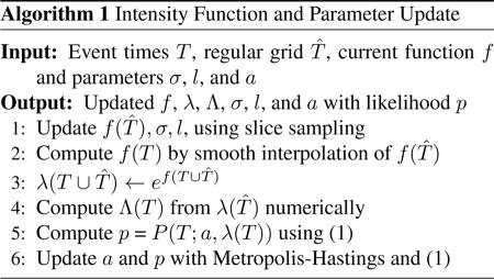
One challenge of this direct inference is that it requires integrating $\mathrm{\Lambda }(t)={\int }_0^t\lambda (u)du$, which is difficult because λ(t) does not have an explicit expression. Under certain conditions, the integral of a Gaussian process has a closed form (Rasmussen and Gharamani, 2003), but we know of no closed form for the integral of a log Gaussian process. Instead, we compute the integral numerically (the trapezoidal rule works fine), relying on the smoothness guarantees provided by the covariance function (3) to provide high accuracy.

The efficiency bottleneck of the update is the O(m³) complexity of updating the Gaussian process f at m locations, due to a matrix inversion. Naively, we would compute f at all n of the observed t_i, with additional points as needed for accuracy of the integral. To improve efficiency, we do not directly update f at the t_i, but instead at k uniformly spaced points T̂ = {t̂_j = t_min + jd}, where $d=\frac{t_{max}-t_{min}}{k-1}$. We then interpolate the values f(T) from the values of f(T̂) as needed. We set the number of points k by the accuracy required for the integral. This is driven by our estimate of the smallest likely Gaussian process time scale l_min, at which point we truncate the prior on l to guarantee d ≪ l_min ≤ l. The efficiency of the resulting update is O(k³)+O(n), with k depending only on the ratio l_min/(t_max − t_min).

It helps that the factor driving k is the time scale of changes in the intensity function λ(t) instead of the time scale of interevent intervals, which is usually much smaller. In practice, we’ve found k = 200 to work well for nearly all of our medical data examples, regardless of the observation time span, resulting in an update that is linear in the number of observed points.

Additionally, the regular spacing in T̂ means that its covariance matrix generated by (3) is a symmetric positive definite Toeplitz matrix, which can be inverted or solved in a compact representation as fast as O(k log² k) (Martinsson et al., 2005). We did not include this extra efficiency in our implementation, however.

3 RELATED WORK

There is a growing literature on finding patterns among clinical variables such as laboratory tests that have both a timestamp and a numeric value (Lasko et al., 2013), but we are not aware of any existing work exploring unsupervised, data-driven abstractions of categorical clinical event streams that we address here.

There is much prior work on methods similar to ours that infer intensity functions for modulated renewal processes. The main distinction between these methods lies in the way they handle the form and integration of the intensity function λ(t). Approaches include using kernel density estimation (Ramlau-Hansen, 1983), using parametric intensity functions (Lewis, 1972), using discretized bins within which the intensity is considered constant (Moller et al., 1998, Cunningham et al., 2008), or using a form of rejection sampling called thinning (Adams et al., 2009, Rao and Teh, 2011) that avoids the integration altogether.

The binned time approach is straightforward, but there is inherent information loss in the piecewise-constant intensity approximation that it must adopt. Moreover, when a Gaussian process is used to represent this intensity function, the computational complexity of inference is cubic with the number of bins in the interval of observation. For our data, with events at 1-day or finer time resolution over up to a 15 year observation period, this method is prohibitively inefficient. A variant of the binned-time approach that uses variable-sized bins (Gunawardana et al., 2011, Parikh et al., 2012) has been applied to medical data (Weiss and Page, 2013). This variant is very efficient, but is restricted to a Poisson process (fixed a = 1), and the inferred intensity functions are neither intended to nor particularly well suited to form an accurate abstraction over the raw events.

Thinning is a clever method, but it is limited by the requirement of a bounded hazard function, which prevents it from being used with bursty gamma processes. (Bursty gamma processes have a hazard function that is unbounded at zero). One thinning method has also adopted the use of Gaussian processes to modulate gamma processes (Rao and Teh, 2011). But in addition to not working with bursty events, it also rather inefficient; its time complexity is cubic in the number of events that would occur if the maximum event intensity were constant over the entire observation time span. For event streams with a small dynamic range of intensities, this is not a big issue, but our medical data sequences can have a dynamic range of several orders of magnitude.

Our method therefore has efficiency and flexibility advantages over existing methods, and we will demonstrate in the experiments that it also has accuracy advantages.

4 EXPERIMENTS

In these experiments, we will refer to our inference method as the direct method because it uses direct numerical integration. A full implementation of our method and code to reproduce the results on the synthetic data is available at https://github.com/ComputationalMedicineLab/egpmrp.

We tested the ability of the direct method and the thinning method to recover known intensity functions and shape parameters from synthetic data. We then used the direct method to extract latent intensity functions from streams of clinical events, and we inferred latent compound conditions from the intensity functions for a complex patient record that accurately correspond to the dominant diseases documented in the record.

4.1 SYNTHETIC DATA

Our first experiments were with the three parametric intensity functions below, carefully following Adams et al. (2009) and Rao and Teh (2011). We generated all data using the warping model described in Section 2, with shape parameter a = 3.

1. λ₁(t)/a = 2e^−t/15 + e^{−((t−25)/10)2} over the interval [0, 50], 48 events.

2. λ₂(t)/a = 5 sin(t²) + 6 on [0, 5], 29 events.

3. λ₃(t)/a is the piecewise linear curve shown in Figure 1, on the interval [0, 100], 230 events.

Figure 1.

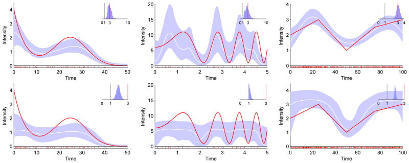
Our direct method (top) is more accurate than thinning (bottom) on parametric intensity functions λ₁ to λ₃ (left to right). Red line: true normalized intensity function λ(t)/a; White line: mean inferred normalized intensity function; Blue region: 95% confidence interval. Inset: inferred distribution of the gamma shape parameter a, with the true value marked in red. Grey bar at a = 1 for reference.

We express these as normalized intensities λ(t)/a, which have units of “expected number of events per unit time”, because they are more interpretable than the raw intensities and they are comparable to the previous work done using Poisson processes, where a = 1.

We compared the direct method to thinning on these datasets, using the MATLAB implementation for thinning that was used by Rao and Teh (2011). Adams et al. (2009) compared thinning to the kernel smoothing and binned time methods (all assuming a Poisson process), and Rao and Teh (2011) compared thinning to binned time, assuming a gamma process with constrained a > 1. Both found thinning to be at least as accurate as the other methods in most tests.

We computed the RMS error of the true vs. the median normalized inferred intensity, the log probability of the data given the model, and the inference run time under 1000 burn-in and 5000 inference MCMC iterations.

On these datasets the direct method was more accurate than thinning for the recovery of both the intensity function and the shape parameter, and more efficient by up to two orders of magnitude (Figure 1 and Table 1). The results for thinning are consistent with those previously reported (Rao and Teh, 2011), with the exception that the shape parameter inference was more accurate in the earlier results.

Table 1.

Performance on Synthetic Data. RMS: root-mean-squared error; LP: log probability of data given the model; RT: run time in seconds. Best results for each measure are bolded.

	Direct			Thinning
	RMS	LP	RT	RMS	LP	RT
λ1	0.37	+12.1	453	0.66	−62.7	4816
λ2	3.1	−228	511	3.4	−333	1129
λ3	0.25	+1.21	385	0.53	−82.2	41291

The confidence intervals from the direct method are subjectively more accurate than from the thinning method. (That is, the 95% confidence intervals from the direct method contain the true function for about 95% of its length in each case). This is particularly important in the case of small numbers of events that may not carry sufficient information for any method to resolve a highly varying function.

As might be expected, we found the results for λ₂(t) to be sensitive to the prior distribution on l, given the small amount of evidence available for the inference. Following Adams et al. (2009) and Rao and Teh (2011), we used a log-normal prior with a mode near l = 0.2, tuned slightly for each method to achieve the best results. We also allowed thinning to use a log-normal prior with appropriate modes for λ₁(t) and λ₃(t), to follow precedent in the previous work, although it may have conferred a small advantage to thinning. We used the weaker exponential prior on those datasets for the direct method.

Our next experiments were on synthetic data generated to resemble our medical data. We tested several configurations over wide ranges of parameters, including some that were not amenable to any known existing approach (such as the combination of a < 1, high dynamic range of intensity, and high ratio of observation period to event resolution, Figure 2). The inferred intensities and gamma parameters were consistently accurate. Estimates of the confidence intervals were also accurate, including in cases with low intensities and few events (Figure 2, right panel).

Figure 2.

Accurate recovery of intensity function and parameters under conditions that would be prohibitive for any other method of which we are aware. Left panel presents results for high intensities and many events, right panel for low intensities and few events. While there is insufficient evidence in the right panel to recover the true intensity, the inferred intensity is reasonable given the evidence, and the inferred confidence intervals are accurate in that the true intensity is about 95% contained within them. Legend as in Figure 1.

4.2 CLINICAL DATA

We applied the direct method to sequences of billing codes representing clinical events. After obtaining IRB approval, we extracted all ICD-9 codes from five patient records with the greatest number of such codes in the deidentified mirror of our institution’s Electronic Medical Record. We arranged the codes from each patient record as streams of events grouped at the top (or chapter) level of the ICD-9 disease hierarchy (which collects broadly related conditions), as well as at the level of the individual disease.

For the streams of grouped events, we included an event if its associated ICD-9 code fell within the range of the given top-level division. For example, any ICD-9 event with a code in the range [390 – 459.81] was considered a Cardiovascular event. While intensity functions are only strictly additive for Poisson processes, we still find the curves of grouped events to be informative.

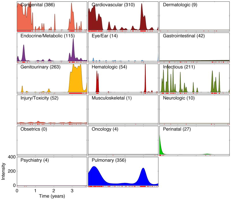
We inferred intensity functions for each of these event streams (for example, Figure 3). Each curve was generated using 2000 burn-in and 2000 inference iterations in about three minutes using unoptimized MATLAB code on a single desktop CPU. The results have good clinical face validity.

Figure 3.

Inferred intensities for all top-level ICD-9 disease divisions of a very complicated patient’s record. Such a display may be clinically useful for getting a quick, broad understanding of a patient’s medical history, including quickly grasping which conditions have not been diagnosed or treated. Numbers in parentheses: total number of events in each division. For clarity, confidence intervals are not shown.

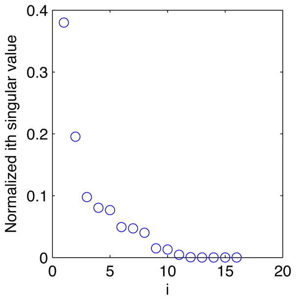
There is much underlying structure in these events that can now be investigated with standard learning methods applied to the inferred intensity functions. As a simple example, singular value decomposition (Strang, 2003) can infer the latent compound conditions (which we might as well call eigendiseases) underlying the recorded clinical activity, taking into account the continuously changing, longitudinal time course of that activity. The singular values for the curves in Figure 3 reveal that about 40% of the patient’s activity relates to a single eigendisease, and about 70% is distributed among the top three (Figure 4). The inferred eigendiseases closely correspond to the dominant clinical problems described in the record (Figure 5).

Figure 4.

A small number of latent compound conditions (or eigendiseases) produce most of the activity captured by the patient record in Figure 3.

Figure 5.

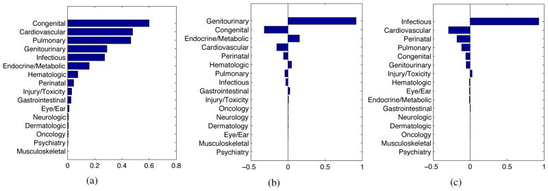
The top three eigendiseases inferred from the patient record in Figure 3. These align well with the actual clinical problems described in the record, which are a) severe congenital malformation of the heart and lungs with downstream effects on multiple organ systems, b) non-congenital kidney failure (a genitourinary condition with metabolic consequences), and c) multiple recurring infections from several sources.

5 DISCUSSION

We have made two contributions with this paper. First, we presented a direct numeric method to infer a distribution of continuous intensity functions from a set of episodic, irregular, and discrete events. This direct method has increased efficiency, flexibility, and accuracy compared to the best prior method. Second, we presented results using the direct method to infer a continuous function density as an abstraction over episodic clinical events, for the purposes of transforming the raw event data into a form more amenable to standard machine learning algorithms.

The clinical interpretation of these intensity functions is that increased intensity represents increased frequency of contact with the healthcare system, which usually means increased instability of that condition. In some cases, it may also mean increased severity of the condition, but not always. If a condition acutely increases in severity, this represents an instability and will probably generate a contact event. On the other hand, if a condition is severe but stably so, it may not necessarily require high-frequency medical contact.

The methods described here to represent categorically labeled events in time as continuous curves augment our previously reported methods to construct similar curves from observations with both a time and a continuous value (Lasko et al., 2013). These two data types represent the majority of the information in a patient record (if we consider words and concepts in narrative text to be categorical variables), and opens up many possibilities for finding meaningful patterns in large medical datasets.

The practical motivation for this work is that once we have the continuous function densities, we can use them as inputs to a learning problem in the time domain (such as identifying trajectories that may be characteristic of a particular disease), or by aligning many such curves in time and looking for useful patterns in their cross-sections (which to our knowledge has not yet been reported). We presented a simple demonstration of inferring cross-sectional latent factors from the intensity curves of a single record. Discovering similar latent factors underlying a large population is a focus of future work.

We discovered incidentally that a presentation such as Figure 3 appears to be a promising representation for efficiently summarizing a complicated patient’s medical history and communicating that broad summary to a clinician. The presentation could allow drilling-down to the intensity plots of the specific component conditions and then to the raw source data. (The usual method of manually paging through the often massive chart of a patient to get this information can be a tedious and frustrating process.)

One could also imagine presenting the curves not of the raw ICD-9 codes, but of the inferred latent factors underlying them, and drilling down into the rich combinations of test results, medications, narrative text, and discrete billing events that comprise those latent factors.

We believe that these methods will facilitate Computational Phenotype Discovery (Lasko et al., 2013), or the data-driven search for population-scale clinical patterns in existing electronic medical records that may illuminate previously unknown disease variants, unanticipated medication effects, or emerging syndromes and infectious disease outbreaks.

References

- Adams RP, Murray I, MacKay DJC. Tractable nonparametric Bayesian inference in Poisson processes with Gaussian process intensities. Proceedings of the 26th International Conference on Machine Learning; 2009. [Google Scholar]
- Berman M. Inhomogeneous and modulated gamma processes. Biometrika. 1981;68(1):143– 152. [Google Scholar]
- Cunningham JP, Yu BM, Shenoy KV. Inferring neural firing rates from spike trains using gaussian processes. Advances in Neural Information Processing Systems. 2008 [Google Scholar]
- Gunawardana A, Meek C, Xu P. A model for temporal dependencies in event streams. Advances in Neural Information Processing Systems. 2011 [Google Scholar]
- Lasko TA, Denny JC, Levy MA. Computational phenotype discovery using unsupervised feature learning over noisy, sparse, and irregular clinical data. PLoS One. 2013;8(6):e66341. doi: 10.1371/journal.pone.0066341. [DOI] [PMC free article] [PubMed] [Google Scholar]
- Lewis PAW. Recent results in the statistical analysis of univeraite point processes. In: Lewis PAW, editor. Stochastic Point Processes; Statistical Analysis, Theory, and Applications. Wiley Interscience; 1972. [Google Scholar]
- Martinsson P, Rokhlin V, Tygert M. A fast algorithm for the inversion of general toeplitz matrices. Computers & Mathematics with Applications. 2005;50(5–6):741–752. [Google Scholar]
- Moller J, Syversveen AR, Waagepetersen RP. Log gaussian cox processes. Scand J Stat. 1998;25(3):451–482. [Google Scholar]
- Murray I, Adams RP. Slice sampling covariance hyperparameters of latent Gaussian models. In: Lafferty J, Williams CKI, Zemel R, Shawe-Taylor J, Culotta A, editors. Advances in Neural Information Processing Systems. 2010. [Google Scholar]
- Parikh AP, Gunawardana A, Meek C. Conjoint modeling of temporal dependencies in event streams. UAI Bayesian Modelling Applications Workshop; 2012. [Google Scholar]
- Ramlau-Hansen H. Smoothing counting process intensities by means of kernel functions. The Annals of Statistics. 1983;11(2):453– 466. [Google Scholar]
- Rao V, Teh YW. Gaussian process modulated renewal processes. Advances In Neural Information Processing Systems. 2011 [Google Scholar]
- Rasmussen CE, Gharamani Z. Bayesian monte carlo. Advances in Neural Information Processing Systems. 2003 [Google Scholar]
- Strang G. Introduction to Linear Algebra. 7. 3. Vol. 6. Wellesley-Cambridge; Wellesley, MA: 2003. Singular value decomposition (SVD) pp. 352–362. [Google Scholar]
- Weiss JC, Page D. Forest-based point process for event prediction from electronic health records. In: Blockeel H, Kersting K, Nijssen S, Felezn, editors. Machine Learning and Knowledge Discovery in Databases, volume 8190 of Lecture Notes in Computer Science. Springer; Berlin Heidelberg: 2013. pp. 547–562. [Google Scholar]