The PREDICTS database: a global database of how local terrestrial biodiversity responds to human impacts

Abstract

Biodiversity continues to decline in the face of increasing anthropogenic pressures such as habitat destruction, exploitation, pollution and introduction of alien species. Existing global databases of species’ threat status or population time series are dominated by charismatic species. The collation of datasets with broad taxonomic and biogeographic extents, and that support computation of a range of biodiversity indicators, is necessary to enable better understanding of historical declines and to project – and avert – future declines. We describe and assess a new database of more than 1.6 million samples from 78 countries representing over 28,000 species, collated from existing spatial comparisons of local‐scale biodiversity exposed to different intensities and types of anthropogenic pressures, from terrestrial sites around the world. The database contains measurements taken in 208 (of 814) ecoregions, 13 (of 14) biomes, 25 (of 35) biodiversity hotspots and 16 (of 17) megadiverse countries. The database contains more than 1% of the total number of all species described, and more than 1% of the described species within many taxonomic groups – including flowering plants, gymnosperms, birds, mammals, reptiles, amphibians, beetles, lepidopterans and hymenopterans. The dataset, which is still being added to, is therefore already considerably larger and more representative than those used by previous quantitative models of biodiversity trends and responses. The database is being assembled as part of the PREDICTS project (Projecting Responses of Ecological Diversity In Changing Terrestrial Systems – www.predicts.org.uk). We make site‐level summary data available alongside this article. The full database will be publicly available in 2015.

The collation of biodiversity datasets with broad taxonomic and biogeographic extents is necessary to understand historical declines and to project – and hopefully avert – future declines. We describe a newly collated database of more than 1.6 million biodiversity measurements from 78 countries representing over 28,000 species, collated from existing spatial comparisons of local‐scale biodiversity exposed to different intensities and types of anthropogenic pressures, from terrestrial sites around the world.

Introduction

Despite the commitment made by the Parties to the Convention on Biological Diversity (CBD) to reduce the rate of biodiversity loss by 2010, global biodiversity indicators show continued decline at steady or accelerating rates, while the pressures behind the decline are steady or intensifying (Butchart et al. 2010; Mace et al. 2010). Evaluations of progress toward the CBD's 2010 target highlighted the need for datasets with broader taxonomic and geographic coverage than existing ones (Walpole et al. 2009; Jones et al. 2011). Taxonomic breadth is needed because species’ ability to tolerate human impacts – destruction, degradation and fragmentation of habitats, the reduction of individual survival and fecundity through exploitation, pollution and introduction of alien species – varies among major taxonomic groups (Vié et al. 2009). For instance, the proportion of species listed as threatened in the IUCN Red List is much higher in amphibians than in birds (International Union for Conservation of Nature 2013). Geographic breadth is needed because human impacts show strong spatial variation: most of Western Europe has long been dominated by human land use, for example, whereas much of the Amazon basin is still close to a natural state (Ellis et al. 2010). Thus, in the absence of broad coverage, any pattern seen in a dataset is prone to reflect the choice of taxa and region as much as true global patterns and trends.

The most direct way to capture the effects of human activities on biodiversity is by analysis of time‐series data from ecological communities, assemblages or populations, relating changes in biodiversity to changes in human activity (Vačkář 2012). However, long‐term data suitable for such modeling have limited geographic and taxonomic coverage, and often record only the presence or absence of species (e.g., Dornelas et al. 2013). Time‐series data are also seldom linked to site‐level information on drivers of change, making it hard to use such data to model biodiversity responses or to project responses into the future. Ecologists have therefore more often analyzed spatial comparisons among sites that differ in the human impacts they face. Although the underlying assumption that biotic differences among sites are caused by human impacts has been criticized (e.g., Johnson and Miyanishi 2008; Pfeifer et al. 2014), it is more likely to be reasonable when the sites being compared are surveyed in the same way, when they are well matched in terms of other potentially important variables (e.g., Blois et al. 2013; Pfeifer et al. 2014), when analyses focus on community‐level summaries rather than individual species (e.g., Algar et al. 2009), and when the spatial and temporal variations being considered are similar in magnitude (Blois et al. 2013). Collations of well‐matched site surveys therefore offer the possibility of analyzing how biodiversity is responding to human impacts without losing taxonomic and geographic breadth.

Openness of data is a further important consideration. The reproducibility and transparency that open data can confer offer benefits to all areas of scientific research, and are particularly important to research that is potentially relevant to policy (Reichman et al. 2011). Transparency has already been highlighted as crucial to the credibility of biodiversity indicators and models (e.g., UNEP‐WCMC 2009; Feld et al. 2010; Heink and Kowarik 2010) but the datasets underpinning previous policy‐relevant analyses have not always been made publicly available.

We present a new database that collates published, in‐press and other quality‐assured spatial comparisons of community composition and site‐level biodiversity from terrestrial sites around the world. The underlying data are made up of abundance, presence/absence and species‐richness measures of a wide range of taxa that face many different anthropogenic pressures. As of March 2014, the dataset contains more than 1.6 million samples from 78 countries representing over 28,000 species. The dataset, which is still being added to, is being assembled as part of the PREDICTS project (Projecting Responses of Ecological Diversity In Changing Terrestrial Systems – http://www.predicts.org.uk), the primary purpose of which is to model and project how biodiversity in terrestrial communities responds to human activity. The dataset is already considerably larger and more representative than those used in existing quantitative models of biodiversity trends such as the Living Planet Index (WWF International 2012) and GLOBIO3 (Alkemade et al. 2009).

In this paper we introduce the database, describe in detail how it was collated, validated and curated, and assess its taxonomic, geographic and temporal coverage. We make available a summary dataset that contains, for each sampling location, the predominant land use, land‐use intensity, type of habitat fragmentation, geographic coordinates, sampling dates, country, biogeographic realm, ecoregion, biome, biodiversity hotspot, taxonomic group studied and the number of measurements taken. The full dataset constitutes a large evidence base for the analysis of:

• The responses of biodiversity to human impacts for different countries, biomes and major taxonomic groups;

• The differing responses within and outside protected areas;

• How traits such as body size, range size and ecological specialism mediate responses and

• How human impacts alter community composition.

The summary dataset permits analysis of geographic and taxonomic variation in study size and design. The complete database, which will be made freely available at the end of the current phase of the project in 2015, will be of use to all researchers interested in producing models of how biodiversity responds to human pressures.

Methods

Criteria for inclusion

We considered only data that met all of the following criteria:

• Data are published, in press or were collected using a published methodology;

• The paper or report presents data about the effect of one or more human activities on one or more named taxa, and where the degree of human activity differed among sampling locations and/or times;

• Some measure of overall biodiversity, or of the abundance or occurrence of the named taxa, was made at two or more sampling locations and/or times;

• Measurements within each data source were taken using the same sampling procedure, possibly with variation in sampling effort, at each site and time;

• The paper reported, or authors subsequently provided, geographical coordinates for the sites sampled.

One of the modeling approaches used by PREDICTS is to relate diversity measurements to remotely sensed data, specifically those gathered by NASA's Moderate Resolution Imaging Spectroradiometer (MODIS) instruments (Justice et al. 1998). MODIS data are available from early 2000 onwards so, after a short initial data collation stage, we additionally required that diversity sampling had been completed after the beginning of 2000.

Where possible, we also obtained the following (see Site characteristics, below, for more details):

• The identities of the taxa sampled, ideally resolved to species level;

• The date(s) on which each measurement was taken;

• The area of the habitat patch that encompassed each site;

• The maximum linear extent sampled at the site;

• An indication of the land use at each site, e.g. primary, secondary, cropland, pasture;

• Indications of how intensively each site was used by people;

• Descriptions of any transects used in sampling (start point, end point, direction, etc.);

• Other information about each site that might be relevant to modeling responses of biodiversity to human activity, such as any pressures known to be acting on the site, descriptions of agriculture taking place and, for spatially blocked designs, which block each site was in.

Searches

We collated data by running sub‐projects that investigated different regions, taxonomic groups or overlapping anthropogenic pressures: some focused on particular taxa (e.g., bees), threatening processes (e.g., habitat fragmentation, urbanization), land‐cover classes (e.g., comparing primary, secondary and plantation tropical forests), or regions (e.g., Colombia). We introduced the project and requested data at conferences and in journals (Newbold et al. 2012; Hudson et al. 2013). After the first six months of broad searching, we increasingly targeted efforts toward under‐represented taxa, habitat types, biomes and regions. In addition to articles written in English, we also considered those written in Mandarin, Spanish and Portuguese – languages in which one or more of our data compilers were proficient.

Data collection

To maximize consistency in how incoming data were treated, we developed customized metadata and data capture tools – a PDF form and a structured Excel file – together with detailed definitions and instructions on their usage. The PDF form was used to capture bibliographic information, corresponding author contact details and meta‐data such as the country or countries in which data were collected, the number of taxa sampled, the number of sampling locations and the approximate geographical center(s) of the study area(s). The Excel file was used to capture details of each sampling site and the diversity measurements themselves. The PDF form and Excel file are available in Supplementary Information. We wrote software that comprehensively validates pairs of PDF and Excel files for consistency; details are in the “Database” section.

Most papers that we considered did not publish all the information that we required; in particular, site coordinates and species names were frequently not published. We contacted authors for these data and to request permission to include their contributed data in the PREDICTS database. We used the insightly customer relationship management application (https://www.insightly.com/) to manage contact with authors.

Structure of data

We structured data into Data Sources, Studies, and Sites. The highest level of organization is the Data Source. A Data Source typically represents data from a single published paper, although in some cases the data were taken from more than one paper, from a non‐governmental organization report or from a PhD or MSc thesis. A Data Source contains one or more Studies. A Study contains two or more Sites, a list of taxa that were sampled and a site‐by‐species matrix of observations (e.g., presence/absence or abundance). All diversity measurements within a Study must have been collected using the same sampling method. For example, a paper might present, for the same set of Sites, data from pitfall traps and from Malaise traps. We would structure these data into a single Data Source containing two Studies – one for each trapping technique. It is therefore reasonable to directly compare observations within a Study but not, because of methodological differences, among Studies. Sometimes, the data presented in a paper were aggregates of data from multiple sampling methods. In these cases, provided that the same set of sampling methods was applied at each Site, we placed the data in a single Study.

We classified the diversity observations as abundance, occurrence or species richness. Some of the site‐by‐species matrices that we received contained empty cells, which we interpreted as follows: (1) where the filled‐in values in the matrix were all non‐zero, we interpreted blanks as zeros or (2) where some of the values in the matrix were zero, we took empty cells as an indication that the taxa concerned were not looked for at those Sites, and interpreted empty cells as missing values.

Where possible, we recorded the sampling effort expended at each Site and allowed the units of sampling effort to vary among Studies. For example, if transects had been used, the (Study‐level) sampling effort units might be meters or kilometers and the (Site‐level) sampling efforts might be the length of the transects. If pitfall traps had been used, the (Study‐level) sampling effort units might be “number of trap nights” and the (Site‐level) sampling efforts might be the number of traps used multiplied by the number of nights that sampling took place. Where possible, we also recorded an estimate of the maximum linear extent encompassed by the sampling at each Site – the distance covered by a transect, the distance between two pitfall traps or the greatest linear extent of a more complex sampling design (see Figure S1 in Supplementary Information for details).

Site characteristics

We recorded each Site's coordinates as latitude and longitude (WGS84 datum), converting where necessary from local grid‐based coordinate systems. Where precise coordinates for Sites were not available, we georeferenced them from maps or schemes available from the published sources or provided by authors. We converted each map to a semi‐transparent image that was georeferenced using either ArcGIS (Environmental Systems Research Institute (ESRI) 2011) or Google Earth (http://www.google.co.uk/intl/en_uk/earth/ ), by positioning and resizing the image on the top of ArcGIS Online World Imagery or Google Maps until we achieved the best possible match of mapped geographical features with the base map. We then obtained geographic coordinates using geographic information systems (GIS) for each Site center or point location. We also recorded authors’ descriptions of the habitat at each Site and of any transects walked.

For each Site we recorded the dates during which sampling took place. Not all authors presented precise sampling dates – some gave them to the nearest month or year. We therefore recorded the earliest possible start date, the latest possible end date and the resolution of the dates that were given to us. Where dates were given to the nearest month or year, we recorded the start and end dates as the earliest and latest possible day, respectively. For example, if the authors reported that sampling took place between June and August of 2007, we recorded the date resolution as “month,” the start of sampling as June 1, 2007 and end of sampling as August 31, 2007. This scheme meant that we could store sampling dates using regular database structures (which require that the year, month, and day are all present), while retaining information about the precision of sampling dates that were given to us.

We assigned classifications of predominant land use and land‐use intensity to each Site. Because of PREDICTS’ aim of making projections about the future of biodiversity under alternative scenarios, our land‐use classification was based on five classes defined in the Representative Concentration Pathways harmonized land‐use estimates (Hurtt et al. 2011) – primary vegetation, secondary vegetation, cropland, pasture and urban – with the addition of plantation forest to account for the likely differences in the biodiversity of natural forest and plantation forest (e.g., Gibson et al. 2011) and a “Cannot decide” category for when insufficient information was available. Previous work has suggested that both the biodiversity and community composition differ strongly between sites in secondary vegetation of different maturity (Barlow et al. 2007); therefore, we subdivided secondary vegetation by stage – young, intermediate, mature and (when information was lacking) indeterminate – by considering vegetation structure (not diversity). We used authors’ descriptions of Sites, when provided, to classify land‐use intensity as minimal, light or intense, depending on the land use in question, again with “Cannot decide” as an option for when information was lacking. A detailed description of how classifications are assigned is in the Supplementary section “Notes on assigning predominant land use and use intensity” and Tables S1 and S2.

Given the likely importance of these classifications as explanatory variables in modeling responses of biodiversity to human impacts, we conducted a blind repeatability study in which one person (the last author, who had not originally scored any Sites) rescored both predominant land use and use intensity for 100 Sites chosen at random. Exact matches of predominant land use were achieved for 71 Sites; 15 of the remaining 29 were “near misses” specified in advance (i.e., primary vegetation versus mature secondary; adjacent stages of secondary vegetation; indeterminate secondary versus any other secondary stage; and cannot decide versus any other class). Cohen's kappa provides a measure of inter‐rate agreement, ranging from 0 (agreement no better than random) to 1 (perfect agreement). For predominant land use, Cohen's kappa = 0.662 (if only exact agreement gets credit) or 0.721 (if near misses are scored as 0.5); values in the range 0.6–0.8 indicate “substantial agreement” (Landis and Koch 1977), indicating that our categories, criteria and training are sufficiently clear for users to score Sites reliably. Moving to use intensity, we found exact agreement for 57 of 100 Sites, with 39 of the remaining 43 being “near misses” (adjacent intensity classes, or cannot decide versus any other class), giving Cohen's kappa values of 0.363 (exact agreement only) or 0.385 (near misses scored as 0.5), representing “fair agreement” (Landis and Koch 1977); agreement is slightly higher among the 71 Sites for which predominant land use was matched (exact agreement in 44 of 71 Sites, kappa = 0.428, indicating “moderate agreement”: Landis and Koch 1977).

Where known, we recorded the number of years since conversion to the present predominant land use. If the Site's previous land use was primary habitat, we recorded the number of years since it was converted to the current land use. If the habitat was converted to secondary forest (clear‐felled forest or abandoned agricultural land), we recorded the number of years since it was converted/clear‐felled/abandoned. Where ranges were reported, we used mid‐range values; if papers reported times as “greater than N years” or “at least N years,” we recorded a value of N × 1.25. Based on previous work (Wilcove et al. 1986; Dickman 1987), we assigned one of five habitat fragmentation classes: (1) well within unfragmented habitat, (2) within unfragmented habitat but at or near its edge, (3) within a remnant patch (perhaps at its edge) that is surrounded by other habitats, (4) representative part of a fragmented landscape and (5) part of the matrix surrounding remnant patches. These are described and illustrated in Table S3 and Figure S2. We also recorded the area of the patch of predominant habitat within which the Site was located, where this information was available. We recorded a value of −1 if the patch area was unknown but large, extending far beyond the sampled Site.

Database

Completed PDF and Excel files were uploaded to a PostgreSQL 9.1 database (PostgreSQL Global Development Group, http://www.postgresql.org/) with the PostGIS 2.0.1 spatial extension (Refractions Research Inc, http://www.postgis.net/). The database schema is shown in Figure S3.

We wrote software in the Python programming language (http://www.python.org/) to perform comprehensive data validation; files were fully validated before their data were added to the database. Examples of lower level invalid data included missing values for mandatory fields, a negative time since conversion, a latitude given as 1° 61’, a date given as 32nd January, duplicated Site names and duplicated taxon names. Commonly encountered higher level problems included mistakes in coordinates, such as latitude and longitude swapped, decimal latitude and longitude incorrectly assembled from DD/MM/SS components, and direction (north/south, east/west) swapped round. These mistakes typically resulted in coordinates that plotted in countries not matching those given in the metadata and/or out to sea. The former was detected automatically by validation software, which required that the GIS‐matched country for each Site (see “Biogeographical coverage ” below) matched the country name entered in the PDF file for the Study; where a Study spanned several countries, we set the country name to “Multiple countries.” We visually inspected all Site locations on a map and compared them to maps presented in the source article or given to us by the authors, catching coordinates that were mistakenly out to sea and providing a check of accuracy.

Our database linked each Data Source to the relevant record in our Insightly contact management database. This allows us to trace each datum back to the email that granted permission for us to include it in our database.

Biogeographical coverage

In order to assess the data's geographical and biogeographical coverage, we matched each Site's coordinates to GIS datasets that were loaded into our database:

• Terrestrial Ecoregions of the World (The Nature Conservancy 2009), giving the ecoregion, biome and biogeographic realm;

• World Borders 0.3 (Thematic Mapping 2008), giving the country, United Nations (UN) region and UN subregion;

• Biodiversity Hotspots (Conservation International Foundation 2011).

Global GIS layers appear coarse at local scales and we anticipated that Sites on coasts or on islands could fall slightly outside the relevant polygons. Our software therefore matched Sites to the nearest ecoregion and nearest country polygons, and recorded the distance in meters to that polygon, with a value of zero for Sites that fell within a polygon; we reviewed Sites with non‐zero distances. The software precisely matched Sites to hotspot polygons. The relative coarseness of GIS polygons might result in small errors in our assessments of coverage (i.e., at borders between biomes, ecoregions and countries, and at the edges of hotspots) – we expect that these errors should be small in number and unbiased.

We also estimated the yearly value of total net primary production (TNPP) for biomes and five‐degree latitudinal belts, using 2010 spatial (0.1‐degree resolution) monthly datasets “NPP – Net Primary Productivity 1 month‐Terra/MODIS” compiled and distributed by NASA Earth Observations (http://neo.sci.gsfc.nasa.gov/view.php?datasetId=MOD17A2_M_PSN&year=2010). We used the NPP values (average for each month assimilation measured in grams of carbon per square meter per day) to estimate monthly and annual NPP. We then derived TNPP values by multiplying NPP values by the total terrestrial area for that ecoregion/latitudinal belt. We assessed the representativeness of land use and land‐use intensity combinations by comparing the proportion of Sites in each combination to a corresponding estimate of the proportion of total terrestrial area for 2005, computed using land‐use data from the HYDE historical reconstruction (Hurtt et al. 2011) and intensity data from the Global Land Systems dataset (van Asselen and Verburg 2012).

Taxonomic names and classification

We wanted to identify taxa in our database as precisely as possible and to place them in higher level groups, which required relating the taxonomic names presented in our datasets to a stable and authoritative resource for nomenclature. We used the Catalogue of Life (http://www.catalogueoflife.org/) for three main reasons. First, it provides broad taxonomic coverage. Second, Catalogue of Life publishes Annual Checklists. Third, Catalogue of Life provides a single accepted taxonomic classification for each species that is represented. Not all databases provide this guarantee; for example, Encyclopedia of Life (http://www.eol.org/) provides zero, one or more taxonomic classifications for each represented species. We therefore matched taxonomic names to the Catalogue of Life 2013 Annual Checklist (Roskov et al. 2013, henceforth COL).

There was large variation in the form of the taxonomic names presented in the source datasets, for example:

• A Latin binomial, with and without authority, year and other information;

• A generic name, possibly with a number to distinguish morphospecies from congenerics in the same Study (e.g., “Bracon sp. 1”);

• The name of a higher taxonomic rank such as family, order, class;

• A common name (usually for birds), sometimes not in English;

• A textual description, code, letter or number with no further information except an indication of some aspect of higher taxonomy.

Most names were Latin binomials, generic names or morphospecies names. Few binomials were associated with an authority – even when they were, time constraints mean that it would not have been practical to make use of this information. Many names contained typographical errors.

We represented each taxon by three different names: “Name entered,” “Parsed name,” and “COL query name.” “Name entered” was the name assigned to the taxon in the dataset provided to us by the investigators who collected the data. We used the Global Names Architecture's biodiversity package ( https://github.com/GlobalNamesArchitecture/biodiversity) to parse “Name entered” and extract a putative Latin binomial, which we assigned to both “Parsed name” and “COL query name.” For example, the result of parsing the name “Ancistrocerus trifasciatus Müll.” was “Ancistrocerus trifasciatus.” The parser treated all names as if they were scientific taxonomic names, so the result of parsing common names was not sensible: e.g. “Black and White Casqued Hornbill” was parsed as “Black and.” We expected that common names would be rare – where they did arise, they were detected and corrected as part of our curation process, which is described below. Other examples of the parser's behavior are shown in Table S4.

We queried COL with each “COL query name” and stored the matching COL ID, taxonomic name, rank and classification (kingdom, phylum, class, order, family, genus, species and infraspecies). We assumed that the original authors gave the most authoritative identification of species. Therefore, when a COL search returned more than one result, and the results were made up of one accepted name together with one or more synonyms and/or ambiguous synonyms and/or common names and/or misapplied names, our software recorded the accepted name. For example, COL returns three results for the salticid spider Euophrys frontalis – one accepted name and two synonyms.

When a COL search returned more than one result, and the results included zero or two or more accepted names, we used the lowest level of classification common to all results. For example, COL lists Notiophilus as an accepted genus in two beetle families – Carabidae and Erirhinidae. This is a violation of the rules of nomenclature, but taxonomic databases are imperfect and such violations are to be expected. In this case, the lowest rank common to both families is the order Coleoptera.

Curating names

We reviewed:

• Taxa that had no matching COL record;

• Taxa that had a result at a rank higher than species and a “Name entered” that was either a Latin binomial or a common name;

• Cases where the same “Parsed name” in different Studies linked to different COL records;

• Studies for which the lowest common taxonomic rank did not seem appropriate; for example, a Study of birds should have a lowest common taxonomic rank of class Aves or lower rank within Aves.

Where a change was required, we altered “COL query name”, recording the reason why the change was made, and reran the COL query. Sometimes, this curation step had to be repeated multiple times. In all cases, we retained the names given to us by the authors, in the “Name entered” and “Parsed name” columns.

Typographical errors were the most common cause for failed COL searches; for example, the hymenopteran Diphaglossa gayi was given as Diphaglosa gayi. Such errors were detected by visual inspection and by performing manual searches on services that perform fuzzy matching and suggest alternatives, such as Google and Encyclopedia of Life. In cases where “Parsed name” was a binomial without typographical errors but that was not recognized by COL, we searched web sites such as Encyclopedia of Life and The Plant List (http://www.theplantlist.org/) for synonyms and alternative spellings and queried COL with the results. Where there were no synonyms or where COL did not recognize the synonyms, we searched COL for just the genus. If the genus was not recognized by COL, we used the same web services to obtain higher level ranks, until we found a rank that COL recognized.

Some names matched COL records in two different kingdoms. For example, Bellardia, Dracaena and Ficus are all genera of plants and of animals. In such cases, we instructed our software to consider only COL records from the expected kingdom. We also constrained results when a name matched COL records in two different branches within the same kingdom; for example, considering the Notiophilus example given above – if the Study was of carabid beetles, we would instruct of software to consider only results within family Carabidae.

COL allows searches for common names. Where “Name entered” was a common name that was not recognized by COL, we searched web sites as described above and set “COL query name” to the appropriate Latin binomial.

Some studies of birds presented additional complications. Some authors presented taxon names as four‐letter codes that are contractions of common names (e.g., AMKE was used by Chapman and Reich (2007) to indicate Falco sparverius, American kestrel) or of Latin binomials (e.g., ACBA was used by Shahabuddin and Kumar (2007) to indicate Accipiter badius). Some of these codes are valid taxonomic names in their own right. For example, Shahabuddin and Kumar (2007) used the code TEPA to indicate the passerine Terpsiphone paradisi. However, Tepa is also a genus of Hemiptera. Left uncurated, COL recognized TEPA as the hemipteran genus and the Study consequently had a lowest common taxonomic rank of kingdom Animalia, not of class Aves or a lower rank within Aves, as we would expect. Some codes did not appear on published lists (e.g., http://www.birdpop.org/alphacodes.htm, http://www.pwrc.usgs.gov/bbl/manual/speclist.cfm, http://www.carolinabirdclub.org/bandcodes.html and http://infohost.nmt.edu/~shipman/z/nom/bbs.html) or in the files provided by the authors, either because of typographical errors, omissions or incomplete coverage. Fortunately, codes are constructed by following a simple set of rules – the first two letters of the genus and species of binomials, and a slightly more complex method for common names of North American birds (http://infohost.nmt.edu/~shipman/z/nom/bblrules.html). We cautiously reverse‐engineered unrecognized codes by following the appropriate rules and then searched lists of birds of the country concerned for possible matches. For example, we deduced from the Wikipedia list of birds of India (http://en.wikipedia.org/wiki/List_of_birds_of_India) that KEZE – used in a study of birds in Rajasthan, northwestern India (Shahabuddin and Kumar 2007) – most likely indicates Ketupa zeylonensis. Another problem is that collisions occur – the same code can apply to more than one taxon. For example, PEPT is the accepted code for Atalotriccus pilaris (pale‐eyed pygmy tyrant – http://www.birdpop.org/alphacodes.htm), a species that occurs in the Neotropics. The same code was used by the Indian study of Shahabuddin and Kumar (2007) to indicate Pernis ptilorhynchus (crested honey buzzard). We therefore reverse‐engineered bird codes on a case‐by‐case basis. Where a code could represent more than one species, we set “COL query name” as the lowest taxonomic rank common to all matching species.

Counting the number of species

It was not possible to precisely count the number of species represented in our database because of ambiguity inherent in the taxon names provided with the data. We estimated the number of species as follows. Names with a COL result at either species or infraspecies level were counted once per name. Names with a COL result resolved to higher taxonomic ranks were counted once per Study. To illustrate this scheme, consider the bat genus Eonycteris, which contains three species. Suppose that Study A sampled all three species and that the investigators could distinguish individuals as belonging to three separate species but could not assign them to named species, reporting them as Eonycteris sp. 1, Eonycteris sp. 2 and Eonycteris sp. 3. Study B also sampled all three species of Eonycteris and again reported Eonycteris sp. 1, Eonycteris sp. 2 and Eonycteris sp. 3. We would erroneously consider these taxa to be six different species. We did not attempt to determine how often, if at all, such inflation occurred.

In order to assess the taxonomic coverage of our data, we computed a higher taxonomic grouping for each taxon as: (1) order where class was Insecta or Entognatha; (2) class where phylum was Arthropoda (excluding Insecta), Chordata or Tracheophyta; otherwise 3) phylum. So the higher taxonomic group of a bee is order Hymenoptera (following rule 1), the higher taxonomic group of a wolf is class Mammalia (rule 2), and the higher taxonomic group of a snail is phylum Gastropoda (rule 3). For each higher taxonomic group, we compared the numbers of species in our database to the estimated number of described species presented by Chapman (2009). Some of the higher taxonomic groups that we computed did not directly relate to the groups presented by Chapman (2009) so, in order to compare counts, we computed Magnoliophyta as the sum of Magnoliopsida and Liliopsida; Gymnosperms as the sum of Pinopsida and Gnetopsida; Ferns and allies as the sum of Polypodiopsida, Lycopodiopsida, Psilotopsida, Equisetopsida and Marattiopsida; and Crustacea as Malacostraca.

For some of our analyses, we related taxonomic names to databases of species’ traits. To do this, we synthesized, for each taxon, a “Best guess binomial”:

• The COL taxon name if the COL rank was Species;

• The first two words of the COL taxon if the rank was Infraspecies;

• The first two words of “Parsed name” if the rank was neither Species nor Infraspecies and “Parsed name” contained two or more words;

• Empty in other cases.

This scheme meant that even though COL did not recognize all of the Latin binomials that were given to us, we could maximize matches between names in our databases with names in the species’ trait databases.

Results

Between March 2012 and March 2014, we collated data from 284 Data Sources, 407 Studies and 13,337 Sites in 78 countries and 208 (of 814) ecoregions (Fig. 1). The best‐represented UN‐defined subregions are North America (17.51% of Sites), Western Europe (14.14%) and South America (13.37%). As of March 31, 2014, the database contained 1,624,685 biodiversity samples – 1,307,947 of abundance, 316,580 of occurrence and 158 of species richness. The subregions with the most samples are Southeast Asia (24.66%), Western Europe (11.36%) and North America (10.88%).

Figure 1.

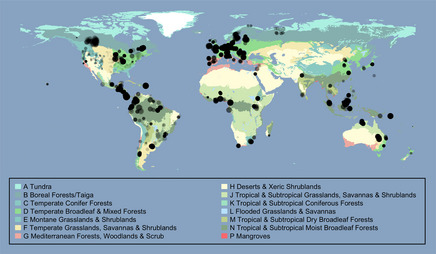
Site locations. Colors indicate biomes, taken from The Nature Conservancy's (2009) terrestrial ecoregions of the world dataset, shown in a geographic (WGS84) projection. Circle radii are proportional to log₁₀ of the number of samples at that Site. All circles have the same degree of partial transparency.

Of the world's 35 biodiversity hotspots, 25 are represented (Table 1). Hotspots together account for just 16% of the world's terrestrial surface, yet 47.67% of our measurements were taken in hotspots. The vast majority of measurements in hotspots were taken in the Sundaland hotspot (Southeast Asia) and the latitudinal band with the most samples is 0° to 5° N (Fig. 2); many of these data come from two studies of higher plants from Indonesia that between them contribute just 284 sites but over 320,000 samples (Sheil et al. 2002).

Table 1.

Coverage of hotspots.

Hotspot	Studies (%)	Sites (%)	Samples (%)	Terrestrial area (%)
None	50.72	63.63	52.33	84.01
Nearctic
California Floristic Province	0.96	1.30	0.12	0.20
Madrean Pine–Oak Woodlands	0.24	0.01	<0.01	0.31
Neotropic
Atlantic Forest	3.11	1.16	0.28	0.83
Caribbean Islands	0.48	0.67	2.59	0.15
Cerrado	1.91	0.66	0.11	1.37
Chilean Winter Rainfall and Valdivian Forests	2.39	1.69	0.32	0.27
Mesoamerica	8.13	7.83	8.94	0.76
Tropical Andes	6.46	3.02	4.11	1.04
Tumbes‐Choco‐Magdalena	0.48	0.37	0.10	0.18
Palearctic
Caucasus	0.00	0.00	0.00	0.36
Irano‐Anatolian	0.00	0.00	0.00	0.61
Japan	1.67	0.60	0.17	0.25
Mediterranean Basin	5.98	5.52	2.63	1.41
Mountains of Central Asia	0.00	0.00	0.00	0.58
Mountains of Southwest China	0.00	0.00	0.00	0.18
Afrotropic
Cape Floristic Region	0.24	0.29	0.20	0.05
Coastal Forests of Eastern Africa	0.00	0.00	0.00	0.20
Eastern Afromontane	1.20	1.27	0.83	0.07
Guinean Forests of West Africa	2.15	1.04	0.54	0.42
Horn of Africa	0.00	0.00	0.00	1.12
Madagascar and the Indian Ocean Islands	0.48	0.18	0.01	0.40
Maputaland–Pondoland–Albany	0.72	0.52	0.50	0.18
Succulent Karoo	0.00	0.00	0.00	0.07
Indo‐Malay
Himalaya	0.00	0.00	0.00	0.50
Indo‐Burma	0.72	0.23	0.10	1.60
Philippines	1.20	0.77	0.44	0.20
Sundaland	6.46	6.12	23.55	1.01
Western Ghats and Sri Lanka	0.48	0.13	0.09	0.13
Australasia
East Melanesian Islands	0.24	0.36	1.13	0.68
Forests of East Australia	0.72	1.45	0.31	0.17
New Caledonia	0.00	0.00	0.00	0.01
New Zealand	0.72	0.10	0.01	0.18
Southwest Australia	0.00	0.00	0.00	0.24
Wallacea	1.67	0.69	0.58	0.23
Oceania
Polynesia–Micronesia	0.48	0.38	0.01	0.03

Hotspots are shown grouped by realm.

Figure 2.

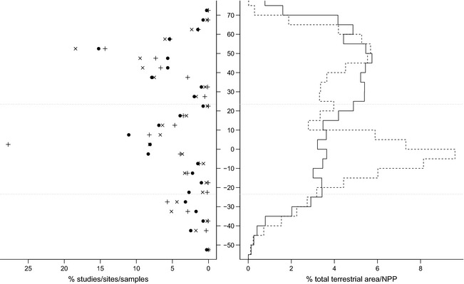
Latitudinal coverage. The percentage of Studies (circles), Sites (crosses) and samples (pluses) in five‐degree bands of latitude. We computed each Study's latitude as the median of its Sites’ latitudes. The solid and dashed lines show the percentage of total terrestrial area and percentage of total terrestrial NPP, respectively, in each five‐degree band (see “ Biogeographical coverage ” in Methods). The dotted horizontal lines indicate the extent of the tropics.

The best‐represented biomes are “Temperate Broadleaf and Mixed Forests” and “Tropical and Subtropical Moist Broadleaf Forests” (Figs 3, 4). “Flooded Grasslands and Savannas” is the only biome that is unrepresented in our database (Figs 3, 4); although this biome is responsible for only 0.7% of global terrestrial net primary productivity, it is nevertheless ecologically important and will be a priority for future collation efforts. Two biomes – “Tundra” and “Deserts and Xeric Shrublands” – are underrepresented relative to their areas. Of the world's 17 megadiverse countries identified by Mittermeier et al. (1997), only Democratic Republic of Congo is not represented (Figure S4). The vast majority of sampling took place after the year 2000 (Fig. 3), reflecting our desire to collate diversity data that can be related to MODIS data, which are available from early 2000 onwards. The database's coverage of realms, biomes, countries, regions and subregions is shown in Supplementary Tables S5–S11.

Figure 3.

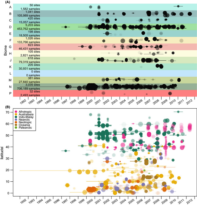
Spatiotemporal sampling coverage. Site sampling dates by biome (A) and absolute latitude (B). Each Site is represented by a circle and line. Circle radii are proportional to log₁₀ of the number of samples at that Site. Circle centers are at the midpoints of Site sampling dates; lines indicate the start and end dates of sampling. Y‐values in (A) have been jittered at the study level. Circles and lines have the same degree of partial transparency. Biome colors and letters in (A) are as in Fig. 1. Colors in (B) indicate biogeographic realm.

Figure 4.

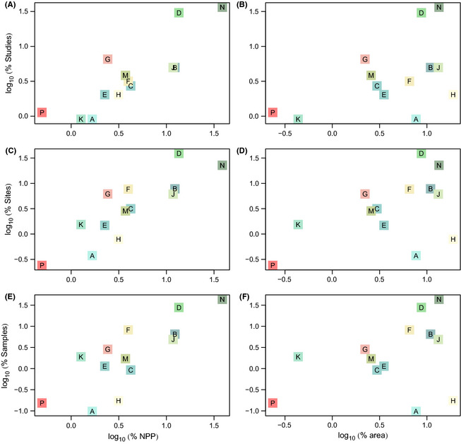
Coverage of biomes. The percentage of Studies (A and B), Sites (C and D) and samples (E and F) against percentages of terrestrial NPP (A, C and E) and terrestrial area (B, D and F). Biome colors and letters are as in Fig. 1.

The distribution of Site‐level predominant land use and use intensity is different from the distribution of the estimated total terrestrial area in each land use/land‐use intensity combination for 2005 (χ2 = 28,243.21, df = 16, P < 2.2 × 10⁻¹⁶; we excluded “Urban”/”Light use” from this test because the HYDE and Global Land Systems datasets did not allow us to compute an estimate for this combination). The main discrepancies are that the database has far fewer than expected Sites that are classified as “Primary habitat”/“Minimal use”, “Secondary vegetation”/“Light use” and “Pasture”/“Light use” (Fig. 5). We were unable to assign a classification of predominant land use to 3.34% of Sites and of use intensity to 12.09% of Sites. The most common fragmentation layout was “Representative part of a fragmented landscape” (27.95% of Sites; Table S12) – a classification that indicates either that a Site is large enough to encompass multiple habitat types or that the Site is of a particular habitat type that is inherently fragmented and dominates the landscape e.g., the site is in an agricultural field and the landscape is comprised of many fields. We were unable to assign a fragmentation layout to 15.47% of Sites. We were able to determine the maximum linear extent of sampling for 60.09% of Sites – values range from 0.2 m to 39.15 km; median 120 m (Figure S5). The precise sampling days are known for 45.44% of Sites; 42.19% are known to the nearest month and 12.37% to the nearest year. The median sampling duration was 91 days; sampling lasted for 1 day or less at 9.90% of Sites (Figure S6). The area of habitat containing the site is known for 25.49% of Sites – values are approximately log‐normally distributed (median 40,000 square meters; Figure S7). We reviewed all cases of Sites falling outside the GIS polygons for countries (0.82% of Sites; Figure S8) and ecoregions (0.52% of Sites; Figure S9). These Sites were either on coasts and/or on islands too small to be included in the GIS dataset in question.

Figure 5.

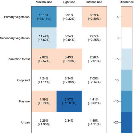
Representativeness of predominant land use and land‐use intensity classes. Numbers are the percentage of Sites assigned to each combination of land use and intensity. Numbers in brackets and colors are the differences between these and the proportional estimated total terrestrial area of each combination of land use and land‐use intensity for 2005, computed from the HYDE (Hurtt et al. 2011) and Global Land Systems datasets (van Asselen and Verburg 2012); no difference is shown for “Urban”/”Light use” because these datasets did not allow us to compute an estimate for this combination. The 12.15% of Sites that could not be assigned a classification for predominant land use and/or land‐use intensity are not shown.

The database contains measurements of approximately 28,735 species (see “ Counting the number of species ” in Methods) – 17,733 animals, 10,201 plants, 800 fungi and 1 protozoan. We were unable to place 97 taxa in a higher taxonomic group because they were not sufficiently well resolved. The database contains more than 1% as many species as have been described within 20 higher taxonomic groups (Fig. 6). Birds are particularly well represented, reflecting the sampling bias in favor of this charismatic group. Our database contains measurements of 2,479 species of birds – 24.81% of those described (Chapman 2009) – and 2,368 of these are resolved to either species or infraspecies levels. A total of 228,644 samples – more than 14% of the entire database – are of birds. In contrast, just 397 species of mammals are represented, but even this constitutes 7.24% of described species. Chiroptera (bats) are the best‐represented mammalian order with 188 species. Of the 115,000 estimated described species of Hymenoptera, 3,556 (3.09%) are represented in the database, the best representation of an invertebrate group. The hymenopteran family with the most species in the database is Formicidae with 2,060 species. The database contains data for 4,056 species of Coleoptera – 1.07% of described beetles. Carabidae is the best‐represented beetle family with 2,060 species. Some higher taxonomic groups have well below 1% representation and, as might be expected, the database has poor coverage of groups for which the majority of species are marine – nematodes, crustaceans and molluscs.

Figure 6.

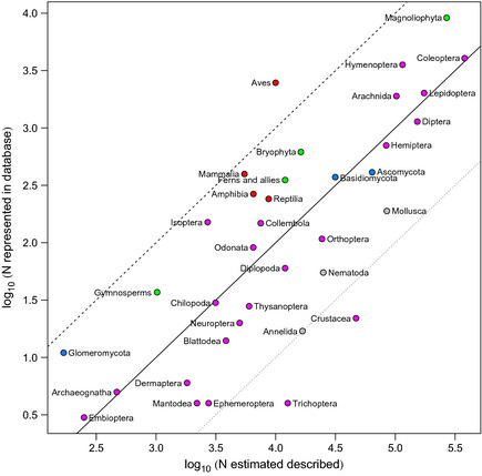
Taxonomic coverage. The number of species in our database against the number of described species as estimated by Chapman (2009). Vertebrates are shown in red, arthropods in pink, other animals in gray, plants in green and fungi in blue. The dashed, solid and dotted lines indicate 10, 1 and 0.1% representation, respectively. Groups with just a single species in the database – Diplura, Mycetozoa, Onychophora, Pauropoda, Phasmida, Siphonaptera, Symphyla and Zoraptera – are not shown.

Of the 28,735 species, 43.26% are matched to a COL record with a rank of species or infraspecies, 37.47% to a COL record with a rank of genus and 19.27% to a COL record with a higher taxonomic rank (Fig. 7). The species with the largest number of measurements – 1,305 – is Bombus pascuorum (the common carder bee), and bees constitute 35 of the top 100 most frequently sampled species: this results from a PREDICTS subproject that is examining pollinators. Birds make up most of the remaining top 100, with 36 species. Of the 407 Studies, 126 sampled within a single order (Fig. 8); just 12 Studies examined a single species. The six most commonly examined higher taxonomic groups are Tracheophyta (12.04% of Studies), Aves (11.06%), Hymenoptera (7.86%), Arthropoda (4.67%), Formicidae (4.67%) and Insecta (4.42%). The database contains 17,802 unique values of “Best guess binomial”. The overlap with species attribute databases is often much higher than would be expected by chance (Table 2), greatly facilitating analyses that integrate PREDICTS data with species attributes (Newbold et al. 2013, 2014a).

Figure 7.

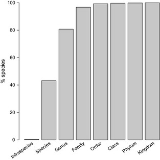
Cumulative percentage of species in the database, by the taxonomic rank at which the name was matched to COL.

Figure 8.

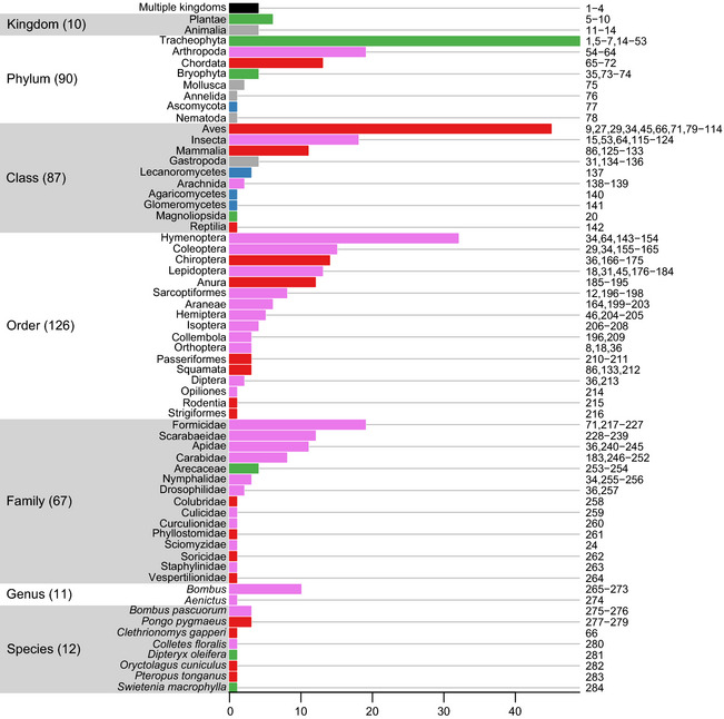
Number of Studies by lowest common taxonomic group. Bars show the number of Studies within each lowest common taxon (so, one Study examined the species Swietenia macrophylla, three Studies examined the species Bombus pascuorum, ten Studies examined multiple species within the genus Bombus, and so on). Colors are as in Figure 6. Numbers on the right are the primary references from which data were taken: 1 López‐Quintero et al. 2012; 2 Buscardo et al. 2008; 3 Domínguez et al. 2012; 4 Nöske et al. 2008; 5 Center for International Forestry Research (CIFOR) 2013a; 6 Center for International Forestry Research (CIFOR) 2013b; 7 Sheil et al. 2002; 8 Dumont et al. 2009; 9 Proenca et al. 2010; 10 Baeten et al. 2010a, b; 11 Richardson et al. 2005; 12 Schon et al. 2011; 13 Muchane et al. 2012; 14 Vázquez and Simberloff 2002; 15 Bouyer et al. 2007; 16 O'Connor 2005; 17 Higuera and Wolf 2010; 18 Kati et al. 2012; 19 Lucas‐Borja et al. 2011; 20 Louhaichi et al. 2009; 21 Power et al. 2012; 22 Brearley 2011; 23 Baeten et al. 2010a; 24 Williams et al. 2009; 25 Mayfield et al. 2006; 26 Kolb and Diekmann 2004; 27 Phalan et al. 2011; 28 Vassilev et al. 2011; 29 Paritsis and Aizen 2008; 30 Boutin et al. 2008; 31 Baur et al. 2006; 32 Fensham et al. 2012; 33 Brunet et al. 2011; 34 Kessler et al. 2009; 35 Hylander and Nemomissa 2009; 36 Barlow et al. 2007; 37 Kumar and Shahabuddin 2005; 38 Kessler et al. 2005; 39 Hietz 2005; 40 Krauss et al. 2004; 41 Hernández et al. 2012; 42 Calviño‐Cancela et al. 2012; 43 Golodets et al. 2010; 44 Castro et al. 2010; 45 Milder et al. 2010; 46 Helden and Leather 2004; 47 McNamara et al. 2012; 48 Katovai et al. 2012; 49 Berry et al. 2010; 50 Letcher and Chazdon 2009; 51 Romero‐Duque et al. 2007; 52 Marin‐Spiotta et al. 2007; 53 Power and Stout 2011; 54 Norfolk et al. 2012; 55 Poveda et al. 2012; 56 Cabra‐García et al. 2012; 57 Turner and Foster 2009; 58 Woodcock et al. 2007; 59 Lachat et al. 2006; 60 Rousseau et al. 2013; 61 Nakamura et al. 2003; 62 Basset et al. 2008; 63 Hanley 2011; 64 Billeter et al. 2008; Diekötter et al. 2008; Le Féon et al. 2010; 65 Sung et al. 2012; 66 St‐Laurent et al. 2007; 67 Centro Agronómico Tropical de Investigación y Enseñanza (CATIE) 2010; 68 Endo et al. 2010; 69 Alcala et al. 2004; 70 Bicknell and Peres 2010; 71 Woinarski et al. 2009; 72 Garden et al. 2010; 73 Hylander and Weibull 2012; 74 Giordano et al. 2004; 75 Ström et al. 2009; 76 Römbke et al. 2009; 77 Giordani 2012; 78 Hu and Cao 2008; 79 Edenius et al. 2011; 80 O'Dea and Whittaker 2007; 81 Ims and Henden 2012; 82 Rosselli 2011; 83 Arbeláez‐Cortés et al. 2011; 84 Santana et al. 2012; 85 Sheldon et al. 2010; 86 Wang et al. 2010; 87 Sodhi et al. 2010; 88 Naoe et al. 2012; 89 Cerezo et al. 2011; 90 Lantschner et al. 2008; 91 Chapman and Reich 2007; 92 Báldi et al. 2005; 93 Farwig et al. 2008; 94 Shahabuddin and Kumar 2007; 95 Borges 2007; 96 Wunderle et al. 2006; 97 Politi et al. 2012; 98 Moreno‐Mateos et al. 2011; 99 Mallari et al. 2011; 100 Latta et al. 2011; 101 Sosa et al. 2010; 102 Miranda et al. 2010; 103 Flaspohler et al. 2010; 104 Bóçon 2010; 105 Azpiroz and Blake 2009; 106 Aben et al. 2008; 107 Cockle et al. 2005; 108 Vergara and Simonetti 2004; 109 Azhar et al. 2013; 110 Reid et al. 2012; 111 Neuschulz et al. 2011; 112 Dawson et al. 2011; 113 Naidoo 2004; 114 Dures and Cumming 2010; 115 Meyer et al. 2009; 116 Summerville 2011; 117 Cleary et al. 2004; 118 Mudri‐Stojnic et al. 2012; 119 Schüepp et al. 2011; 120 Bates et al. 2011; 121 Quintero et al. 2010; 122 Vergara and Badano 2009; 123 Kohler et al. 2008; 124 Meyer et al. 2007, 125 Hoffmann and Zeller 2005; 126 Caceres et al. 2010; 127 Lantschner et al. 2012; 128 Wells et al. 2007; 129 Bernard et al. 2009; 130 Martin et al. 2012; 131 Gheler‐Costa et al. 2012; 132 Sridhar et al. 2008; 133 Scott et al. 2006; 134 Oke 2013; 135 Oke and Chokor 2009; 136 Kappes et al. 2012; 137 Walker et al. 2006; 138 Lo‐Man‐Hung et al. 2008; 139 Zaitsev et al. 2002; 140 Robles et al. 2011; 141 Brito et al. 2012; 142 Luja et al. 2008; 143 Smith‐Pardo and Gonzalez 2007; 144 Schüepp et al. 2012; 145 Tylianakis et al. 2005; 146 Verboven et al. 2012; 147 Osgathorpe et al. 2012; 148 Tonietto et al. 2011; 149 Samnegård et al. 2011; 150 Cameron et al. 2011; 151 Malone et al. 2010; 152 Marshall et al. 2006; 153 Shuler et al. 2005; 154 Quaranta et al. 2004; 155 Légaré et al. 2011; 156 Noreika 2009; 157 Otavo et al. 2013; 158 Numa et al. 2012; 159 Jonsell 2012; 160 Mico et al. 2013; 161 Rodrigues et al. 2013; 162 Sugiura et al. 2009; 163 Verdú et al. 2007; 164 Banks et al. 2007; 165 Elek and Lovei 2007; 166 Fukuda et al. 2009; 167 Castro‐Luna et al. 2007; 168 Shafie et al. 2011; 169 Struebig et al. 2008; 170 Threlfall et al. 2012; 171 Presley et al. 2008; 172 Willig et al. 2007; 173 MacSwiney et al. 2007; 174 Clarke et al. 2005; 175 Sedlock et al. 2008; 176 Verdasca et al. 2012; 177 D'Aniello et al. 2011; 178 Berg et al. 2011; 179 Summerville et al. 2006; 180 Hawes et al. 2009; 181 Cleary and Mooers 2006; 182 Krauss et al. 2003; 183 Ishitani et al. 2003; 184 Safian et al. 2011; 185 Furlani et al. 2009; 186 Isaacs‐Cubides and Urbina‐Cardona 2011; 187 Gutierrez‐Lamus 2004; 188 Adum et al. 2013; 189 Watling et al. 2009; 190 Pillsbury and Miller 2008; 191 Pineda and Halffter 2004; 192 Ofori‐Boateng et al. 2013; 193 de Souza et al. 2008; 194 Faruk et al. 2013; 195 Hilje and Aide 2012; 196 Alberta Biodiversity Monitoring Institute (ABMI) 2013; 197 Zaitsev et al. 2006; 198 Arroyo et al. 2005; 199 Paradis and Work 2011; 200 Buddle and Shorthouse 2008; 201 Kapoor 2008; 202 Alcayaga et al. 2013; 203 Magura et al. 2010; 204 Littlewood et al. 2012; 205 Kőrösi et al. 2012; 206 Oliveira et al. 2013; 207 Carrijo et al. 2009; 208 Reis and Cancello 2007; 209 Chauvat et al. 2007; 210 Otto and Roloff 2012; 211 Zimmerman et al. 2011; 212 Pelegrin and Bucher 2012; 213 Savage et al. 2011; 214 Bragagnolo et al. 2007; 215 Jung and Powell 2011; 216 Bartolommei et al. 2013; 217 Dominguez‐Haydar and Armbrecht 2010; 218 Armbrecht et al. 2006; 219 Hashim et al. 2010; 220 Schmidt et al. 2012; 221 Maeto and Sato 2004; 222 Bihn et al. 2008; 223 Delabie et al. 2009; 224 Fayle et al. 2010; 225 Gove et al. 2005; 226 Buczkowski and Richmond 2012; 227 Buczkowski 2010; 228 Noriega et al. 2012; 229 Navarro et al. 2011; 230 Noriega et al. 2007; 231 Horgan 2009; 232 Gardner et al. 2008; 233 da Silva 2011; 234 Silva et al. 2010; 235 Jacobs et al. 2010; 236 Slade et al. 2011; 237 Filgueiras et al. 2011; 238 Navarrete and Halffter 2008; 239 Davis and Philips 2005; 240 Parra‐H and Nates‐Parra 2007; 241 Fierro et al. 2012; 242 Nielsen et al. 2011; 243 Julier and Roulston 2009; 244 Winfree et al. 2007; 245 Hanley 2005; 246 Liu et al. 2012; 247 Gu et al. 2004; 248 Noreika and Kotze 2012; 249 Rey‐Velasco and Miranda‐Esquivel 2012; 250 Vanbergen et al. 2005; 251 Koivula et al. 2004; 252 Weller and Ganzhorn 2004; 253 Carvalho et al. 2010; 254 Aguilar‐Barquero and Jiménez‐Hernández 2009; 255 Fermon et al. 2005; 256 Ribeiro and Freitas 2012; 257 Gottschalk et al. 2007; 258 Cagle 2008; 259 Johnson et al. 2008; 260 Su et al. 2011; 261 Saldana‐Vazquez et al. 2010; 262 Nicolas et al. 2009; 263 Sakchoowong et al. 2008; 264 Yoshikura et al. 2011; 265 Hanley et al. 2011; 266 Connop et al. 2011; 267 Redpath et al. 2010; 268 Goulson et al. 2010; 269 Goulson et al. 2008; 270 Hatfield and LeBuhn 2007; 271 McFrederick and LeBuhn 2006; 272 Diekötter et al. 2006; 273 Darvill et al. 2004; 274 Matsumoto et al. 2009; 275 Knight et al. 2009; 276 Herrmann et al. 2007; 277 Ancrenaz et al. 2004; 278 Felton et al. 2003; 279 Knop et al. 2004; 280 Davis et al. 2010; 281 Hanson et al. 2008; 282 Ferreira and Alves 2005; 283 Luskin 2010; 284 Grogan et al. 2008.

Table 2.

Names represented in species attribute databases.

Attribute database	Trait	Group	Best guess binomials	Attribute database names	Species matches	Genus matches	Total matches
GBIF	Range size	All taxa	17,801		14,514		14,514
IUCN	Red list status	All taxa	17,801		3,521		3,521
CITES	CITES appendix	All taxa	17,801	20,094	467		467
PanTHERIA	Body mass	Mammalia	376	3,542	310	62	372
TRY	Seed mass	Plantae	6,924	26,107	2,017	2,820	4,837
TRY	Vegetative height	Plantae	6,924	2,822	772	768	1,540
TRY	Generative height	Plantae	6,924	9,911	1,633	2,546	4,179

GBIF (Global Biodiversity Information Facility, http://www.gbif.org/, queried 2014‐03‐31), IUCN (International Union for Conservation of Nature, http://www.iucn.org/, queried 2014‐03‐31), CITES (Convention on International Trade in Endangered Species of Wild Fauna and Flora, http://www.cites.org/, downloaded 2014‐01‐27), PanTHERIA (Jones et al. 2009), TRY (Kattge et al. 2011). Best guess binomials: the number of unique “Best guess binomials” in the PREDICTS database within that taxonomic group. Attribute database names: the number of unique binomials and trinomials for that attribute in attribute database. Species matches: the number of “Best guess binomials” that exactly match a record in the attribute database. Genus matches: the number of generic names in the PREDICTS database with a matching record in the attribute database (only for binomials for which there was not a species match). Total matches: sum of species matches and genus matches. We did not match generic names for GBIF range size, IUCN category or CITES appendix because we did not expect these traits to be highly conserved within genera.

Of the 284 Data Sources, 271 were taken from articles published in scientific peer‐reviewed journals; the rest came from unpublished data (5), internet databases (3), PhD theses (2), agency reports (1) and other sources (2). The vast majority – 273 (96.13%) – of Data Sources are taken from English articles; the remainder are in Mandarin (0.35%), Portuguese (1.06%) or Spanish (2.46%). 29.15% of Data Sources come from just four journals (Fig. 9): Biological Conservation (11.07%), Biodiversity and Conservation (8.86%), Forest Ecology & Management (5.17%) and Journal of Applied Ecology (4.06%). The Journal of Applied Ecology contributed many more Studies, Sites and samples than expected from the number of Data Sources (Fig. 9) because of a single Data Source that contributed 21 pan‐European Studies and over 140,000 samples (data taken from Billeter et al. 2008; Diekötter et al. 2008 and Le Féon et al. 2010).

Figure 9.

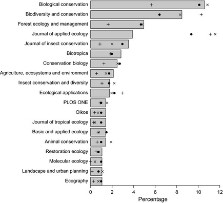
Data contributions by journal. The percentage of Data Sources (bars), Studies (circles), Sites (crosses) and samples (pluses) taken from each journal. Only journals from which more than one Data Source was taken are shown.

Discussion

The coverage of the PREDICTS dataset illustrates the large number of published articles that are based on local‐scale empirical data of the responses of diversity either to a difference in land‐use type or along a gradient of land‐use intensity or other human pressure. Such data can be used to model spatial responses of local communities to anthropogenic pressures and thus changes over time. This is essential for understanding the impact of biodiversity loss on ecosystem function and ecosystem services, which operate at the local level (Fontaine et al. 2006; Isbell et al. 2011; Cardinale et al. 2012; Hooper et al. 2012). Regardless of scale, no single Study is or could ever be representative, but the sheer number and diversity of Studies means that a collation of these data can provide relatively representative coverage of biodiversity. The majority of Data Sources (271 of 284) come from peer‐reviewed publications and all data have used peer‐reviewed sampling procedures. There are doubtless very many more published data than we have so far acquired and been given permission to use. For the majority of Data Sources (225), it was necessary to contact the author(s) in order to get more information such as the Site coordinates or the names of the taxa studied: even now that supplementary data are commonplace and often extensive, we usually had to request more detail than had been published.

The database currently lacks Sites in ten biodiversity hotspots and one megadiverse country (Democratic Republic of the Congo). It also has no data from many large tropical or partially tropical countries such as Angola, Tanzania and Zambia. Many countries are underrepresented given their area and/or the distinctiveness of their biota e.g., Australia, China, Madagascar, New Zealand, Russia and South Africa. We have few data from islands and just 57 Sites from the biogeographic realm of Oceania (Fig. 3 and Table S8): we have not yet directly targeted Oceania or island biota more generally. The database contains no studies of microbial diversity and few of parasites – major shortcomings that also apply to other large biodiversity databases such as the Living Planet Index (WWF International 2012), the IUCN Red List (International Union for Conservation of Nature 2013) and BIOFRAG (Pfeifer et al. 2014). Fewer than 50% of the taxa in our database are matched to a Catalogue of Life record with a rank of species or infraspecies (Fig. 6). The quality and coverage of taxonomic databases continues to improve and we hope to improve our database's coverage by making use of new Catalogue of Life checklists as they become available. Improved software would permit the use of fuzzy searches to reduce the current manual work required to curate taxonomic names.

Intersecting our data with datasets of species attributes (Table 2) indicates much greater overlap among large‐scale data resources than might be expected simply based on overall numbers of species. This suggests that the same species are being studied for different purposes, because of either ubiquity, abundance, interest or location. In one sense this is useful, allowing a thorough treatment of certain groups of species, for example by incorporating trait data in analyses. On the other hand, it highlights the fact that many species are poorly studied in terms of distribution, traits and responses to environmental change. Indeed, many taxonomic groups that matter greatly for ecosystem functions (e.g., earthworms, fungi) are routinely underrepresented in data compilations (Cardoso et al. 2011; Norris 2012), including – despite our efforts toward representativeness – ours.

The PREDICTS database is a work in progress, but already represents the most comprehensive database of its kind of which we are aware. Associated with this article is a site‐level extract of the data: columns are described in Table S13. The complete database will be made publicly available in 2015, before which we will attempt to improve all aspects of its coverage by targeting underrepresented hotspots, realms, biomes, countries and taxonomic groups. In addition to taking data from published articles, we will integrate measurements from existing large published datasets, where possible. We welcome and greatly value all contributions of suitable data; please contact us at enquiries@predicts.org.uk.

Conflict of Interest

None declared.

Supporting information

Figure S1. Maximum linear extents of sampling.

Figure S2. Graphical representations of fragmentation layouts.

Figure S3. Database schema.

Figure S4. Countries represented by area.

Figure S5. Histogram of Site maximum linear‐extents of sampling.

Figure S6. Histogram of Site sampling durations.

Figure S7. Histogram of the area of habitat surrounding each Site.

Figure S8. Histogram of the distance from each Site to the nearest country GIS polygon.

Figure S9. Histogram of the distance from each Site to the nearest ecoregion GIS polygon.

Table S1. Classification of land‐use intensity for primary and secondary vegetation based on combinations of impact level and spatial extent of impact.

Table S2. Combinations of predominant land use and use intensity.

Table S3. Habitat fragmentation classifications.

Table S4. Examples of parsing different styles of taxonomic name with the Global Names Architecture's biodiversity package (https://github.com/GlobalNamesArchitecture/biodiversity).

Table S5. Coverage of countries.

Table S6. Coverage of regions.

Table S7. Coverage of subregions.

Table S8. Coverage of realms.

Table S9. Coverage of biomes.

Table S10. Distribution of samples by biome and kingdom.

Table S11. Distribution of samples by subregion and kingdom.

Table S12. Coverage of fragmentation layouts.

Table S13. Data extract columns.

Data S1. Data extract.

Ecology and Evolution 2014; 4(24): 4701–4735

References

- Aben, J. , Dorenbosch M., Herzog S. K., Smolders A. J. P., and Van Der Velde G.. 2008. Human disturbance affects a deciduous forest bird community in the Andean foothills of Central Bolivia. Bird Conserv. Int., 18:363–380. [Google Scholar]
- Adum, G. B. , Eichhorn M. P., Oduro W., Ofori‐Boateng C., and Rodel M. O.. 2013. Two‐stage recovery of amphibian assemblages following selective logging of tropical forests. Conserv. Biol. 27:354–363. [DOI] [PubMed] [Google Scholar]
- Aguilar‐Barquero, V. , and Jiménez‐Hernández F.. 2009. Diversidad y distribución de palmas (Arecaceae) en tres fragmentos de bosque muy húmedo en Costa Rica. Rev. Biol. Trop. 57(Supplement 1):83–92. [Google Scholar]
- Alberta Biodiversity Monitoring Institute (ABMI) . 2013. The raw soil arthropods dataset and the raw trees & snags dataset from Prototype Phase (2003–2006) and Rotation 1 (2007‐2012) [http://www.abmi.ca].
- Alcala, E. L. , Alcala A. C., and Dolino C. N.. 2004. Amphibians and reptiles in tropical rainforest fragments on Negros Island, the Philippines. Environ. Conserv., 31:254–261. [Google Scholar]
- Alcayaga, O. E. , Pizarro‐Araya J., Alfaro F. M., and Cepeda‐Pizarro J.. 2013. Spiders (Arachnida, Araneae) associated to agroecosystems in the Elqui Valley (Coquimbo Region, Chile). Rev. Colomb. Entomol., 39:150–154. [Google Scholar]
- Algar, A. C. , Kharouba H. M., Young E. R., and Kerr J. T.. 2009. Predicting the future of species diversity: macroecological theory, climate change, and direct tests of alternative forecasting methods. Ecography 32:22–33. [Google Scholar]
- Alkemade, R. , van Oorschot M., Miles L., Nellemann C., Bakkenes M., and ten Brink B.. 2009. GLOBIO3: a framework to investigate options for reducing global terrestrial biodiversity loss. Ecosystems 12:374–390. [Google Scholar]
- Ancrenaz, M. , Goossens B., Gimenez O., Sawang A., and Lackman‐Ancrenaz I.. 2004. Determination of ape distribution and population size using ground and aerial surveys: a case study with orang‐utans in lower Kinabatangan, Sabah, Malaysia. Anim. Conserv. 7:375–385. [Google Scholar]
- Arbeláez‐Cortés, E. , Rodríguez‐Correa H. A., and Restrepo‐Chica M.. 2011. Mixed bird flocks: patterns of activity and species composition in a region of the Central Andes of Colombia. Rev. Mex. Biodivers. 82:639–651. [Google Scholar]
- Armbrecht, I. , Perfecto I., and Silverman E.. 2006. Limitation of nesting resources for ants in Colombian forests and coffee plantations. Ecol. Entomol. 31:403–410. [Google Scholar]
- Arroyo, J. , Iturrondobeitia J. C., Rad C., and Gonzalez‐Carcedo S.. 2005. Oribatid mite (Acari) community structure in steppic habitats of Burgos Province, central northern Spain. J. Nat. Hist. 39:3453–3470. [Google Scholar]
- van Asselen, S. , and Verburg P. H.. 2012. A Land System representation for global assessments and land‐use modelling. Glob. Change Biol. 18:3125–3148. [DOI] [PubMed] [Google Scholar]
- Azhar, B. , Lindenmayer D. B., Wood J., Fischer J., Manning A., McElhinny C., et al. 2013. The influence of agricultural system, stand structural complexity and landscape context on foraging birds in oil palm landscapes. Ibis 155:297–312. [Google Scholar]
- Azpiroz, A. B. , and Blake J. G.. 2009. Avian assemblages in altered and natural grasslands in the northern Campos of Uruguay. Condor 111:21–35. [Google Scholar]
- Baeten, L. , Hermy M., Van Daele S., and Verheyen K.. 2010a. Unexpected understorey community development after 30 years in ancient and post‐agricultural forests. J. Ecol. 98:1447–1453. [Google Scholar]
- Baeten, L. , Velghe D., Vanhellemont M., De Frenne P., Hermy M., and Verheyen K.. 2010b. Early trajectories of spontaneous vegetation recovery after intensive agricultural land use. Restor. Ecol. 18:379–386. [Google Scholar]
- Báldi, A. , Batáry P., and Erdős S.. 2005. Effects of grazing intensity on bird assemblages and populations of Hungarian grasslands. Agric. Ecosyst. Environ. 108:251–263. [Google Scholar]
- Banks, J. E. , Sandvik P., and Keesecker L.. 2007. Beetle (Coleoptera) and spider (Araneae) diversity in a mosaic of farmland, edge, and tropical forest habitats in western Costa Rica. Pan‐Pac. Entomol. 83:152–160. [Google Scholar]
- Barlow, J. , Gardner T. A., Araujo I. S., Avila‐Pires T. C., Bonaldo A. B., Costa J. E., et al. 2007. Quantifying the biodiversity value of tropical primary, secondary, and plantation forests. Proc. Natl Acad. Sci. USA, 104:18555–18560. [DOI] [PMC free article] [PubMed] [Google Scholar]
- Bartolommei, P. , Mortelliti A., Pezzo F., and Puglisi L.. 2013. Distribution of nocturnal birds (Strigiformes and Caprimulgidae) in relation to land‐use types, extent and configuration in agricultural landscapes of Central Italy. Rend. Lincei. Sci. Fis. Nat. 24:13–21. [Google Scholar]
- Basset, Y. , Missa O., Alonso A., Miller S. E., Curletti G., De Meyer M., et al. 2008. Changes in arthropod assemblages along a wide gradient of disturbance in Gabon. Conserv. Biol. 22:1552–1563. [DOI] [PubMed] [Google Scholar]
- Bates, A. J. , Sadler J. P., Fairbrass A. J., Falk S. J., Hale J. D., and Matthews T. J.. 2011. Changing bee and hoverfly pollinator assemblages along an urban‐rural gradient. PLoS ONE 6:e23459. [DOI] [PMC free article] [PubMed] [Google Scholar]
- Baur, B. , Cremene C., Groza G., Rakosy L., Schileyko A. A., Baur A., et al. 2006. Effects of abandonment of subalpine hay meadows on plant and invertebrate diversity in Transylvania, Romania. Biol. Conserv. 132:261–273. [Google Scholar]
- Berg, A. , Ahrne K., Ockinger E., Svensson R., and Soderstrom B.. 2011. Butterfly distribution and abundance is affected by variation in the Swedish forest‐farmland landscape. Biol. Conserv. 144:2819–2831. [Google Scholar]
- Bernard, H. , Fjeldsa J., and Mohamed M.. 2009. A case study on the effects of disturbance and conversion of tropical lowland rain forest on the non‐volant small mammals in north Borneo: management implications. Mammal Study 34:85–96. [Google Scholar]
- Berry, N. J. , Phillips O. L., Lewis S. L., Hill J. K., Edwards D. P., Tawatao N. B., et al. 2010. The high value of logged tropical forests: lessons from northern Borneo. Biodivers. Conserv. 19:985–997. [Google Scholar]
- Bicknell, J. , and Peres C. A.. 2010. Vertebrate population responses to reduced‐impact logging in a neotropical forest. For. Ecol. Manage. 259:2267–2275. [Google Scholar]
- Bihn, J. H. , Verhaagh M., Braendle M., and Brandl R.. 2008. Do secondary forests act as refuges for old growth forest animals? Recovery of ant diversity in the Atlantic forest of Brazil. Biol. Conserv. 141:733–743. [Google Scholar]
- Billeter, R. , Liira J., Bailey D., Bugter R., Arens P., Augenstein I., et al. 2008. Indicators for biodiversity in agricultural landscapes: a pan‐European study. J. Appl. Ecol. 45:141–150. [Google Scholar]
- Blois, J. L. , Williams J. W., Fitzpatrick M. C., Jackson S. T., and Ferrier S.. 2013. Space can substitute for time in predicting climate‐change effects on biodiversity. Proc. Natl Acad. Sci. USA 110:9374–9379. [DOI] [PMC free article] [PubMed] [Google Scholar]
- Bóçon, R. 2010. Riqueza e abundância de aves em três estágios sucessionais da floresta ombrófila densa submontana, Antonina, Paraná. PhD thesis. Universidade Federal do Paraná, Brazil. [Google Scholar]
- Borges, S. H. 2007. Bird assemblages in secondary forests developing after slash‐and‐burn agriculture in the Brazilian Amazon. J. Trop. Ecol. 23:469–477. [Google Scholar]
- Boutin, C. , Baril A., and Martin P. A.. 2008. Plant diversity in crop fields and woody hedgerows of organic and conventional farms in contrasting landscapes. Agric. Ecosyst. Environ. 123:185–193. [Google Scholar]
- Bouyer, J. , Sana Y., Samandoulgou Y., Cesar J., Guerrini L., Kabore‐Zoungrana C., et al. 2007. Identification of ecological indicators for monitoring ecosystem health in the trans‐boundary W Regional park: a pilot study. Biol. Conserv. 138:73–88. [Google Scholar]
- Bragagnolo, C. , Nogueira A. A., Pinto‐da‐Rocha R., and Pardini R.. 2007. Harvestmen in an Atlantic forest fragmented landscape: evaluating assemblage response to habitat quality and quantity. Biol. Conserv. 139:389–400. [Google Scholar]
- Brearley, F. Q. 2011. Below‐ground secondary succession in tropical forests of Borneo. J. Trop. Ecol. 27:413–420. [Google Scholar]
- Brito, I. , Goss M. J., de Carvalho M., Chatagnier O., and van Tuinen D.. 2012. Impact of tillage system on arbuscular mycorrhiza fungal communities in the soil under Mediterranean conditions. Soil Tillage Res. 121:63–67. [Google Scholar]
- Brunet, J. , Valtinat K., Mayr M. L., Felton A., Lindbladh M., and Bruun H. H.. 2011. Understory succession in post‐agricultural oak forests: habitat fragmentation affects forest specialists and generalists differently. For. Ecol. Manage. 262:1863–1871. [Google Scholar]
- Buczkowski, G. 2010. Extreme life history plasticity and the evolution of invasive characteristics in a native ant. Biol. Invasions 12:3343–3349. [Google Scholar]
- Buczkowski, G. , and Richmond D. S.. 2012. The effect of urbanization on ant abundance and diversity: a temporal examination of factors affecting biodiversity. PLoS ONE 7:e41729. [DOI] [PMC free article] [PubMed] [Google Scholar]
- Buddle, C. M. , and Shorthouse D. P.. 2008. Effects of experimental harvesting on spider (Araneae) assemblages in boreal deciduous forests. Can. Entomol. 140:437–452. [Google Scholar]
- Buscardo, E. , Smith G. F., Kelly D. L., Freitas H., Iremonger S., Mitchell F. J. G., et al. 2008. The early effects of afforestation on biodiversity of grasslands in Ireland. Biodivers. Conserv. 17:1057–1072. [Google Scholar]
- Butchart, S. H. M. , Walpole M., Collen B., van Strien A., Scharlemann J. P. W., Almond R. E. A., et al. 2010. Global biodiversity: indicators of recent declines. Science 328:1164–1168. [DOI] [PubMed] [Google Scholar]
- Cabra‐García, J. , Bermúdez‐Rivas C., Osorio A. M., and Chacón P.. 2012. Cross‐taxon congruence of alpha and beta diversity among five leaf litter arthropod groups in Colombia. Biodivers. Conserv. 21:1493–1508. [Google Scholar]
- Caceres, N. C. , Napoli R. P., Casella J., and Hannibal W.. 2010. Mammals in a fragmented savannah landscape in south‐western Brazil. J. Nat. Hist. 44:491–512. [Google Scholar]
- Cagle, N. L. 2008. Snake species distributions and temperate grasslands: a case study from the American tallgrass prairie. Biol. Conserv. 141:744–755. [Google Scholar]
- Calviño‐Cancela, M. , Rubido‐Bará M., and van Etten E. J. B.. 2012. Do eucalypt plantations provide habitat for native forest biodiversity? For. Ecol. Manage. 270:153–162. [Google Scholar]
- Cameron, S. A. , Lozier J. D., Strange J. P., Koch J. B., Cordes N., Solter L. F., et al. 2011. Patterns of widespread decline in North American bumble bees. Proc. Natl Acad. Sci. USA 108:662–667. [DOI] [PMC free article] [PubMed] [Google Scholar]
- Cardinale, B. J. , Duffy J. E., Gonzalez A., Hooper D. U., Perrings C., Venail P., et al. 2012. Biodiversity loss and its impact on humanity. Nature 486:59–67. [DOI] [PubMed] [Google Scholar]
- Cardoso, P. , Erwin T. L., Borges P. A. V., and New T. R.. 2011. The seven impediments in invertebrate conservation and how to overcome them. Biol. Conserv. 144:2647–2655. [Google Scholar]
- Carrijo, T. F. , Brandao D., de Oliveira D. E., Costa D. A., and Santos T.. 2009. Effects of pasture implantation on the termite (Isoptera) fauna in the Central Brazilian Savanna (Cerrado). J. Insect Conserv. 13:575–581. [Google Scholar]
- Carvalho, A. L.d. , Ferreira E. J. L., Lima J. M. T., and de Carvalho A. L.. 2010. Floristic and structural comparisons among palm communities in primary and secondary forest fragments of the Raimundo Irineu Serra Environmental Protection Area – Rio Branco, Acre, Brazil. Acta Amazon., 40:657–666. [Google Scholar]
- Castro, H. , Lehsten V., Lavorel S., and Freitas H.. 2010. Functional response traits in relation to land use change in the Montado. Agric. Ecosyst. Environ. 137:183–191. [Google Scholar]
- Castro‐Luna, A. A. , Sosa V. J., and Castillo‐Campos G.. 2007. Bat diversity and abundance associated with the degree of secondary succession in a tropical forest mosaic in south‐eastern Mexico. Anim. Conserv. 10:219–228. [Google Scholar]
- Center for International Forestry Research (CIFOR) . 2013a. Multidisciplinary Landscape Assessment – Cameroon [http://www.cifor.org/mla].
- Center for International Forestry Research (CIFOR) . 2013b. Multidisciplinary Landscape Assessment – Philippines [http://www.cifor.org/mla].
- Centro Agronómico Tropical de Investigación y Enseñanza (CATIE) 2010. Unpublished data of reptilian and amphibian diversity in six countries in Central America [http://catie.ac.cr/].
- Cerezo, A. , Conde M., and Poggio S.. 2011. Pasture area and landscape heterogeneity are key determinants of bird diversity in intensively managed farmland. Biodivers. Conserv., 20:2649–2667. [Google Scholar]
- Chapman, A. D. 2009. Numbers of living species in Australia and the world. Pp. 78. Australian Biological Resources Study, Canberra, Australia. [Google Scholar]
- Chapman, K. , and Reich P.. 2007. Land use and habitat gradients determine bird community diversity and abundance in suburban, rural and reserve landscapes of Minnesota, USA. Biol. Conserv. 135:527–541. [Google Scholar]
- Chauvat, M. , Wolters V., and Dauber J.. 2007. Response of collembolan communities to land‐use change and grassland succession. Ecography 30:183–192. [Google Scholar]
- Clarke, F. M. , Rostant L. V., and Racey P. A.. 2005. Life after logging: post‐logging recovery of a neotropical bat community. J. Appl. Ecol. 42:409–420. [Google Scholar]
- Cleary, D. F. R. , and Mooers A. O.. 2006. Burning and logging differentially affect endemic vs. widely distributed butterfly species in Borneo. Divers. Distrib. 12:409–416. [Google Scholar]
- Cleary, D. F. R. , Mooers A. O., Eichhorn K. A. O., van Tol J., de Jong R., and Menken S. B. J.. 2004. Diversity and community composition of butterflies and odonates in an ENSO‐induced fire affected habitat mosaic: a case study from East Kalimantan, Indonesia. Oikos 105:426–446. [Google Scholar]
- Cockle, K. L. , Leonard M. L., and Bodrati A. A.. 2005. Presence and abundance of birds in an Atlantic forest reserve and adjacent plantation of shade‐grown yerba mate, in Paraguay. Biodivers. Conserv. 14:3265–3288. [Google Scholar]
- Connop, S. , Hill T., Steer J., and Shaw P.. 2011. Microsatellite analysis reveals the spatial dynamics of Bombus humilis and Bombus sylvarum . Insect Conserv. Divers. 4:212–221. [Google Scholar]
- Conservation International Foundation . 2011. The biodiversity hotspots [http://www.conservation.org/where/priority_areas/hotspots/Pages/hotspots_main.aspx].
- D'Aniello, B. , Stanislao I., Bonelli S., and Balletto E.. 2011. Haying and grazing effects on the butterfly communities of two Mediterranean‐area grasslands. Biodivers. Conserv. 20:1731–1744. [Google Scholar]
- Darvill, B. , Knight M. E., and Goulson D.. 2004. Use of genetic markers to quantify bumblebee foraging range and nest density. Oikos 107:471–478. [Google Scholar]
- Davis, A. L. V. , and Philips T. K.. 2005. Effect of deforestation on a southwest Ghana dung beetle assemblage (Coleoptera: Scarabaeidae) at the periphery of Ankasa conservation area. Environ. Entomol. 34:1081–1088. [Google Scholar]
- Davis, E. S. , Murray T. E., Fitzpatrick U., Brown M. J. F., and Paxton R. J.. 2010. Landscape effects on extremely fragmented populations of a rare solitary bee, Colletes floralis . Mol. Ecol. 19:4922–4935. [DOI] [PubMed] [Google Scholar]
- Dawson, J. , Turner C., Pileng O., Farmer A., McGary C., Walsh C., et al. 2011. Bird communities of the lower Waria Valley, Morobe Province, Papua New Guinea: a comparison between habitat types. Trop. Conserv. Sci. 4:317–348. [Google Scholar]
- Delabie, J. H. C. , Cereghino R., Groc S., Dejean A., Gibernau M., Corbara B., et al. 2009. Ants as biological indicators of Wayana Amerindian land use in French Guiana. C.R. Biol. 332:673–684. [DOI] [PubMed] [Google Scholar]
- Dickman, C. R. 1987. Habitat fragmentation and vertebrate species richness in an urban environment. J. Appl. Ecol. 24:337–351. [Google Scholar]
- Diekötter, T. , Walther‐Hellwig K., Conradi M., Suter M., and Frankl R.. 2006. Effects of landscape elements on the distribution of the rare bumblebee species Bombus muscorum in an agricultural landscape. Biodivers. Conserv. 15:57–68. [Google Scholar]
- Diekötter, T. , Billeter R., and Crist T. O.. 2008. Effects of landscape connectivity on the spatial distribution of insect diversity in agricultural mosaic landscapes. Basic Appl. Ecol. 9:298–307. [Google Scholar]
- Domínguez, E. , Bahamonde N., and Muñoz‐Escobar C.. 2012. Efectos de la extracción de turba sobre la composición y estructura de una turbera de Sphagnum explotada y abandonada hace 20 años, Chile. Anales Instituto Patagonia (Chile) 40:37–45. [Google Scholar]
- Dominguez‐Haydar, Y. , and Armbrecht I.. 2010. Response of ants and their seed removal in rehabilitation areas and forests at El Cerrejon coal mine in Colombia. Restor. Ecol. 19:178–184. [Google Scholar]
- Dornelas, M. , Magurran A. E., Buckland S. T., Chao A., Chazdon R. L., Colwell R. K., et al. 2013. Quantifying temporal change in biodiversity: challenges and opportunities. Proc. Biol. Sci. 280:10. [DOI] [PMC free article] [PubMed] [Google Scholar]
- Dumont, B. , Farruggia A., Garel J. P., Bachelard P., Boitier E., and Frain M.. 2009. How does grazing intensity influence the diversity of plants and insects in a species‐rich upland grassland on basalt soils? Grass Forage Sci. 64:92–105. [Google Scholar]
- Dures, S. G. , and Cumming G. S.. 2010. The confounding influence of homogenising invasive species in a globally endangered and largely urban biome: does habitat quality dominate avian biodiversity? Biol. Conserv. 143:768–777. [Google Scholar]
- Edenius, L. , Mikusinski G., and Bergh J.. 2011. Can repeated fertilizer applications to young Norway spruce enhance avian diversity in intensively managed forests? Ambio 40:521–527. [DOI] [PMC free article] [PubMed] [Google Scholar]
- Elek, Z. , and Lovei G. L.. 2007. Patterns in ground beetle (Coleoptera: Carabidae) assemblages along an urbanisation gradient in Denmark. Acta Oecol. International Journal of Ecology32:104–111. [Google Scholar]
- Ellis, E. C. , Goldewijk K. K., Siebert S., Lightman D., and Ramankutty N.. 2010. Anthropogenic transformation of the biomes, 1700 to 2000. Glob. Ecol. Biogeogr. 19:589–606. [Google Scholar]
- Endo, W. , Peres C., Salas E., Mori S., Sanchez‐Vega J., Shepard G., et al. 2010. Game vertebrate densities in hunted and nonhunted forest sites in Manu National Park, Peru. Biotropica 42:251–261. [Google Scholar]
- Environmental Systems Research Institute (ESRI) . 2011. ArcGIS Desktop: Release 10. Environmental Systems Research Institute, Redlands, CA. [Google Scholar]
- Faruk, A. , Belabut D., Ahmad N., Knell R. J., and Garner T. W. J.. 2013. Effects of oil‐palm plantations on diversity of tropical anurans. Conserv. Biol. 27:615–624. [DOI] [PubMed] [Google Scholar]
- Farwig, N. , Sajita N., and Boehning‐Gaese K.. 2008. Conservation value of forest plantations for bird communities in western Kenya. For. Ecol. Manage. 255:3885–3892. [Google Scholar]
- Fayle, T. M. , Turner E. C., Snaddon J. L., Chey V. K., Chung A. Y. C., Eggleton P., et al. 2010. Oil palm expansion into rain forest greatly reduces ant biodiversity in canopy, epiphytes and leaf‐litter. Basic Appl. Ecol. 11:337–345. [Google Scholar]
- Feld, C. K. , Sousa J. P., da Silva P. M., and Dawson T. P.. 2010. Indicators for biodiversity and ecosystem services: towards an improved framework for ecosystems assessment. Biodivers. Conserv. 19:2895–2919. [Google Scholar]
- Felton, A. M. , Engstrom L. M., Felton A., and Knott C. D.. 2003. Orangutan population density, forest structure and fruit availability in hand‐logged and unlogged peat swamp forests in West Kalimantan, Indonesia. Biol. Conserv. 114:91–101. [Google Scholar]
- Fensham, R. , Dwyer J., Eyre T., Fairfax R., and Wang J.. 2012. The effect of clearing on plant composition in mulga (Acacia aneura) dry forest, Australia. Austral Ecol. 37:183–192. [Google Scholar]
- Fermon, H. , Waltert M., Vane‐Wright R. I., and Muhlenberg M.. 2005. Forest use and vertical stratification in fruit‐feeding butterflies of Sulawesi, Indonesia: impacts for conservation. Biodivers. Conserv. 14:333–350. [Google Scholar]
- Ferreira, C. , and Alves P. C.. 2005. Impacto da implementação de medidas de gestão do habitat nas populações de coelho‐bravo (Oryctolagus cuniculus algirus) no Parque Natural do Sudoeste Alentejano e Costa Vicentina. Pp. 95. Centro de Investigação em Biodiversidade e Recursos Genéticos (CIBIO), Vairão, Portugal. [Google Scholar]
- Fierro, M. M. , Cruz‐Lopez L., Sanchez D., Villanueva‐Gutierrez R., and Vandame R.. 2012. Effect of biotic factors on the spatial distribution of stingless bees (Hymenoptera: Apidae, Meliponini) in fragmented neotropical habitats. Neotrop. Entomol. 41:95–104. [DOI] [PubMed] [Google Scholar]
- Filgueiras, B. , Iannuzzi L., and Leal I.. 2011. Habitat fragmentation alters the structure of dung beetle communities in the Atlantic Forest. Biol. Conserv. 144:362–369. [Google Scholar]
- Flaspohler, D. J. , Giardina C. P., Asner G. P., Hart P., Price J., Lyons C. K., et al. 2010. Long‐term effects of fragmentation and fragment properties on bird species richness in Hawaiian forests. Biol. Conserv. 143:280–288. [Google Scholar]
- Fontaine, C. , Dajoz I., Meriguet J., and Loreau M.. 2006. Functional diversity of plant‐pollinator interaction webs enhances the persistence of plant communities. PLoS Biol. 4:129–135. [DOI] [PMC free article] [PubMed] [Google Scholar]
- Fukuda, D. , Tisen O. B., Momose K., and Sakai S.. 2009. Bat diversity in the vegetation mosaic around a lowland dipterocarp forest of Borneo. Raffles Bull. Zool. 57:213–221. [Google Scholar]
- Furlani, D. , Ficetola G. F., Colombo G., Ugurlucan M., and De Bernardi F.. 2009. Deforestation and the structure of frog communities in the Humedale Terraba‐Sierpe, Costa Rica. Zoolog. Sci. 26:197–202. [DOI] [PubMed] [Google Scholar]
- Garden, J. G. , McAlpine C. A., and Possingham H. P.. 2010. Multi‐scaled habitat considerations for conserving urban biodiversity: native reptiles and small mammals in Brisbane, Australia. Landscape Ecol. 25:1013–1028. [Google Scholar]
- Gardner, T. A. , Hernandez M. I. M., Barlow J., and Peres C. A.. 2008. Understanding the biodiversity consequences of habitat change: the value of secondary and plantation forests for neotropical dung beetles. J. Appl. Ecol. 45:883–893. [Google Scholar]
- Gheler‐Costa, C. , Vettorazzi C. A., Pardini R., and Verdade L. M.. 2012. The distribution and abundance of small mammals in agroecosystems of southeastern Brazil. Mammalia 76:185–191. [Google Scholar]
- Gibson, L. , Lee T. M., Koh L. P., Brook B. W., Gardner T. A., Barlow J., et al. 2011. Primary forests are irreplaceable for sustaining tropical biodiversity. Nature 478:378–383. [DOI] [PubMed] [Google Scholar]
- Giordani, P. 2012. Assessing the effects of forest management on epiphytic lichens in coppiced forests using different indicators. Plant Biosyst. 146:628–637. [Google Scholar]
- Giordano, S. , Sorbo S., Adamo P., Basile A., Spagnuolo V., and Cobianchi R. C.. 2004. Biodiversity and trace element content of epiphytic bryophytes in urban and extraurban sites of southern Italy. Plant Ecol. 170:1–14. [Google Scholar]
- Golodets, C. , Kigel J., and Sternberg M.. 2010. Recovery of plant species composition and ecosystem function after cessation of grazing in a Mediterranean grassland. Plant Soil 329:365–378. [Google Scholar]
- Gottschalk, M. S. , De Toni D. C., Valente V. L. S., and Hofmann P. R. P.. 2007. Changes in Brazilian Drosophilidae (Diptera) assemblages across an urbanisation gradient. Neotrop. Entomol. 36:848–862. [DOI] [PubMed] [Google Scholar]
- Goulson, D. , Lye G. C., and Darvill B.. 2008. Diet breadth, coexistence and rarity in bumblebees. Biodivers. Conserv. 17:3269–3288. [Google Scholar]
- Goulson, D. , Lepais O., O'Connor S., Osborne J. L., Sanderson R. A., Cussans J., et al. 2010. Effects of land use at a landscape scale on bumblebee nest density and survival. J. Appl. Ecol. 47:1207–1215. [Google Scholar]
- Gove, A. D. , Majer J. D., and Rico‐Gray V.. 2005. Methods for conservation outside of formal reserve systems: the case of ants in the seasonally dry tropics of Veracruz, Mexico. Biol. Conserv. 126:328–338. [Google Scholar]
- Grogan, J. , Jennings S. B., Landis R. M., Schulze M., Baima A. M. V., Lopes J.D. C. A., et al. 2008. What loggers leave behind: impacts on big‐leaf mahogany (Swietenia macrophylla) commercial populations and potential for post‐logging recovery in the Brazilian Amazon. For. Ecol. Manage., 255:269–281. [Google Scholar]
- Gu, W.‐B. , Zhen‐Rong Y., and Dun‐Xiao H.. 2004. Carabid community and its fluctuation in farmland of salinity transforming area in the North China Plain: a case study in Quzhou County, Hebei Province. Biodivers. Sci. 12:262–268. [Google Scholar]
- Gutierrez‐Lamus, D. L. 2004. Composition and abundance of Anura in two forest types (natural and planted) in the eastern Cordillera of Colombia. Caldasia 26:245–264. [Google Scholar]
- Hanley, M. E. 2005. Unpublished data of bee diversity in UK croplands.
- Hanley, M. E. 2011. Unpublished data of bee diversity in UK croplands and urban habitats.
- Hanley, M. E. , Franco M., Dean C. E., Franklin E. L., Harris H. R., Haynes A. G., et al. 2011. Increased bumblebee abundance along the margins of a mass flowering crop: evidence for pollinator spill‐over. Oikos 120:1618–1624. [Google Scholar]
- Hanson, T. R. , Brunsfeld S. J., Finegan B., and Waits L. P.. 2008. Pollen dispersal and genetic structure of the tropical tree Dipteryx panamensis in a fragmented Costa Rican landscape. Mol. Ecol. 17:2060–2073. [DOI] [PubMed] [Google Scholar]
- Hashim, N. , Akmal W., Jusoh W., and Nasir M.. 2010. Ant diversity in a Peninsular Malaysian mangrove forest and oil palm plantation. Asian Myrmecol. 3:5–8. [Google Scholar]
- Hatfield, R. G. , and LeBuhn G.. 2007. Patch and landscape factors shape community assemblage of bumble bees, Bombus spp. (Hymenoptera: Apidae), in montane meadows. Biol. Conserv. 139:150–158. [Google Scholar]
- Hawes, J. , da Silva Motta C., Overal W. L., Barlow J., Gardner T. A., and Peres C. A.. 2009. Diversity and composition of Amazonian moths in primary, secondary and plantation forests. J. Trop. Ecol., 25:281–300. [Google Scholar]
- Heink, U. , and Kowarik I.. 2010. What criteria should be used to select biodiversity indicators? Biodivers. Conserv. 19:3769–3797. [Google Scholar]
- Helden, A. J. , and Leather S. R.. 2004. Biodiversity on urban roundabouts – Hemiptera, management and the species‐area relationship. Basic Appl. Ecol. 5:367–377. [Google Scholar]
- Hernández, L. , Delgado L., Meier W., and Duran C.. 2012. Empobrecimiento de bosques fragmentados en el norte de la Gran Sabana, Venezuela. Interciencia 37:891–898. [Google Scholar]
- Herrmann, F. , Westphal C., Moritz R. F. A., and Steffan‐Dewenter I.. 2007. Genetic diversity and mass resources promote colony size and forager densities of a social bee (Bombus pascuorum) in agricultural landscapes. Mol. Ecol. 16:1167–1178. [DOI] [PubMed] [Google Scholar]
- Hietz, P. 2005. Conservation of vascular epiphyte diversity in Mexican coffee plantations. Conserv. Biol. 19:391–399. [Google Scholar]
- Higuera, D. , and Wolf J. H. D.. 2010. Vascular epiphytes in dry oak forests show resilience to anthropogenic disturbance, Cordillera Oriental, Colombia. Caldasia 32:161–174. [Google Scholar]
- Hilje, B. , and Aide T. M.. 2012. Recovery of amphibian species richness and composition in a chronosequence of secondary forests, northeastern Costa Rica. Biol. Conserv. 146:170–176. [Google Scholar]
- Hoffmann, A. , and Zeller U.. 2005. Influence of variations in land use intensity on species diversity and abundance of small mammals in the Nama Karoo, Namibia. Belg. J. Zool. 135:91–96. [Google Scholar]
- Hooper, D. U. , Adair E. C., Cardinale B. J., Byrnes J. E. K., Hungate B. A., Matulich K. L., et al. 2012. A global synthesis reveals biodiversity loss as a major driver of ecosystem change. Nature 486:105–108. [DOI] [PubMed] [Google Scholar]
- Horgan, F. G. 2009. Invasion and retreat: shifting assemblages of dung beetles amidst changing agricultural landscapes in central Peru. Biodivers. Conserv. 18:3519–3541. [Google Scholar]
- Hu, C. , and Cao Z. P.. 2008. Nematode community structure under compost and chemical fertilizer management practice, in the north China plain. Exp. Agric. 44:485–496. [Google Scholar]
- Hudson, L. N. , Newbold T., Purves D. W., Scharlemann J. P. W., Mace G., and Purvis A.. 2013. Projecting responses of ecological diversity In Changing Terrestrial Systems (PREDICTS): can you help? BES Bull. 44:36–37. [Google Scholar]
- Hurtt, G. C. , Chini L. P., Frolking S., Betts R. A., Feddema J., Fischer G., et al. 2011. Harmonization of land‐use scenarios for the period 1500‐2100: 600 years of global gridded annual land‐use transitions, wood harvest, and resulting secondary lands. Clim. Change 109:117–161. [Google Scholar]
- Hylander, K. , and Nemomissa S.. 2009. Complementary roles of home gardens and exotic tree plantations as alternative habitats for plants of the Ethiopian montane rainforest. Conserv. Biol. 23:400–409. [DOI] [PubMed] [Google Scholar]
- Hylander, K. , and Weibull H.. 2012. Do time‐lagged extinctions and colonizations change the interpretation of buffer strip effectiveness? – a study of riparian bryophytes in the first decade after logging. J. Appl. Ecol. 49:1316–1324. [Google Scholar]
- Ims, R. A. , and Henden J. A.. 2012. Collapse of an arctic bird community resulting from ungulate‐induced loss of erect shrubs. Biol. Conserv. 149:2–5. [Google Scholar]
- International Union for Conservation of Nature . 2013. The IUCN red list of threatened species [http://www.iucnredlist.org/].
- Isaacs‐Cubides, P. J. , and Urbina‐Cardona J. N.. 2011. Anthropogenic disturbance and edge effects on anuran assemblages inhabiting cloud forest fragments in Colombia. Natureza Conservacao 9:39–46. [Google Scholar]
- Isbell, F. , Calcagno V., Hector A., Connolly J., Harpole W. S., Reich P. B., et al. 2011. High plant diversity is needed to maintain ecosystem services. Nature 477:199–203. [DOI] [PubMed] [Google Scholar]
- Ishitani, M. , Kotze D. J., and Niemela J.. 2003. Changes in carabid beetle assemblages across an urban‐rural gradient in Japan. Ecography 26:481–489. [Google Scholar]
- Jacobs, C. T. , Scholtz C. H., Escobar F., and Davis A. L. V.. 2010. How might intensification of farming influence dung beetle diversity (Coleoptera: Scarabaeidae) in Maputo Special Reserve (Mozambique)? J. Insect Conserv. 14:389–399. [Google Scholar]
- Johnson, E. A. , and Miyanishi K.. 2008. Testing the assumptions of chronosequences in succession. Ecol. Lett. 11:419–431. [DOI] [PubMed] [Google Scholar]
- Johnson, M. F. , Gómez A., and Pinedo‐Vasquez M.. 2008. Land use and mosquito diversity in the Peruvian Amazon. J. Med. Entomol. 45:1023–1030. [DOI] [PubMed] [Google Scholar]
- Jones, K. E. , Bielby J., Cardillo M., Fritz S. A., O'Dell J., Orme D. L., et al. 2009. PanTHERIA: a species‐level database of life history, ecology, and geography of extant and recently extinct mammals. Ecology 90:2648. [Google Scholar]
- Jones, J. P. G. , Collen B., Atkinson G., Baxter P. W. J., Bubb P., Illian J. B., et al. 2011. The why, what, and how of global biodiversity indicators beyond the 2010 target. Conserv. Biol. 25:450–457. [DOI] [PubMed] [Google Scholar]
- Jonsell, M. 2012. Old park trees as habitat for saproxylic beetle species. Biodivers. Conserv. 21:619–642. [Google Scholar]
- Julier, H. E. , and Roulston T. H.. 2009. Wild bee abundance and pollination service in cultivated pumpkins: farm management, nesting behavior and landscape effects. J. Econ. Entomol. 102:563–573. [DOI] [PubMed] [Google Scholar]
- Jung, T. S. , and Powell T.. 2011. Spatial distribution of meadow jumping mice (Zapus hudsonius) in logged boreal forest of northwestern Canada. Mammalian Biology 76:678–682. [Google Scholar]
- Justice, C. O. , Vermote E., Townshend J. R. G., Defries R., Roy D. P., Hall D. K., et al. 1998. The moderate resolution imaging spectroradiometer (MODIS): Land remote sensing for global change research. IEEE Trans. Geosci. Remote Sens. 36:1228–1249. [Google Scholar]
- Kapoor, V. 2008. Effects of rainforest fragmentation and shade‐coffee plantations on spider communities in the Western Ghats, India. J. Insect Conserv. 12:53–68. [Google Scholar]
- Kappes, H. , Katzschner L., and Nowak C.. 2012. Urban summer heat load: meteorological data as a proxy for metropolitan biodiversity. Meteorol. Z. 21:525–528. [Google Scholar]
- Kati, V. , Zografou K., Tzirkalli E., Chitos T., and Willemse L.. 2012. Butterfly and grasshopper diversity patterns in humid Mediterranean grasslands: the roles of disturbance and environmental factors. J. Insect Conserv. 16:807–818. [Google Scholar]
- Katovai, E. , Burley A. L., and Mayfield M. M.. 2012. Understory plant species and functional diversity in the degraded wet tropical forests of Kolombangara Island, Solomon Islands. Biol. Conserv. 145:214–224. [Google Scholar]
- Kattge, J. , Diaz S., Lavorel S., Prentice C., Leadley P., Bonisch G., et al. 2011. TRY – a global database of plant traits. Glob. Change Biol. 17:2905–2935. [Google Scholar]
- Kessler, M. , Kessler P. J. A., Gradstein S. R., Bach K., Schmull M., and Pitopang R.. 2005. Tree diversity in primary forest and different land use systems in Central Sulawesi, Indonesia. Biodivers. Conserv. 14:547–560. [Google Scholar]
- Kessler, M. , Abrahamczyk S., Bos M., Buchori D., Putra D. D., Gradstein S. R., et al. 2009. Alpha and beta diversity of plants and animals along a tropical land‐use gradient. Ecol. Appl. 19:2142–2156. [DOI] [PubMed] [Google Scholar]
- Knight, M. E. , Osborne J. L., Sanderson R. A., Hale R. J., Martin A. P., and Goulson D.. 2009. Bumblebee nest density and the scale of available forage in arable landscapes. Insect Conserv. Divers. 2:116–124. [Google Scholar]
- Knop, E. , Ward P. I., and Wich S. A.. 2004. A comparison of orang‐utan density in a logged and unlogged forest on Sumatra. Biol. Conserv. 120:183–188. [Google Scholar]
- Kohler, F. , Verhulst J., van Klink R., and Kleijn D.. 2008. At what spatial scale do high‐quality habitats enhance the diversity of forbs and pollinators in intensively farmed landscapes? J. Appl. Ecol. 45:753–762. [Google Scholar]
- Koivula, M. , Hyyrylainen V., and Soininen E.. 2004. Carabid beetles (Coleoptera: Carabidae) at forest‐farmland edges in southern Finland. J. Insect Conserv. 8:297–309. [Google Scholar]
- Kolb, A. , and Diekmann M.. 2004. Effects of environment, habitat configuration and forest continuity on the distribution of forest plant species. J. Veg. Sci. 15:199–208. [Google Scholar]
- Kőrösi, Á. , Batáry P., Orosz A., Rédei D., and Báldi A.. 2012. Effects of grazing, vegetation structure and landscape complexity on grassland leafhoppers (Hemiptera: Auchenorrhyncha) and true bugs (Hemiptera: Heteroptera) in Hungary. Insect Conserv. Divers. 5:57–66. [Google Scholar]
- Krauss, J. , Steffan‐Dewenter I., and Tscharntke T.. 2003. How does landscape context contribute to effects of habitat fragmentation on diversity and population density of butterflies? J. Biogeogr. 30:889–900. [Google Scholar]
- Krauss, J. , Klein A. M., Steffan‐Dewenter I., and Tscharntke T.. 2004. Effects of habitat area, isolation, and landscape diversity on plant species richness of calcareous grasslands. Biodivers. Conserv. 13:1427–1439. [Google Scholar]
- Kumar, R. , and Shahabuddin G.. 2005. Effects of biomass extraction on vegetation structure, diversity and composition of forests in Sariska Tiger Reserve, India. Environ. Conserv. 32:248–259. [Google Scholar]
- Lachat, T. , Attignon S., Djego J., Goergen G., Nagel P., Sinsin B., et al. 2006. Arthropod diversity in Lama forest reserve (South Benin), a mosaic of natural, degraded and plantation forests. Biodivers. Conserv. 15:3–23. [Google Scholar]
- Landis, J. R. , and Koch G. G.. 1977. The measurement of observer agreement for categorical data. Biometrics 33:159–174. [PubMed] [Google Scholar]
- Lantschner, M. V. , Rusch V., and Peyrou C.. 2008. Bird assemblages in pine plantations replacing native ecosystems in NW Patagonia. Biodivers. Conserv. 17:969–989. [Google Scholar]
- Lantschner, M. V. , Rusch V., and Hayes J. P.. 2012. Habitat use by carnivores at different spatial scales in a plantation forest landscape in Patagonia, Argentina. For. Ecol. Manage. 269:271–278. [Google Scholar]
- Latta, S. C. , Tinoco B. A., Astudillo P. X., and Graham C. H.. 2011. Patterns and magnitude of temporal change in avian communities in the Ecuadorian Andes. Condor 113:24–40. [Google Scholar]
- Le Féon, V. , Schermann‐Legionnet A., Delettre Y., Aviron S., Billeter R., Bugter R., et al. 2010. Intensification of agriculture, landscape composition and wild bee communities: a large scale study in four European countries. Agric. Ecosyst. Environ. 137:143–150. [Google Scholar]
- Légaré, J.‐P. , Hébert C., and Ruel J.. 2011. Alternative silvicultural practices in irregular boreal forests: response of beetle assemblages. Silva Fennica. 45:937–956. [Google Scholar]
- Letcher, S. G. , and Chazdon R. L.. 2009. Rapid recovery of biomass, species richness, and species composition in a forest chronosequence in northeastern Costa Rica. Biotropica 41:608–617. [Google Scholar]
- Littlewood, N. A. , Pakeman R. J., and Pozsgai G.. 2012. Grazing impacts on Auchenorrhyncha diversity and abundance on a Scottish upland estate. Insect Conserv. Divers. 5:67–74. [Google Scholar]
- Liu, Y. H. , Axmacher J. C., Wang C. L., Li L. T., and Yu Z. R.. 2012. Ground beetle (Coleoptera: Carabidae) assemblages of restored semi‐natural habitats and intensively cultivated fields in northern China. Restor. Ecol. 20:234–239. [Google Scholar]
- Lo‐Man‐Hung, N. F. , Gardner T. A., Ribeiro‐Júnior M. A., Barlow J., and Bonaldo A. B.. 2008. The value of primary, secondary, and plantation forests for Neotropical epigeic arachnids. J. Arachnol. 36:394–401. [Google Scholar]
- López‐Quintero, C. A. , Straatsma G., Franco‐Molano A. E., and Boekhout T.. 2012. Macrofungal diversity in Colombian Amazon forests varies with regions and regimes of disturbance. Biodivers. Conserv. 21:2221–2243. [Google Scholar]
- Louhaichi, M. , Salkini A. K., and Petersen S. L.. 2009. Effect of small ruminant grazing on the plant community characteristics of semiarid Mediterranean ecosystems. Int. J. Agric. Biol. 11:681–689. [Google Scholar]
- Lucas‐Borja, M. E. , Bastida F., Moreno J. L., Nicolas C., Andres M., Lopez F. R., et al. 2011. The effects of human trampling on the microbiological properties of soil and vegetation in Mediterranean mountain areas. Land Degrad. Dev. 22:383–394. [Google Scholar]
- Luja, V. , Herrando‐Perez S., Gonzalez‐Solis D., and Luiselli L.. 2008. Secondary rain forests are not havens for reptile species in tropical Mexico. Biotropica 40:747–757. [Google Scholar]
- Luskin, M. S. 2010. Flying foxes prefer to forage in farmland in a tropical dry forest landscape mosaic in Fiji. Biotropica 42:246–250. [Google Scholar]
- Mace, G. M. , Cramer W., Diaz S., Faith D. P., Larigauderie A., Le Prestre P., et al. 2010. Biodiversity targets after 2010. Curr. Opin. Environ. Sustain. 2:3–8. [Google Scholar]
- MacSwiney, M. C. G. , Vilchis P. L., Clarke F. M., and Racey P. A.. 2007. The importance of cenotes in conserving bat assemblages in the Yucatan, Mexico. Biol. Conserv. 136:499–509. [Google Scholar]
- Maeto, K. , and Sato S.. 2004. Impacts of forestry on ant species richness and composition in warm‐temperate forests of Japan. For. Ecol. Manage. 187:213–223. [Google Scholar]
- Magura, T. , Horvath R., and Tothmeresz B.. 2010. Effects of urbanization on ground‐dwelling spiders in forest patches, in Hungary. Landscape Ecol. 25:621–629. [Google Scholar]
- Mallari, N. A. D. , Collar N. J., Lee D. C., McGowan P. J. K., Wilkinson R., and Marsden S. J.. 2011. Population densities of understorey birds across a habitat gradient in Palawan, Philippines: implications for conservation. Oryx 45:234–242. [Google Scholar]
- Malone, L. , Aulsford J., Howlett B., Scott‐Dupree C., Bardol N., and Donovan B.. 2010. Observations on bee species visiting white clover in New Zealand pastures. J. Apic. Res. 49:284–286. [Google Scholar]
- Marin‐Spiotta, E. , Ostertag R., and Silver W. L.. 2007. Long‐term patterns in tropical reforestation: plant community composition and aboveground biomass accumulation. Ecol. Appl. 17:828–839. [DOI] [PubMed] [Google Scholar]
- Marshall, E. J. P. , West T. M., and Kleijn D.. 2006. Impacts of an agri‐environment field margin prescription on the flora and fauna of arable farmland in different landscapes. Agric. Ecosyst. Environ. 113:36–44. [Google Scholar]
- Martin, P. S. , Gheler‐Costa C., Lopes P. C., Rosalino L. M., and Verdade L. M.. 2012. Terrestrial non‐volant small mammals in agro‐silvicultural landscapes of Southeastern Brazil. For. Ecol. Manage. 282:185–195. [Google Scholar]
- Matsumoto, T. , Itioka T., Yamane S., and Momose K.. 2009. Traditional land use associated with swidden agriculture changes encounter rates of the top predator, the army ant, in Southeast Asian tropical rain forests. Biodivers. Conserv. 18:3139–3151. [Google Scholar]
- Mayfield, M. M. , Ackerly D., and Daily G. C.. 2006. The diversity and conservation of plant reproductive and dispersal functional traits in human‐dominated tropical landscapes. J. Ecol. 94:522–536. [Google Scholar]
- McFrederick, Q. S. , and LeBuhn G.. 2006. Are urban parks refuges for bumble bees Bombus spp. (Hymenoptera: Apidae)? Biol. Conserv. 129:372–382. [Google Scholar]
- McNamara, S. , Erskine P. D., Lamb D., Chantalangsy L., and Boyle S.. 2012. Primary tree species diversity in secondary fallow forests of Laos. For. Ecol. Manage. 281:93–99. [Google Scholar]
- Meyer, B. , Gaebele V., and Steffan‐Dewenter I. D.. 2007. Patch size and landscape effects on pollinators and seed set of the horseshoe vetch, Hippocrepis comosa, in an agricultural landscape of central Europe. Entomologia Generalis 30:173–185. [Google Scholar]
- Meyer, B. , Jauker F., and Steffan‐Dewenter I.. 2009. Contrasting resource‐dependent responses of hoverfly richness and density to landscape structure. Basic Appl. Ecol. 10:178–186. [Google Scholar]
- Mico, E. , Garcia‐Lopez A., Brustel H., Padilla A., and Galante E.. 2013. Explaining the saproxylic beetle diversity of a protected Mediterranean area. Biodivers. Conserv. 22:889–904. [Google Scholar]
- Milder, J. C. , DeClerck F. A. J., Sanfiorenzo A., Sanchez D. M., Tobar D. E., and Zuckerberg B. 2010. Effects of farm and landscape management on bird and butterfly conservation in western Honduras. Ecosphere, 1:art2. [Google Scholar]
- Miranda, M. V. , Politi N., and Rivera L. O.. 2010. Unexpected changes in the bird assemblage in areas under selective logging in piedmont forest in northwestern Argentina. Ornitol. Neotrop., 21:323–337. [Google Scholar]
- Mittermeier, R. A. , Gil P. R., and Mittermeier C. G.. 1997. Megadiversity: earth's biologically wealthiest nations. Pp. 501. CEMEX/Agrupación Sierra Madre, Mexico City, Mexico. [Google Scholar]
- Moreno‐Mateos, D. , Rey Benayas J. M., Perez‐Camacho L., de la Montana E., Rebollo S., and Cayuela L.. 2011. Effects of land use on nocturnal birds in a Mediterranean agricultural landscape. Acta Ornithologica. 46:173–182. [Google Scholar]
- Muchane, M. N. , Karanja D., Wambugu G. M., Mutahi J. M., Masiga C. W., Mugoya C., et al. 2012. Land use practices and their implications on soil macro‐fauna in Maasai Mara ecosystem. Int. J. Biodivers. Conserv. 4:500–514. [Google Scholar]
- Mudri‐Stojnic, S. , Andric A., Jozan Z., and Vujic A.. 2012. Pollinator diversity (Hymenoptera and Diptera) in semi‐natural habitats in Serbia during summer. Arch. Biol. Sci. 64:777–786. [Google Scholar]
- Naidoo, R. 2004. Species richness and community composition of songbirds in a tropical forest‐agricultural landscape. Anim. Conserv. 7:93–105. [Google Scholar]
- Nakamura, A. , Proctor H., and Catterall C. P.. 2003. Using soil and litter arthropods to assess the state of rainforest restoration. Ecol. Manag. Restor. 4(Supplement):S20–S28. [Google Scholar]
- Naoe, S. , Sakai S., and Masaki T.. 2012. Effect of forest shape on habitat selection of birds in a plantation‐dominant landscape across seasons: comparison between continuous and strip forests. J. For. Res. 17:219–223. [Google Scholar]
- Navarrete, D. , and Halffter G.. 2008. Dung beetle (Coleoptera: Scarabaeidae: Scarabaeinae) diversity in continuous forest, forest fragments and cattle pastures in a landscape of Chiapas, Mexico: the effects of anthropogenic changes. Biodivers. Conserv. 17:2869–2898. [Google Scholar]
- Navarro, I. L. , Roman A. K., Gomez F. H., and Perez H. A.. 2011. Seasonal variation in dung beetles (Coleoptera: Scarabaeidae: Scarabaeinae) from Serrania de Coraza, Sucre (Colombia). Revista Colombiana de Ciencia Animal 3:102–110. [Google Scholar]
- Neuschulz, E. L. , Botzat A., and Farwig N.. 2011. Effects of forest modification on bird community composition and seed removal in a heterogeneous landscape in South Africa. Oikos 120:1371–1379. [Google Scholar]
- Newbold, T. , Hudson L. N., Purves D. W., Scharlemann J. P. W., Mace G., and Purvis A.. 2012. PREDICTS: projecting Responses of Ecological Diversity in Changing Terrestrial Systems. Front. Biogeogr. 4:155–156. [Google Scholar]
- Newbold, T. , Scharlemann J. P. W., Butchart S. H. M., Sekercioglu C. H., Alkemade R., Booth H., et al. 2013. Ecological traits affect the response of tropical forest bird species to land‐use intensity. Proc. Biol. Sci. 280:8. [DOI] [PMC free article] [PubMed] [Google Scholar]
- Newbold, T. , Scharlemann J. P. W., Butchart S. H. M., Şekercioğlu Ç. H., Joppa L., Alkemade R., et al. 2014a. Functional traits, land‐use change and the structure of present and future bird communities in tropical forests. Glob. Ecol. Biogeogr. 23:1073–1084. [Google Scholar]
- Newbold, T. , Hudson L. N., Phillips H. R. P., Hill S. L. L., Contu S., Lysenko I., et al. 2014b. A global model of the response of tropical and sub‐tropical forest biodiversity to anthropogenic pressures. Proc. Biol. Sci. 281:10. [DOI] [PMC free article] [PubMed] [Google Scholar]
- Nicolas, V. , Barriere P., Tapiero A., and Colyn M.. 2009. Shrew species diversity and abundance in Ziama Biosphere Reserve, Guinea: comparison among primary forest, degraded forest and restoration plots. Biodivers. Conserv. 18:2043–2061. [Google Scholar]
- Nielsen, A. , Steffan‐Dewenter I., Westphal C., Messinger O., Potts S. G., Roberts S. P. M., et al. 2011. Assessing bee species richness in two Mediterranean communities: importance of habitat type and sampling techniques. Ecol. Res. 26:969–983. [Google Scholar]
- Noreika, N. 2009. New records of rare species of Coleoptera found in Ukmerg≐ district in 2004–2005. New and Rare for Lithuania Insect Species 21:68–71. [Google Scholar]
- Noreika, N. , and Kotze D. J.. 2012. Forest edge contrasts have a predictable effect on the spatial distribution of carabid beetles in urban forests. J. Insect Conserv. 16:867–881. [Google Scholar]
- Norfolk, O. , Abdel‐Dayem M., and Gilbert F.. 2012. Rainwater harvesting and arthropod biodiversity within an arid agro‐ecosystem. Agric. Ecosyst. Environ. 162:8–14. [Google Scholar]
- Noriega, J. A. , Realpe E., and Fagua G.. 2007. Diversidad de escarabajos coprofagos (Coleoptera: Scarabaeidae) en un bosque de galeria con tres estadios de alteracion. Univ. Sci. 12:51–63. [Google Scholar]
- Noriega, J. A. , Palacio J. M., Monroy‐G J. D., and Valencia E.. 2012. Estructura de un ensamblaje de escarabajos coprofagos (Coleoptera: Scarabaeinae) en tres sitios con diferente uso del suelo en Antioquia, Colombia. Actualidades Biológicas 34:43–54. [Google Scholar]
- Norris, K. 2012. Biodiversity in the context of ecosystem services: the applied need for systems approaches. Philos. Trans. R. Soc. Lond. B Biol. Sci. 367:191–199. [DOI] [PMC free article] [PubMed] [Google Scholar]
- Nöske, N. M. , Hilt N., Werner F. A., Brehm G., Fiedler K., Sipman H. J. M., et al. 2008. Disturbance effects on diversity of epiphytes and moths in a montane forest in Ecuador. Basic Appl. Ecol. 9:4–12. [Google Scholar]
- Numa, C. , Verdu J. R., Rueda C., and Galante E.. 2012. Comparing dung beetle species assemblages between protected areas and adjacent pasturelands in a Mediterranean savanna landscape. Rangeland Ecol. Manage. 65:137–143. [Google Scholar]
- O'Connor, T. G. 2005. Influence of land use on plant community composition and diversity in Highland Sourveld grassland in the southern Drakensberg, South Africa. J. Appl. Ecol. 42:975–988. [Google Scholar]
- O'Dea, N. , and Whittaker R. J.. 2007. How resilient are Andean montane forest bird communities to habitat degradation? Biodivers. Conserv. 16:1131–1159. [Google Scholar]
- Ofori‐Boateng, C. , Oduro W., Hillers A., Norris K., Oppong S. K., Adum G. B., et al. 2013. Differences in the effects of selective logging on amphibian assemblages in three west African forest types. Biotropica 45:94–101. [Google Scholar]
- Oke, C. 2013. Land snail diversity in post extraction secondary forest reserves in Edo State, Nigeria. Afr. J. Ecol. 51:244–254. [Google Scholar]
- Oke, O. C. , and Chokor J. U.. 2009. The effect of land use on snail species richness and diversity in the tropical rainforest of south‐western Nigeria. African Sci. 10:95–108. [Google Scholar]
- Oliveira, D. E. , Carrijo T. F., and Brandão D.. 2013. Species composition of termites (Isoptera) in different Cerrado vegetation physiognomies. Sociobiology 60:190–197. [Google Scholar]
- Osgathorpe, L. M. , Park K., and Goulson D.. 2012. The use of off‐farm habitats by foraging bumblebees in agricultural landscapes: implications for conservation management. Apidologie 43:113–127. [Google Scholar]
- Otavo, S. E. , Parrado‐Rosselli A., and Noriega J. A.. 2013. Scarabaeoidea superfamily (Insecta: Coleoptera) as a bioindicator element of anthropogenic disturbance in an amazon national park. Rev. Biol. Trop. 61:735–752. [PubMed] [Google Scholar]
- Otto, C. R. V. , and Roloff G. J.. 2012. Songbird response to green‐tree retention prescriptions in clearcut forests. For. Ecol. Manage. 284:241–250. [Google Scholar]
- Paradis, S. , and Work T. T.. 2011. Partial cutting does not maintain spider assemblages within the observed range of natural variability in eastern Canadian black spruce forests. For. Ecol. Manage. 262:2079–2093. [Google Scholar]
- Paritsis, J. , and Aizen M. A.. 2008. Effects of exotic conifer plantations on the biodiversity of understory plants, epigeal beetles and birds in Nothofagus dombeyi forests. For. Ecol. Manage. 255:1575–1583. [Google Scholar]
- Parra‐H, A. , and Nates‐Parra G.. 2007. Variation of the orchid bees community (Hymenoptera: Apidae) in three altered habitats of the Colombian “llano” piedmont. Rev. Biol. Trop. 55:931–941. [PubMed] [Google Scholar]
- Pelegrin, N. , and Bucher E. H.. 2012. Effects of habitat degradation on the lizard assemblage in the Arid Chaco, central Argentina. J. Arid Environ. 79:13–19. [Google Scholar]
- Pfeifer, M. , Lefebvre V., Gardner T. A., Arroyo‐Rodriguez V., Baeten L., Banks‐Leite C., et al. 2014. BIOFRAG – a new database for analyzing BIOdiversity responses to forest FRAGmentation. Ecol. Evol., 4:1524–1537. [DOI] [PMC free article] [PubMed] [Google Scholar]
- Phalan, B. , Onial M., Balmford A., and Green R.. 2011. Reconciling food production and biodiversity conservation: land sharing and land sparing compared. Science 333:1289–1291. [DOI] [PubMed] [Google Scholar]
- Pillsbury, F. C. , and Miller J. R.. 2008. Habitat and landscape characteristics underlying anuran community structure along an urban‐rural gradient. Ecol. Appl. 18:1107–1118. [DOI] [PubMed] [Google Scholar]
- Pineda, E. , and Halffter G.. 2004. Species diversity and habitat fragmentation: frogs in a tropical montane landscape in Mexico. Biol. Conserv. 117:499–508. [Google Scholar]
- Politi, N. , Hunter M. Jr, and Rivera L.. 2012. Assessing the effects of selective logging on birds in Neotropical piedmont and cloud montane forests. Biodivers. Conserv. 21:3131–3155. [Google Scholar]
- Poveda, K. , Martinez E., Kersch‐Becker M., Bonilla M., and Tscharntke T.. 2012. Landscape simplification and altitude affect biodiversity, herbivory and Andean potato yield. J. Appl. Ecol. 49:513–522. [Google Scholar]
- Power, E. F. , and Stout J. C.. 2011. Organic dairy farming: impacts on insect‐flower interaction networks and pollination. J. Appl. Ecol. 48:561–569. [Google Scholar]
- Power, E. F. , Kelly D. L., and Stout J. C.. 2012. Organic farming and landscape structure: effects on insect‐pollinated plant diversity in intensively managed grasslands. PLoS ONE 7:e38073. [DOI] [PMC free article] [PubMed] [Google Scholar]
- Presley, S. J. , Willig M. R., Wunderle J. M. Jr, and Saldanha L. N.. 2008. Effects of reduced‐impact logging and forest physiognomy on bat populations of lowland Amazonian forest. J. Appl. Ecol. 45:14–25. [Google Scholar]
- Proenca, V. M. , Pereira H. M., Guilherme J., and Vicente L.. 2010. Plant and bird diversity in natural forests and in native and exotic plantations in NW Portugal. Acta Oecol. International Journal of Ecology 36:219–226. [Google Scholar]
- Quaranta, M. , Ambroselli S., Barro P., Bella S., Carini A., Celli G., et al. 2004. Wild bees in agroecosystems and semi‐natural landscapes. 1997‐2000 collection period in Italy. Bull. Insectology, 57:11–62. [Google Scholar]
- Quintero, C. , Morales C. L., and Aizen M. A.. 2010. Effects of anthropogenic habitat disturbance on local pollinator diversity and species turnover across a precipitation gradient. Biodivers. Conserv. 19:257–274. [Google Scholar]
- Redpath, N. , Osgathorpe L. M., Park K., and Goulson D.. 2010. Crofting and bumblebee conservation: the impact of land management practices on bumblebee populations in northwest Scotland. Biol. Conserv. 143:492–500. [Google Scholar]
- Reichman, O. J. , Jones M. B., and Schildhauer M. P.. 2011. Challenges and opportunities of open data in ecology. Science 331:703–705. [DOI] [PubMed] [Google Scholar]
- Reid, J. L. , Harris J. B. C., and Zahawi R. A.. 2012. Avian habitat preference in tropical forest restoration in southern Costa Rica. Biotropica 44:350–359. [Google Scholar]
- Reis, Y. T. , and Cancello E. M.. 2007. Termite (Insecta, Isoptera) richness in primary and secondary Atlantic Forest in southeastern Bahia. Iheringia Ser. Zool. 97:229–234. [Google Scholar]
- Rey‐Velasco, J. C. , and Miranda‐Esquivel D. R.. 2012. Unpublished data of the response of ground beetles (Coleoptera: Carabidae) in the northeastern Colombian Andes to habitat modification.
- Ribeiro, D. B. , and Freitas A. V. L.. 2012. The effect of reduced‐impact logging on fruit‐feeding butterflies in Central Amazon, Brazil. J. Insect Conserv. 16:733–744. [Google Scholar]
- Richardson, B. A. , Richardson M. J., and Soto‐Adames F. N.. 2005. Separating the effects of forest type and elevation on the diversity of litter invertebrate communities in a humid tropical forest in Puerto Rico. J. Anim. Ecol. 74:926–936. [Google Scholar]
- Robles, C. A. , Carmaran C. C., and Lopez S. E.. 2011. Screening of xylophagous fungi associated with Platanus acerifolia in urban landscapes: biodiversity and potential biodeterioration. Landsc. Urban Plan. 100:129–135. [Google Scholar]
- Rodrigues, M. M. , Uchoa M. A., and Ide S.. 2013. Dung beetles (Coleoptera: Scarabaeoidea) in three landscapes in Mato Grosso do Sul, Brazil. Braz. J. Biol. 73:211–220. [DOI] [PubMed] [Google Scholar]
- Römbke, J. , Schmidt P., and Höfer H.. 2009. The earthworm fauna of regenerating forests and anthropogenic habitats in the coastal region of Paraná. Pesqui. Agropecu. Bras. 44:1040–1049. [Google Scholar]
- Romero‐Duque, L. P. , Jaramillo V. J., and Perez‐Jimenez A.. 2007. Structure and diversity of secondary tropical dry forests in Mexico, differing in their prior land‐use history. For. Ecol. Manage. 253:38–47. [Google Scholar]
- Roskov, Y. , Kunz T., Paglinawan L., Orrell T., Nicolson D., Culham A., et al. 2013. Species 2000 & ITIS Catalogue of Life, 2013 Annual Checklist [http://catalogueoflife.org/annual-checklist/2013/].
- Rosselli, L. 2011. Factores ambientales relacionados con la presencia y abundancia de las aves de los humedales de la Sabana de Bogotá. PhD thesis. Universidad Nacional de Colombia, Colombia. [Google Scholar]
- Rousseau, L. , Fonte S. J., Tellez O., van der Hoek R., and Lavelle P.. 2013. Soil macrofauna as indicators of soil quality and land use impacts in smallholder agroecosystems of western Nicaragua. Ecol. Ind. 27:71–82. [Google Scholar]
- Safian, S. , Csontos G., and Winkler D.. 2011. Butterfly community recovery in degraded rainforest habitats in the Upper Guinean forest zone (Kakum forest, Ghana). J. Insect Conserv. 15:351–359. [Google Scholar]
- Sakchoowong, W. , Nomura S., Ogata K., and Chanpaisaeng J.. 2008. Diversity of pselaphine beetles (Coleoptera: Staphylinidae: Pselaphinae) in eastern Thailand. Entomol. Sci. 11:301–313. [Google Scholar]
- Saldana‐Vazquez, R. A. , Sosa V. J., Hernandez‐Montero J. R., and Lopez‐Barrera F.. 2010. Abundance responses of frugivorous bats (Stenodermatinae) to coffee cultivation and selective logging practices in mountainous central Veracruz, Mexico. Biodivers. Conserv. 19:2111–2124. [Google Scholar]
- Samnegård, U. , Persson A. S., and Smith H. G.. 2011. Gardens benefit bees and enhance pollination in intensively managed farmland. Biol. Conserv. 144:2602–2606. [Google Scholar]
- Santana, J. , Porto M., Gordinho L., Reino L., and Beja P.. 2012. Long‐term responses of Mediterranean birds to forest fuel management. J. Appl. Ecol. 49:632–643. [Google Scholar]
- Savage, J. , Wheeler T. A., Moores A. M. A., and Taillefer A. G.. 2011. Effects of habitat size, vegetation cover, and surrounding land use on diptera diversity in temperate nearctic bogs. Wetlands 31:125–134. [Google Scholar]
- Schmidt, A. C. , Fraser L. H., Carlyle C. N., and Bassett E. R. L.. 2012. Does cattle grazing affect ant abundance and diversity in temperate grasslands? Rangeland Ecol. Manage. 65:292–298. [Google Scholar]
- Schon, N. L. , Mackay A. D., and Minor M. A.. 2011. Soil fauna in sheep‐grazed hill pastures under organic and conventional livestock management and in an adjacent ungrazed pasture. Pedobiologia 54:161–168. [Google Scholar]
- Schüepp, C. , Herrmann J. D., Herzog F., and Schmidt‐Entling M. H.. 2011. Differential effects of habitat isolation and landscape composition on wasps, bees, and their enemies. Oecologia 165:713–721. [DOI] [PubMed] [Google Scholar]
- Schüepp, C. , Rittiner S., and Entling M. H.. 2012. High bee and wasp diversity in a heterogeneous tropical farming system compared to protected forest. PLoS ONE 7:e52109. [DOI] [PMC free article] [PubMed] [Google Scholar]
- Scott, D. M. , Brown D., Mahood S., Denton B., Silburn A., and Rakotondraparany F.. 2006. The impacts of forest clearance on lizard, small mammal and bird communities in the arid spiny forest, southern Madagascar. Biol. Conserv. 127:72–87. [Google Scholar]
- Sedlock, J. L. , Weyandt S. E., Cororan L., Damerow M., Hwa S., and Pauli B.. 2008. Bat diversity in tropical forest and agro‐pastoral habitats within a protected area in the Philippines. Acta Chiropt. 10:349–358. [Google Scholar]
- Shafie, N. J. , Sah S. A. M., Latip N. S. A., Azman N. M., and Khairuddin N. L.. 2011. Diversity pattern of bats at two contrasting habitat types along Kerian River, Perak, Malaysia. Trop. Life Sci. Res. 22:13–22. [PMC free article] [PubMed] [Google Scholar]
- Shahabuddin, G. , and Kumar R.. 2007. Effects of extractive disturbance on bird assemblages, vegetation structure and floristics in tropical scrub forest, Sariska Tiger Reserve, India. For. Ecol. Manage. 246:175–185. [Google Scholar]
- Sheil, D. , Puri R. K., Basuki I., van Heist M., Wan M., Liswanti N., et al. 2002. Exploring biological diversity, environment and local people's perspectives in forest landscapes: methods for a multidisciplinary landscape assessment. Research, Center for International Forestry Research (CIFOR), Jakarta: [http://www.cifor.org/mla]. [Google Scholar]
- Sheldon, F. , Styring A., and Hosner P.. 2010. Bird species richness in a Bornean exotic tree plantation: a long‐term perspective. Biol. Conserv. 143:399–407. [Google Scholar]
- Shuler, R. E. , Roulston T. H., and Farris G. E.. 2005. Farming practices influence wild pollinator populations on squash and pumpkin. J. Econ. Entomol. 98:790–795. [DOI] [PubMed] [Google Scholar]
- da Silva, P. G. 2011. Espécies de Scarabaeinae (Coleoptera: Scarabaeidae) de fragmentos florestais com diferentes níveis de alteração em Santa Maria, Rio Grande do Sul. MSc thesis. Universidade Federal de Santa Maria, Brazil. [Google Scholar]
- Silva, F. A. B. , Costa C. M. Q., Moura R. C., and Farias A. I.. 2010. Study of the dung beetle (Coleoptera: Scarabaeidae) community at two sites: atlantic forest and clear‐cut, Pernambuco, Brazil. Environ. Entomol. 39:359–367. [DOI] [PubMed] [Google Scholar]
- Slade, E. M. , Mann D. J., and Lewis O. T.. 2011. Biodiversity and ecosystem function of tropical forest dung beetles under contrasting logging regimes. Biol. Conserv. 144:166–174. [Google Scholar]
- Smith‐Pardo, A. , and Gonzalez V. H.. 2007. Bee diversity (Hymenoptera: Apoidea) in a tropical rainforest succession. Acta Bioló. Colomb. 12:43–55. [Google Scholar]
- Sodhi, N. S. , Wilcove D. S., Lee T. M., Sekercioglu C. H., Subaraj R., Bernard H., et al. 2010. Deforestation and avian extinction on tropical landbridge islands. Conserv. Biol. 24:1290–1298. [DOI] [PubMed] [Google Scholar]
- Sosa, R. A. , Benz V. A., Galea J. M., and Poggio Herrero I. V.. 2010. Efecto del grado de disturbio sobre el ensamble de aves en la reserva provincial Parque Luro, La Pampa, Argentina. Revista de la Asociación Argentina de Ecología de Paisajes, 1:101–110. [Google Scholar]
- de Souza, V. M. , de Souza B., and Morato E. F.. 2008. Effect of the forest succession on the anurans (Amphibia: Anura) of the Reserve Catuaba and its periphery, Acre, southwestern Amazonia. Rev. Bras. Zool. 25:49–57. [Google Scholar]
- Sridhar, H. , Raman T. R. S., and Mudappa D.. 2008. Mammal persistence and abundance in tropical rainforest remnants in the southern Western Ghats, India. Curr. Sci. 94:748–757. [Google Scholar]
- St‐Laurent, M. H. , Ferron J., Hins C., and Gagnon R.. 2007. Effects of stand structure and landscape characteristics on habitat use by birds and small mammals in managed boreal forest of eastern Canada. Canadian Journal of Forest Research‐Revue Canadienne de Recherche Forestiere 37:1298–1309. [Google Scholar]
- Ström, L. , Hylander K., and Dynesius M.. 2009. Different long‐term and short‐term responses of land snails to clear‐cutting of boreal stream‐side forests. Biol. Conserv. 142:1580–1587. [Google Scholar]
- Struebig, M. J. , Kingston T., Zubaid A., Mohd‐Adnan A., and Rossiter S. J.. 2008. Conservation value of forest fragments to Palaeotropical bats. Biol. Conserv. 141:2112–2126. [Google Scholar]
- Su, Z. M. , Zhang R. Z., and Qiu J. X.. 2011. Decline in the diversity of willow trunk‐dwelling weevils (Coleoptera: Curculionoidea) as a result of urban expansion in Beijing, China. J. Insect Conserv. 15:367–377. [Google Scholar]
- Sugiura, S. , Tsuru T., Yamaura Y., and Makihara H.. 2009. Small off‐shore islands can serve as important refuges for endemic beetle conservation. J. Insect Conserv. 13:377–385. [Google Scholar]
- Summerville, K. S. 2011. Managing the forest for more than the trees: effects of experimental timber harvest on forest Lepidoptera. Ecol. Appl. 21:806–816. [DOI] [PubMed] [Google Scholar]
- Summerville, K. S. , Conoan C. J., and Steichen R. M.. 2006. Species traits as predictors of lepidopteran composition in restored and remnant tallgrass prairies. Ecol. Appl. 16:891–900. [DOI] [PubMed] [Google Scholar]
- Sung, Y. H. , Karraker N. E., and Hau B. C. H.. 2012. Terrestrial herpetofaunal assemblages in secondary forests and exotic Lophostemon confertus plantations in South China. For. Ecol. Manage. 270:71–77. [Google Scholar]
- The Nature Conservancy . 2009. Terrestrial ecoregions of the world [http://maps.tnc.org/gis_data.html].
- Thematic Mapping . 2008. World borders [http://thematicmapping.org/downloads/world_borders.php].
- Threlfall, C. G. , Law B., and Banks P. B.. 2012. Sensitivity of insectivorous bats to urbanization: implications for suburban conservation planning. Biol. Conserv. 146:41–52. [Google Scholar]
- Tonietto, R. , Fant J., Ascher J., Ellis K., and Larkin D.. 2011. A comparison of bee communities of Chicago green roofs, parks and prairies. Landsc. Urban Plan. 103:102–108. [Google Scholar]
- Turner, E. C. , and Foster W. A.. 2009. The impact of forest conversion to oil palm on arthropod abundance and biomass in Sabah, Malaysia. J. Trop. Ecol. 25:23–30. [Google Scholar]
- Tylianakis, J. M. , Klein A. M., and Tscharntke T.. 2005. Spatiotemporal variation in the diversity of hymenoptera across a tropical habitat gradient. Ecology 86:3296–3302. [DOI] [PubMed] [Google Scholar]
- UNEP‐WCMC . 2009. International expert workshop on the 2010 biodiversity indicators and post‐2010 indicator development. Pp. 65. UNEP‐WCMC, Cambridge, U.K. [Google Scholar]
- Vačkář, D. 2012. Ecological footprint, environmental performance and biodiversity: a cross‐national comparison. Ecol. Ind. 16:40–46. [Google Scholar]
- Vanbergen, A. J. , Woodcock B. A., Watt A. D., and Niemela J.. 2005. Effect of land‐use heterogeneity on carabid communities at the landscape scale. Ecography 28:3–16. [Google Scholar]
- Vassilev, K. , Pedashenko H., Nikolov S. C., Apostolova I., and Dengler J.. 2011. Effect of land abandonment on the vegetation of upland semi‐natural grasslands in the Western Balkan Mts., Bulgaria. Plant Biosyst. 145:654–665. [Google Scholar]
- Vázquez, D. P. , and Simberloff D.. 2002. Ecological specialization and susceptibility to disturbance: conjectures and refutations. Am. Nat. 159:606–623. [DOI] [PubMed] [Google Scholar]
- Verboven, H. A. F. , Brys R., and Hermy M.. 2012. Sex in the city: reproductive success of Digitalis purpurea in a gradient from urban to rural sites. Landsc. Urban Plan. 106:158–164. [Google Scholar]
- Verdasca, M. J. , Leitao A. S., Santana J., Porto M., Dias S., and Beja P.. 2012. Forest fuel management as a conservation tool for early successional species under agricultural abandonment: the case of Mediterranean butterflies. Biol. Conserv. 146:14–23. [Google Scholar]
- Verdú, J. R. , Moreno C. E., Sánchez‐Rojas G., Numa C., Galante E., and Halffter G.. 2007. Grazing promotes dung beetle diversity in the xeric landscape of a Mexican Biosphere Reserve. Biol. Conserv. 140:308–317. [Google Scholar]
- Vergara, C. H. , and Badano E. I.. 2009. Pollinator diversity increases fruit production in Mexican coffee plantations: the importance of rustic management systems. Agric. Ecosyst. Environ. 129:117–123. [Google Scholar]
- Vergara, P. M. , and Simonetti J. A.. 2004. Avian responses to fragmentation of the Maulino Forest in central Chile. Oryx 38:383–388. [Google Scholar]
- Vié, J. , Hilton‐Taylor C., and Stuart S. N.. 2009. Wildlife in a Changing World: an analysis of the 2008 IUCN Red List of Threatened Species. Pp. 180. International Union for Conservation of Nature, Gland, Switzerland. [Google Scholar]
- Walker, T. R. , Crittenden P. D., Young S. D., and Prystina T.. 2006. An assessment of pollution impacts due to the oil and gas industries in the Pechora basin, north‐eastern European Russia. Ecol. Ind. 6:369–387. [Google Scholar]
- Walpole, M. , Almond R. E. A., Besancon C., Butchart S. H. M., Campbell‐Lendrum D., Carr G. M., et al. 2009. Tracking Progress Toward the 2010 Biodiversity Target and Beyond. Science 325:1503–1504. [DOI] [PubMed] [Google Scholar]
- Wang, Y. , Bao Y., Yu M., Xu G., and Ding P.. 2010. Nestedness for different reasons: the distributions of birds, lizards and small mammals on islands of an inundated lake. Divers. Distrib. 16:862–873. [Google Scholar]
- Watling, J. I. , Gerow K., and Donnelly M. A.. 2009. Nested species subsets of amphibians and reptiles on Neotropical forest islands. Anim. Conserv. 12:467–476. [Google Scholar]
- Weller, B. , and Ganzhorn J. U.. 2004. Carabid beetle community composition, body size, and fluctuating asymmetry along an urban‐rural gradient. Basic Appl. Ecol. 5:193–201. [Google Scholar]
- Wells, K. , Kalko E. K. V., Lakim M. B., and Pfeiffer M.. 2007. Effects of rain forest logging on species richness and assemblage composition of small mammals in Southeast Asia. J. Biogeogr. 34:1087–1099. [Google Scholar]
- Wilcove, D. S. , McLellan C. H., and Dobson A. P.. 1986. Habitat fragmentation in the temperate zone. Pp. 237–256. in Soule M. E., ed. Conservation biology. The science of scarcity and diversity, Sinauer Associates, Inc., Sunderland, MA. [Google Scholar]
- Williams, C. D. , Sheahan J., and Gormally M. J.. 2009. Hydrology and management of turloughs (temporary lakes) affect marsh fly (Sciomyzidae: Diptera) communities. Insect Conserv. Divers. 2:270–283. [Google Scholar]
- Willig, M. R. , Presley S. J., Bloch C. P., Hice C. L., Yanoviak S. P., Diaz M. M., et al. 2007. Phyllostomid bats of lowland Amazonia: effects of habitat alteration on abundance. Biotropica 39:737–746. [Google Scholar]
- Winfree, R. , Griswold T., and Kremen C.. 2007. Effect of human disturbance on bee communities in a forested ecosystem. Conserv. Biol. 21:213–223. [DOI] [PubMed] [Google Scholar]
- Woinarski, J. C. Z. , Rankmore B., Hill B., Griffiths A. D., Stewart A., and Grace B.. 2009. Fauna assemblages in regrowth vegetation in tropical open forests of the Northern Territory, Australia. Wildlife Res. 36:675–690. [Google Scholar]
- Woodcock, B. A. , Potts S. G., Pilgrim E., Ramsay A. J., Tscheulin T., Parkinson A., et al. 2007. The potential of grass field margin management for enhancing beetle diversity in intensive livestock farms. J. Appl. Ecol. 44:60–69. [Google Scholar]
- Wunderle, J. M. , Henriques L. M. P., and Willig M. R.. 2006. Short‐term responses of birds to forest gaps and understory: an assessment of reduced‐impact logging in a lowland Amazon forest. Biotropica 38:235–255. [Google Scholar]
- WWF International . 2012. Living Planet Report 2012. Pp. 160. WWF International, Gland, Switzerland. [Google Scholar]
- Yoshikura, S. , Yasui S., and Kamijo T.. 2011. Comparative study of forest‐dwelling bats’ abundances and species richness between old‐growth forests and conifer plantations in Nikko National Park, central Japan. Mammal Study 36:189–198. [Google Scholar]
- Zaitsev, A. S. , Chauvat M., Pflug A., and Wolters V.. 2002. Oribatid mite diversity and community dynamics in a spruce chronosequence. Soil Biol. Biochem. 34:1919–1927. [Google Scholar]
- Zaitsev, A. S. , Wolters V., Waldhardt R., and Dauber J.. 2006. Long‐term succession of oribatid mites after conversion of croplands to grasslands. Appl. Soil Ecol. 34:230–239. [Google Scholar]
- Zimmerman, G. , Bell F. W., Woodcock J., Palmer A., and Paloniemi J.. 2011. Response of breeding songbirds to vegetation management in conifer plantations established in boreal mixedwoods. Forestry Chron. 87:217–224. [Google Scholar]
Associated Data
This section collects any data citations, data availability statements, or supplementary materials included in this article.
Supplementary Materials