Virtual Constraint Control of a Powered Prosthetic Leg: From Simulation to Experiments with Transfemoral Amputees

Abstract

Recent powered (or robotic) prosthetic legs independently control different joints and time periods of the gait cycle, resulting in control parameters and switching rules that can be difficult to tune by clinicians. This challenge might be addressed by a unifying control model used by recent bipedal robots, in which virtual constraints define joint patterns as functions of a monotonic variable that continuously represents the gait cycle phase. In the first application of virtual constraints to amputee locomotion, this paper derives exact and approximate control laws for a partial feedback linearization to enforce virtual constraints on a prosthetic leg. We then encode a human-inspired invariance property called effective shape into virtual constraints for the stance period. After simulating the robustness of the partial feedback linearization to clinically meaningful conditions, we experimentally implement this control strategy on a powered transfemoral leg. We report the results of three amputee subjects walking overground and at variable cadences on a treadmill, demonstrating the clinical viability of this novel control approach.

I. Introduction

Amputee locomotion is slower, less stable, and requires more metabolic energy than able-bodied locomotion [1]–[3]. Individuals with lower-limb amputations fall more frequently than able-bodied individuals and often struggle to navigate ramps, hills, and stairs [2]. These challenges can be attributed largely to the use of mechanically passive prosthetic legs [3], which do not actively respond to perturbations or contribute positive work as do the muscles in biological legs. Recent powered legs could significantly improve mobility and quality of life for millions of lower-limb amputees, but control challenges currently limit the clinical viability of these devices.

With the addition of sensors and motors, powered prosthetic legs must continuously make control decisions throughout the gait cycle, thus increasing the complexity of these devices. Control engineers typically handle this complexity by discretizing the gait cycle into multiple time periods¹, each having its own separate control model [4]–[7]. The prevailing methodology also controls each joint independently in multi-joint prostheses [5], [6]. Each control model may enforce desired impedances (i.e., joint stiffness and viscosity [4], [5]) or track pre-defined patterns of joint angles [8], [9], velocities [10], or torques [7], [11]. These prosthetic legs switch between control models based on switching rules or estimates of gait cycle phase that rely on multiple sources of sensory feedback.

This approach to prosthetic leg control has two key challenges: 1) reliability of the phase estimate for switching control models and 2) difficulty of tuning control parameters for several control models to each joint, patient, and task. An error in the phase estimate can cause the prosthesis to enact the wrong control model at the wrong time, potentially causing the patient to fall. Moreover, each control model must be carefully tuned by a team of clinicians and researchers to work correctly for a particular patient performing a particular task [6]. Some prosthetic control systems have five discrete periods of gait with more than a dozen control parameters per joint per period [5]. Although recent methods attempt to automate the tuning of these parameters [6], multiple tasks (e.g., walking, standing, and stair climbing) add up to hundreds of parameters for multi-joint prosthetic legs. The goal is therefore to minimize the number of control switches and hand-tuned parameters.

This goal could potentially be achieved by parameterizing a nonlinear control model with a mechanical representation of the gait cycle phase, which could be continuously measured by a prosthesis to match the body’s progression through the cycle. This idea originates from recent work in autonomous bipedal robots, which can walk, run, and climb stairs using a control framework known as partial feedback linearization² [12]. This geometric control approach produces joint torques to virtually enforce kinematic constraints, which define desired joint patterns as functions of a mechanical phase variable (e.g., hip position). Although experiments with bipedal robots including [12]–[16] demonstrate the exceptional performance enabled by virtual constraints, this control approach has never been applied to the field of prosthetics. The closest known approach [9] tracks a pre-recorded human ankle trajectory based on a mechanical phase variable, but data-driven patterns may not generalize to different users, tasks, or joints as easily as symbolic virtual constraints defined from a minimal set of tunable parameters. Prosthetic virtual constraints could coordinate multi-joint patterns across different periods of gait, measuring a phase variable to match human motion as opposed to methods relying on feedback from the sound leg [8], [17].

The application of virtual constraints to prosthetics raises new theoretical challenges related to partial feedback linearization with human-machine interaction, such as the presence of interaction forces and the lack of state feedback from the human body. We recently derived a linearizing controller for a prosthetic ankle using only feedback available to sensors on the prosthesis [18], but this strategy did not include the knee joint for transfemoral (above-knee) amputees. We extended virtual constraints to the knee joint and simulated this coordinated control strategy in [19]. These simulations motivated pilot experiments with a powered prosthetic leg in [20], where the prosthesis was attached to the thigh of an able-bodied subject through a leg-bypass adapter. These preliminary works did not, however, demonstrate the clinical viability of the control strategy with amputee patients.

This paper employs the method of virtual constraints on a powered prosthetic leg to unify the stance period, coordinate ankle and knee control, and accommodate clinically meaningful walking conditions in both simulations and experiments with transfemoral amputee subjects. Because amputees often struggle to adapt to varying conditions like gait speed and shoe geometry [2], we employ the invariant property of effective shape (or rollover shape) as a virtual constraint. An effective shape is the trajectory of the center of pressure (COP)—the location of the ground reaction force under the foot—mapped into a moving reference frame attached to the stance leg [21]. From the perspective of the leg, the COP stays on an effective shape that is invariant over gait speeds [22], heel heights [23], shoe curvatures [24], and body weights [21], suggesting that a prosthetic leg could naturally accommodate these conditions by enforcing the effective shape. We therefore model two effective shapes as virtual constraints that parameterize the stance period with the heel-to-toe movement of the COP as a phase variable.

We begin with the theory of virtual constraints for a prosthetic leg in Section II, extending the preliminary works [18], [19] by defining both exact and approximate feedback linearizations for general constraint functions before modeling the effective shapes. In Section III we model the hybrid system of an amputee biped with prosthetic legs controlled by virtual constraints during stance and joint impedance during swing. Going beyond the case of exact feedback linearization in [19], the simulations in Section IV demonstrate the robustness of the virtual constraints to variable walking conditions, approximate feedback linearization, and noisy phase measurements. These simulations motivate the experimental implementation in Section V, where we report the results of three transfemoral amputee subjects walking overground and at variable cadences on a level treadmill. All three subjects achieved stable walking (Fig. 1) after minimal tuning of a small set of parameters. We discuss these results and limitations of the study in Section VI, and we conclude in Section VII.

Fig. 1.

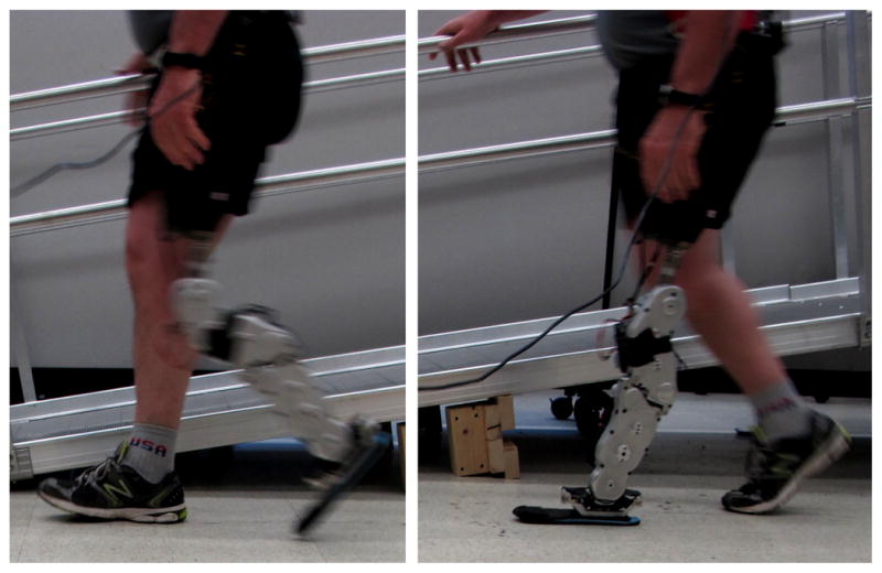
Images of transfemoral amputee subject walking on the Vanderbilt prosthetic leg (designed in [5]) using the proposed virtual constraint strategy.

II. Virtual Constraints for a Prosthetic Leg

We now present a prosthetic control framework that is capable of unifying certain periods of the gait cycle through the use of virtual constraints. After deriving both an exact and an approximate control law for general virtual constraints, we specifically employ the invariance property of effective shape to 1) unify the stance period, 2) coordinate multi-joint control, and 3) enable the prosthesis to accommodate variations in cadence, shoe geometry, and body mass.

A. Modeling the Prosthesis

The prosthetic leg depicted in Fig. 2 (solid gray) is attached to the hip of the body, which is shown in dashed black. We first model the prosthetic leg for our control derivation in this section and return to the full biped model in Section III for the purpose of simulation in Section IV.

Fig. 2.

Kinematic model of transfemoral amputee biped, where the prosthetic stance leg is shown in solid gray and the body in dashed black. The lengths of the heel, shank, and thigh segments are labeled ℓ_f, ℓ_s, and ℓ_t, respectively. The radius of curvature R_f and center of rotation P_f define the rocker foot geometry. Dorsiflexion/plantarflexion of the stance ankle and extension/flexion of the stance knee are defined in the positive/negative directions.

1) Dynamics

We model the prosthetic leg as a kinematic chain with respect to an inertial reference frame attached to the ground (Fig. 2). We define a floating coordinate frame at the prosthetic heel, treating its position coordinates (q_x, q_z) as state variables that will later be constrained by a contact model. The full configuration of the leg in configuration space = ℝ²× is given by q = (q_x, q_z, ϕ, θ_a, θ_k)^T, where ϕ is the foot orientation with respect to vertical, θ_a is the ankle angle, and θ_k is the knee angle. The state of the dynamical system is then given by vector x = (q^T, q̇^T)^T ∈ T , where q̇ ∈ ℝ⁵ contains the joint velocities. The state trajectory evolves according to a differential equation of the form

$$\mathcal{M}(q)\ddot{q}+\mathcal{N}(q,\stackrel{.}{q})+A{(q)}^T\lambda =Bu+J{(q)}^{T}F$$ (1)

where ∈ ℝ^5×5 is the inertia/mass matrix, ∈ ℝ⁵ is a vector that groups the Coriolis/centrifugal terms and gravitational forces, A ∈ ℝ^c×5 is the matrix modeling c physical constraints between the foot and ground, and λ ∈ ℝ^c is the Lagrange multiplier used to calculate the contact forces.

The external forces on the right-hand side of (1) respectively comprise actuator torques and interaction forces with the body. Ankle and knee actuation from torque input u ∈ ℝ² is mapped into the leg’s coordinate system by B = (0_2×3, I_2×2)^T ∈ ℝ^5×2. The interaction force F = (F_x, F_z, M_y)^T ∈ ℝ³ at the socket—the connection between the prosthesis and body at the hip in Fig. 2—comprises two linear forces and a moment in the sagittal plane [25], which can be measured by a 3-axis load cell at the socket. Force vector F acts at the end-point of the leg’s kinematic chain and is mapped to joint torques/forces by the body Jacobian matrix J(q) ∈ ℝ^3×5, which we model using the standard procedure in [26].

2) Stance Period

During the prosthesis stance period we must model the physical forces associated with contact between the prosthetic foot and ground. These contact forces prevent the foot from slipping and falling through the ground, which constitute at least two physical constraints on dynamics (1). Therefore, foot geometry is commonly modeled (e.g., [12]–[15], [27]) as a vector holonomic constraint

$$a(q)=0,$$ (2)

where a: → ℝ^c for c ≥ 2. In Section III we will employ the rocker feet seen in Fig. 2, but other geometries such as flat feet [28], [29] could similarly be modeled in this framework.

Given contact constraint a(q) = 0, we follow the method in [26] to compute the constraint matrix A = ∇_qa and Lagrange multiplier λ = λ̃+λ̃u+λ̄F, where (omitting matrix arguments)

$$\begin{array}{c}\widehat{\lambda }=W(\stackrel{.}{A}\stackrel{.}{q}-A{\mathcal{M}}^{-1}\mathcal{N}),\\ \stackrel{\sim }{\lambda }=WA{\mathcal{M}}^{-1}B,\overline{\lambda }=WA{\mathcal{M}}^{-1}{J}^T\end{array}$$ (3)

for W = (A A^T)⁻¹. These terms enter into dynamics (11) only during the stance period of the prosthetic leg.

3) Swing Period

During the swing period of the prosthesis, the prosthetic foot is not in contact with the ground, so no contact constraints are invoked in the prosthesis dynamics, i.e., λ = 0 in (1). Although the prosthesis is still modeled with respect to its heel point, the interaction force F in prosthesis dynamics (1) suspends the prosthetic leg from the body’s hip.

B. Definition of a Virtual Constraint

Although defined in a similar manner to physical/contact constraints, virtual constraints are enforced by actuator torques rather than external physical forces. The vast majority of virtual constraints used in bipedal robots are holonomic [12]–[16], so we translate these design principles into our prosthetic framework by considering virtual holonomic constraints

$$h(q)=0,$$ (4)

where h: → ℝ² for an actuated knee and ankle, i.e., one virtual constraint per actuated degree-of-freedom (DOF).

Remark 1

Meaningful virtual constraints, i.e., output functions h(q), can be defined in a variety of ways. Reviewing previous work in bipedal robotics (e.g., [12], [13], [15]), virtual constraints can be used to control the actuated joints specified by h₀(q) = (θ_a, θ_k)^T to a desired trajectory h_d(Θ (q)) ∈ as a function of a monotonic quantity Θ(q) ∈ ℝ. This quantity, known as the phase variable or timing variable, provides a unique representation of the gait cycle phase to drive forward the desired pattern in a time-invariant manner. In this case, the output function of equation (4) would be defined by h(q) = h₀(q) − h_d(Θ(q)). The desired pattern h_d can be defined first as a function of time (via boundary-constrained optimization) and then re-parameterized into a function of Θ(q) [12]. We will see that h(q) can also be defined directly from geometric relationships found in human walking, without specifying a desired angular trajectory.

Given desired virtual constraints (4), the goal of a virtual constraint controller is to drive output function h(q) to zero. Therefore, the control system output

$$y:=h(q)$$ (5)

corresponds to tracking error from the desired constraint (4).

Some torque control methods are better suited than others at driving this output to zero. If we do not start with a desired joint pattern h_d (Remark 1), it is not always possible to solve a virtual constraint (4) for a unique joint trajectory as needed for joint impedance methods [4]–[7]. Bipedal robots typically enforce virtual constraints using partial (i.e., input-output) feedback linearization [12], which has appealing theoretical properties including exponential convergence [30], reduced-order stability analysis [12], and robustness to model errors [13]. However, the application of this method to prosthetics presents unique challenges with human-machine interaction.

C. Partial Feedback Linearization of the Prosthesis

We cannot expect to have either a model of the human or sensors at intact joints in a clinically viable system. The controller should then rely only on the prosthesis model, i.e., terms in (1), and feedback available to onboard sensors, i.e., state x = (q^T, q̇^T)^T and interaction force F. The lack of full state feedback from the biped system presents a challenge not previously encountered in implementations of partial feedback linearization on bipedal robots [13]. Therefore, in this section we show that measurements of interaction force F will allow us to achieve similar results on a prosthetic leg.

As previously stated, our goal is to define a feedback control law for input u that drives output y to zero in dynamics (1). An input-output linearizing control law is derived in [19] using Lie derivative notation from [30], but for clarity here we derive an equivalent control law in terms of the matrices in (1). We start by examining the first-order output dynamics ẏ = (∇_qh)q̇. Because the control input u does not appear in these dynamics, output y has relative degree greater than one (cf. [30]) and another time-derivative is needed to expose the control input. Letting H:= ∇_qh, the second-order output dynamics are

$$\begin{array}{l}\ddot{y}=\stackrel{.}{H}\stackrel{.}{q}+H\ddot{q}\\ =\stackrel{.}{H}\stackrel{.}{q}+H{\mathcal{M}}^{-1}(-\mathcal{N}-A^T\lambda +Bu+J^{T}F)\\ =\stackrel{.}{H}\stackrel{.}{q}-H{\mathcal{M}}^{-1}(\mathcal{N}+A^T\widehat{\lambda })+H{\mathcal{M}}^{-1}(B-A^T\stackrel{\sim }{\lambda })u+H{\mathcal{M}}^{-1}(J^T-A^T\overline{\lambda })F.\end{array}$$ (6)

The output function y = h(q) can be chosen such that the 2 × 2 decoupling matrix

$$\begin{array}{l}D(q):=H{\mathcal{M}}^{-1}(B-A^T\stackrel{\sim }{\lambda })\\ =H{\mathcal{M}}^{-1}(I-A^{T}WA{\mathcal{M}}^{-1})B\end{array}$$ (7)

is non-singular over feasible walking configurations, which can be verified numerically. We can then solve for the control law that inverts the output dynamics (6):

$$u_{\text{linz}}:=D^{-1}[-\stackrel{.}{H}\stackrel{.}{q}+H{\mathcal{M}}^{-1}(\mathcal{N}+A^T\widehat{\lambda })-H{\mathcal{M}}^{-1}(J^T-A^T\overline{\lambda })F+u_{\text{pd}}].$$ (8)

Defining a proportional-derivative (PD) input

$$u_{\text{pd}}:=-K_{\mathrm{p}}y-K_{\mathrm{d}}\stackrel{.}{y}$$ (9)

with positive-definite K_p, K_d ∈ ℝ^2×2, control law (8) renders the output dynamics (6) linear and exponentially stable:

$$\ddot{y}=u_{\text{pd}}=-K_{\mathrm{p}}y-K_{\mathrm{d}}\stackrel{.}{y}.$$ (10)

Remark 2

The linear output dynamics (10) imply y(t) → 0 exponentially fast as t → ∞ for y(0) ≠ 0. The feedback linearization provides y ≡ 0 in steady-state, implying that the surface = {x | y = 0, ẏ = 0} is invariant³ under the closed-loop continuous dynamics. This allows system (1) to be restricted to lower-dimensional zero dynamics on surface , where holonomic virtual constraints provide greater dimensionality reduction than nonholonomic constraints [12], [30]. The holonomic outputs characterize the two actuated DOFs, whereas the zero dynamics represent the unactuated DOFs (q_x, q_z, ϕ) coupled with the human through interaction force F. These lower-dimensional dynamics determine the continuous behavior of the full system (1) through the virtual constraints. Classical results in [30] can be invoked to show that the full system is stable if the zero dynamics are stable under control law (8). However, walking has discontinuous impact events (Section III), so surface may not be hybrid invariant, i.e., y = 0 immediately before heel strike may not imply y = 0 immediately after heel strike. We will see in Section IV that the PD terms in (10) quickly correct errors from impacts, by which we approximate hybrid zero dynamics to provide stability of the full hybrid system (cf. [12]). We will exploit the existence of passive gaits down shallow slopes [31] to stabilize the hybrid zero dynamics (and therefore the full hybrid system) in the simulations of Section IV. Similarly, the human wearing the prosthesis will help stabilize the hybrid zero dynamics in the experiments of Section V.

The zero dynamics on are defined by the virtual constraints, independent of the control law enforcing them (and other methods exist, e.g., finite-time control [12], inverse dynamics [29], and control Lyapunov functions [32]). We now present a simpler control law that approximates this partial feedback linearization for our experimental implementation.

D. Approximation of the Partial Feedback Linearization

Although this partial feedback linearization has many beneficial properties, control law (8) can be difficult to implement in practice. Its dependence on interaction force F requires a 3-axis load cell at the socket. This control law also requires an accurate dynamical model (1) of the prosthesis, which could present a barrier to clinical viability when components like prosthetic feet are interchangeable.

We can avoid these potential limitations, while still leveraging the theoretical results of Remark 2, by approximately enforcing virtual constraints with the linear part (9) of control law (8). With sufficiently large PD gains in matrices K_p, K_d, the linear terms will dominate the nonlinear terms in (8). We therefore approximate the exact control law u_linz using only the output PD control law u_pd. Virtual constraints are typically implemented in this approximate manner on experimental bipedal robots [12]–[15].

Remark 3

If the decoupling matrix D(q) is positive-definite and the PD gains are sufficiently large, the outputs will remain close to zero in the output dynamics (6) under control law (9). The prosthesis dynamics (1) will then be close to the zero dynamics in Remark 2, providing a lower-dimensional system for the human-in-the-loop to stabilize. Alternatively, the human interaction force in (6) may help enforce the virtual constraints, allowing the use of small gains in controller (9) as we will see in Section V.

Although control law (9) is linear in the outputs, these outputs are typically nonlinear functions of configuration q, e.g., the phase variable Θ(q). In the next section we will choose these nonlinear functions such that their dependence on a phase variable allows a prosthetic leg to perform phase-specific behaviors that mimic able-bodied human gait.

E. Choosing the Virtual Constraints

The goal of this paper is to implement virtual constraints that unify the stance period, coordinate ankle and knee control, and accommodate clinically meaningful conditions on a powered prosthetic leg. For this purpose we employ a geometric relationship of the stance leg that is invariant across walking conditions including gait speed, shoe geometry, and body weight [21]. This invariance property, known as the effective shape in the prosthetics field, is often used as a metric for aligning passive prostheses [33]. We define the effective shape and show that it can be treated as a virtual holonomic constraint with certain assumptions about the stance contact model—the swing period is considered later.

1) Definition of Effective Shape

Reviewing the preliminary works [19] and [20], an effective shape characterizes how the stance leg joints move as the COP travels from heel to toe. Able-bodied humans have effective shapes specific to activities such as walking [21], stationary swaying [34], and stair climbing [35], and each shape can be characterized by the curvature of the COP trajectory with respect to a reference frame attached to the stance leg. In particular, the ankle-foot (AF) effective shape is the COP trajectory mapped into a shank-based reference frame (axes x̂_s, ẑ_s in Fig. 3, left), and the knee-ankle-foot (KAF) effective shape is the COP trajectory mapped into a thigh-based reference frame (axes x̂_t, ẑ_t in Fig. 3, right). These leg-based frames share an origin at the ankle, but ẑ_s is attached to the knee and ẑ_t to the hip.

Fig. 3.

Diagrams of the ankle-foot (left) and knee-ankle-foot (right) effective shapes. The COP moves along each shape (dashed curve) in the shank-based or thigh-based coordinate frame (solid axes).

These two shapes can be modeled by the distance between the COP and a point P_i = (X_i, Z_i)^T attached to the respective leg-based reference frame:

$$\Vert P_i-\mathit{COP}\Vert =R_i,i\in \{\mathrm{s},\mathrm{t}\},$$ (11)

where the radius of curvature R_i is approximately constant within standing or walking tasks [34]. These two effective shapes provide two virtual constraints to control two joints—the ankle and knee of the prosthesis.

2) Effective Shape as a Virtual Holonomic Constraint

In order to employ these effective shapes in the linearizing control law (8), equation (11) must be expressed as a holonomic constraint in the coordinates of our leg model. This requires the COP to be a function of the configuration q, despite the fact that the COP is usually expressed as a function of forces [36]. We can treat the COP as a position variable if we assume rolling point contact between the foot and ground, which can be achieved with a rocker foot as depicted in Fig. 2. This modeling assumption originates from works showing that rocker feet are suitable substitutes for compliant feet, which are difficult to model, when simulating human-like dynamic walking [27], [37] and when designing prosthetic feet [38]. This contact model is defined in Section III-B and Appendix A, and its limitations are discussed in Section IV-E.

We can now express the vector from the COP to the center of rotation P_i as a function $P_i^{\mathit{COP}}(q)$, i ∈ {s, t}, as defined in Appendix B. Equation (11) is then given in model coordinates by the kinematic constraint h_i(q) = 0 for

$$h_i(q):=R_i-\text{norm}(P_i^{\mathit{COP}}(q)),i\in \{\mathrm{s},\mathrm{t}\}.$$ (12)

This function is the output of a virtual constraint, which corresponds to the distance from the desired effective shape. Hence, the vector output of the AF and KAF virtual constraints is defined as y:= h(x) = (h_s(x), h_t(x))^T.

Remark 4

These effective shapes are virtually enforced on a prosthetic leg by driving output y to zero, which can be achieved exactly using control law (8) or approximately using (9). Virtual constraints (12) depend on the COP, which moves monotonically from heel to toe during steady walking. This choice of constraints should then synchronize the knee and ankle patterns through their mutual dependence on the COP as a phase variable, i.e., Θ(q) = q_x in Remark 1.

Because an effective shape is not defined for the swing leg (which has no COP), we will instead control the swing period with the clinically familiar concept of joint impedance—the stiffness and viscosity of a joint—which is the current standard for controlling powered prosthetic limbs [5]–[7]. We will use joint PD control for this purpose in Sections III–V. Our feedback linearization approach could be used during swing with another choice of virtual constraints, but in this paper we focus on the stance period as a starting point for the first application of this theory to a prosthetic leg.

Now that we have derived an exact and an approximate partial feedback linearization for clinically-motivated virtual constraints, we should validate the feasibility and analyze the robustness of this prosthetic control strategy before experimentally implementing it for amputee subjects. We will perform this analysis in simulation, requiring us to model a biped to interact with the prosthetic limb as would an amputee.

III. Modeling an Amputee Biped for Simulation

In this section we model the amputee biped of Fig. 2 for the purpose of simulating a prosthetic leg under virtual constraint control in Section IV. These simulations require us to consider the coupled dynamics of the body and the prosthesis for a total of 8 DOFs. The extended configuration vector is denoted by q_e = (q^T, θ_h, θ_sa, θ_sk)^T ∈ × , where θ_h is the body’s hip angle, θ_sa is the swing ankle angle, and θ_sk is the swing knee angle. For simplicity we assume symmetry in the full biped (i.e., a bilateral transfemoral amputee with two identical prosthetic legs), where each prosthesis uses the same control strategy. The prosthetic legs do not communicate, so each leg interacts with the model’s hip and opposing leg through interaction forces in (1) as it would with a human body, whether or not the opposing leg is prosthetic.

We model a passive human hip in order to 1) test the inherent stability of the prosthesis controller without active human assistance and 2) avoid the impractical task of modeling a realistic human controller. For this purpose we exploit the existence of passive walking gaits, which arise on declined surfaces when the potential energy converted into kinetic energy during each step replenishes the energy dissipated at impacts [28], [31]. This behavior reflects certain characteristics of human gait, such as ballistic swing motion [39] and energetic efficiency down slopes [40]. We therefore model a downhill slope condition to power the hip in these simulations.

A. Control Strategy

Although the control laws in Section II could employ virtual constraints for both the stance and swing periods, this paper focuses on the use of effective shape as a virtual constraint for its invariance properties during stance. Because no effective shape is known for the swing leg [21], we instead use the standard method of joint PD control (often called impedance control) during swing [5]. This passive method can enable ballistic motion of the swing leg as in human walking [39]. Because the prosthesis does not bear the user’s body weight during the swing period, this model-free method can accurately drive the prosthetic joints to flexion angles needed to achieve toe clearance, which is critical to amputee locomotion.

Although the human hip joint is powered by gravity in our simulation, we add a spring-damper to the joint for consistent step placement. Therefore, the vector of control torques for the entire biped (prostheses and amputee) is given by

$${\tau }_e={(B^T,0_{2\times 3})}^T{u}_{\text{st}}+{(0_{1\times 5},1,0_{1\times 2})}^T{u}_{\mathrm{h}}+{(0_{2\times 6},I_{2\times 2})}^T{u}_{\text{sw}}$$

where u_st = u_linz(x) or u_st = u_pd(x), and the hip input u_h ∈ ℝ and the swing prosthesis inputs in u_sw = (u_sa, u_sk)^T ∈ ℝ² have the form

$$u_i:=-k_{\mathrm{p}i}({\theta }_i-{\theta }_i^{eq})-k_{\mathrm{d}i}{\stackrel{.}{\theta }}_i,$$ (13)

where k_pi, k_di, and ${\theta }_i^{eq}$ respectively correspond to the stiffness, viscosity, and equilibrium angle of joint i ∈ {h, sa, sk}. We saturate the prosthesis torques at 80 N·m to simulate the torque limit of the experimental prosthesis in Section V.

B. Hybrid Dynamics

Bipedal locomotion involves both continuous and discrete dynamics, which constitute a hybrid dynamical system. Here we summarize these hybrid dynamics from [19]. The biped’s continuous dynamics are governed by a differential equation of the form (1). Noting that the derivation for control law (8) in Section II did not depend on a specific choice of foot contact constraints, we must first define a contact model.

To model the biped’s contact constraints in the context of Section II-A2, we choose constant-curvature rocker feet to approximate the deformation of human feet during walking [27], [37]. The associated contact constraints (2) are modeled in Appendix A, where $a_1^{\text{roll}}(q)$ constrains coordinates q_x, q_z to an arc of radius R_f, and $a_2^{\text{roll}}(q)$ constrains ϕ to be perpendicular to the arc. The foot does not extend behind the heel link in Fig. 2, so depending on orientation ϕ the rocker may not be in contact with the ground at heel strike (q_x = q_z = 0). In this case the biped rotates about the heel with constraints defined by $a_1^{\text{heel}}(q):=q_x,a_2^{\text{heel}}(q):=q_z$, which fix the heel position to the ground. These constraints model physical contact, whereas the effective shapes in Section II-E serve as virtual constraints for joint control.

Given this contact model, the constraint terms A and λ in dynamics (1) are computed according to the definitions in Section II-A2. We denote the heel contact matrix as A_heel = ∇_qa^heel or A_eheel = ∇_qe a^heel and the rolling contact matrix as A_roll = ∇_qa^roll or A_eroll = ∇_qe a^roll. The model switches from heel contact to rolling contact when the sole intersects the ground, i.e., when $a_2^{\text{roll}}(q)=0$.

One step period then consists of a sequence of heel contact dynamics, a foot-slap impact event, rolling contact dynamics, and a ground-strike impact event with impact map Δ_e:

$$\begin{array}{lll}\hfill {\mathcal{M}}_{\mathrm{e}}{\ddot{q}}_{\mathrm{e}}+{\mathcal{N}}_{\mathrm{e}}+{A_{\mathrm{e}}}_{\text{heel}}^T{\lambda }_{\mathrm{e}}={\tau }_{\mathrm{e}},& \text{if}\hfill & a_2^{\text{roll}}(q_{\mathrm{e}})\ne 0\hfill \\ \hfill {{\stackrel{.}{q}}_{\mathrm{e}}}^{+}=(1-\mathcal{X}{(A_{\text{eroll}}\mathcal{X})}^{-1}{A}_{\text{eroll}}){{\stackrel{.}{q}}_{\mathrm{e}}}^{-},& \text{if}\hfill & a_2^{\text{roll}}(q_{\mathrm{e}})=0\hfill \\ \hfill {\mathcal{M}}_{\mathrm{e}}{\ddot{q}}_{\mathrm{e}}+{\mathcal{N}}_{\mathrm{e}}+{A_{\mathrm{e}}}_{\text{roll}}^T{\lambda }_{\mathrm{e}}={\tau }_{\mathrm{e}},& \text{if}\hfill & p_{\gamma }^z(q_{\mathrm{e}})\ne 0\hfill \\ \hfill (q_{\mathrm{e}}^{+},{{\stackrel{.}{q}}_{\mathrm{e}}}^{+})={\mathrm{\Delta }}_{\mathrm{e}}(q_{\mathrm{e}}^{-},{{\stackrel{.}{q}}_{\mathrm{e}}}^{-}),& \text{if}\hfill & p_{\gamma }^z(q_{\mathrm{e}})=0\hfill \end{array}$$

which then returns to the beginning of the sequence for the next step [19]. Note that $\mathcal{X}={\mathcal{M}}_{\mathrm{e}}^{-1}{A_{\mathrm{e}}}_{\text{roll}}^T$, superscripts +/− respectively denote post/pre-impact, and $p_{\gamma }^z(q_{\mathrm{e}})\in ℝ$ is the height of the swing foot heel above ground with slope angle γ. Extended terms are defined as in Section II with respect to the extended configuration q_e. After imposing the contact constraints, the full biped model has one degree of underactuation: foot orientation ϕ, which is constrained to a one-to-one relationship with the COP during rolling contact.

C. Stability of Hybrid Limit Cycles

This hybrid dynamical system can be analyzed for stability as in [28]. Letting $x_{\mathrm{e}}={(q_{\mathrm{e}}^T,{{\stackrel{.}{q}}_{\mathrm{e}}}^T)}^T$ be the state vector for the full biped, walking gaits are cyclic and correspond to solution curves x_e(t) of the hybrid system such that x_e(t) = x_e(t + T) for all t ≥ 0 and some minimal T > 0. These solutions define isolated orbits in state space known as hybrid limit cycles, which correspond to equilibria of the Poincaré map P: G → G, where $G=\{x_{\mathrm{e}}\mid p_{\gamma }^z(q_{\mathrm{e}})=0\}$ is the switching surface indicating heel strike. This return map represents a hybrid system as a discrete system between impact events, sending state x_ej ∈ G ahead one step to x_ej+1 = P (x_ej). A periodic solution x_e(t) then has a fixed point $x_{\mathrm{e}}^{\ast }=P(x_{\mathrm{e}}^{\ast })$.

We verify stability about a fixed point $x_{\mathrm{e}}^{\ast }$ by approximating the linearized map ${\nabla }_{x_{\mathrm{e}}}P(x_{\mathrm{e}}^{\ast })$ through a perturbation analysis [28], [31]. The discrete system is locally exponentially stable (LES) if the eigenvalues of ${\nabla }_{x_{\mathrm{e}}}P(x_{\mathrm{e}}^{\ast })$ are strictly within the unit circle, by which we infer that the hybrid limit cycle is LES [28]. We now use this hybrid model to simulate and analyze our prosthesis control strategy, which will later inform the experiments presented in Section V.

IV. Simulation and Robustness Results

In this section we simulate the prosthesis with the amputee model to validate the virtual constraint approach and analyze its robustness to variable walking conditions, approximate feedback linearization, and noisy measurements of the phase variable. To guide the experiments in Section V, we set the model parameters in Table I to average values of adult males [41] with trunk masses grouped at the hip. We characterized foot compliance using the physical foot radius R_f = 0.3ℓ_L for leg length ℓ_L = ℓ_s + ℓ_t as suggested in [37]. The human hip relied on passive dynamics from a decline of γ = 1.72 deg.

TABLE I.

Simulation Parameters

Parameter	Variable	Value
Hip mass	mh	31.73 [kg]
Thigh mass	mt	9.45 [kg]
Thigh moment of inertia	It	0.1995 [kg·m2]
Thigh/shank length	ℓt, ℓs	0.428 [m]
Shank mass	ms	4.05 [kg]
Shank moment of inertia	Is	0.0369 [kg·m2]
Heel height	ℓf	0.07 [m]
Foot mass	mf	1 [kg]
Foot radius	Rf	0.3(ℓs + ℓt) [m]
Slope angle	γ	1.72 [deg]
KAF/AF effective radius	Rt, Rs	0.41(ℓs + ℓt) [m]
KAF/AF center of rotation	Xt, Xs	0 [m]
KAF/AF proportional gain (linz)	Kpt, Kps	2 · mass [N]
KAF/AF derivative gain (linz)	Kdt, Kds	$1.4\sqrt{K_{\text{ps}}}[\mathrm{N}·\mathrm{s}]$
KAF/AF proportional gain (pd)	Kpt, Kps	400 · mass [N]
KAF/AF derivative gain (pd)	Kdt, Kds	$10\sqrt{K_{\text{ps}}}[\mathrm{N}·\mathrm{s}]$
Swing hip equilibrium angle	${\theta }_{\mathrm{h}}^{eq}$	−22.9 [deg]
Swing hip proportional gain	kph	0.106 [N·m/deg]
Swing hip derivative gain	kdh	0.043 [N·m·s/deg]
Swing knee equilibrium angle	${\theta }_{\mathrm{k}}^{eq}$	17.2 [deg]
Swing knee proportional gain	kpk	0.212 [N·m/deg]
Swing knee derivative gain	kdk	0.036 [N·m·s/deg]
Swing ankle equilibrium angle	${\theta }_{\mathrm{a}}^{eq}$	0 [deg]
Swing ankle proportional gain	kpa	2.12 [N·m/deg]
Swing ankle derivative gain	kda	0.270 [N·m·s/deg]

The effective shape parameters defined in Section II-E were chosen according to previous human subject studies [21]. During walking both the AF and KAF effective shapes have a constant radius of curvature (circular arcs in Fig. 3), and these radii are approximately the same: R_t = R_s = 0.41ℓ_L. The centers of rotation are in front of the leg for level-ground walking, but on downhill slopes these shapes are more plantarflexed [21], e.g., X_s = X_t = 0. The constraint defined by (12) is satisfied when the COP passes through the respective leg-based axis, so the ẑ_i-component of P_i is necessarily given by $Z_i=\sqrt{R_i^2-X_i^2}-{\ell }_{\mathrm{f}}$, for i ∈ {s, t}.

Due to these anatomical normalizations of the effective shape parameters [21], only four PD gains needed to be tuned for the entire stance period. We chose K_ps = K_pt = 2 N/kg and $K_{\text{ds}}=K_{\text{dt}}=1.4\sqrt{K_{\text{ps}}}$ to achieve a desired damping ratio in the linearized output dynamics (10), where

$$K_{\mathrm{p}}=\left(\begin{array}{cc}{K}_{\text{ps}}& 0\\ 0& K_{\text{pt}}\end{array}\right),K_{\mathrm{d}}=\left(\begin{array}{cc}{K}_{\text{ds}}& 0\\ 0& K_{\text{dt}}\end{array}\right).$$ (14)

During the prosthesis swing period, the impedance controller (13) facilitated toe clearance by driving the ankle to its neutral position and the knee to a flexion angle. Other impedance parameters in Table I were manually tuned—replacing this method with virtual constraints is left to future work.

A. Ideal Case of Exact Partial Feedback Linearization

We first report the stable walking gaits achieved with the exact control law (8) under ideal conditions. The biped model was simulated in MATLAB as described in [19]. Once the biped converged to a steady-state gait, we numerically verified that the associated fixed point was LES as in Section III-C.

The hybrid limit cycle is shown in Fig. 4. The model maintained heel contact for 274 ms followed by rolling contact for 572 ms (Fig. 5, left), during which the COP moved monotonically from heel to toe as a phase variable. The heel-to-rolling transition caused a discontinuity in the joint velocities, but controller (8) attenuated the outputs during both contact conditions without saturating the joint torques (Fig. 5). Each ground-strike event introduced output error, i.e., the effective shapes were not hybrid invariant (Remark 2), but the outputs remained small and converged to zero within each step period. This result implies that the controller enforced both effective shapes (Fig. 4, right) and created approximate hybrid zero dynamics (Remark 2) that were stabilized by the passive dynamics of the body. A supplemental video of the simulation is available for download.

Fig. 4.

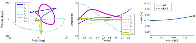
Simulated steady-state gait using the exact control law: angular phase portrait (left), angular trajectories (center), and effective shapes (right). Note that ϕ, θ_a, and θ_k correspond to the stance prosthesis, θ_h corresponds to the body, and θ_sa and θ_sk correspond to the swing prosthesis. The right figure corresponds to the COP trajectory in a shank-based (AF shape) or thigh-based reference frame (KAF shape), where circles indicate contralateral heel strike.

Fig. 5.

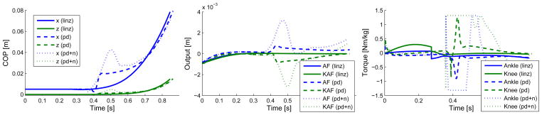
Simulated trajectories of COP (left), outputs (center), and stance leg torques (right) under exact control law (linz), approximate control law (pd), and approximate control law with phase variable noise (pd+n). The foot initially contacts the ground 5 mm in front of the heel to avoid a singularity in the contact model. The outputs correspond to Euclidean distance from the desired effective shape. The torques saturate at ±80 N·m, corresponding to ±1.32 N·m/kg.

B. Robustness to Approximate Partial Feedback Linearization

Although the exact partial feedback linearization produces ideal results, control law (8) can be difficult to implement in practice. We introduced the output PD control law (9) as a clinically viable alternative, which we wish to show approximates the results of the exact control law.

Using the large PD gains in Table I, control law (9) similarly produced a LES walking gait. We see in Fig. 5 (right) that this controller produced larger control torques than did the exact control law, likely because the PD controller used substantially larger gains (but still did not saturate the actuators). These torques dorsiflexed the ankle more and flexed the knee later compared to Fig. 4 (center) from the exact control law. The PD controller allowed output tracking error during mid-stance but corrected most of the error by heel strike (Fig. 5, center), resulting in nearly-constant shape curvature. Although the exact controller performed better, the PD controller reasonably approximated the desired feedback linearization.

We were unable to find stable gaits with PD controller (9) using small gains like those previously used in the exact controller. The exact linearizing controller (8) directly cancels the nonlinear terms in the output dynamics (6), whereas the PD controller (9) must rely on large gains or assistance from the human interaction force to compensate for these nonlinearities (Remark 3). The passive human hip in these simulations cannot actively compensate for instabilities arising from tracking error in the output dynamics, but we will see in the experiments of Section V that human subjects help stabilize the gait when small gains are used. We now show that the approximate feedback linearization retains similar robustness properties to the exact feedback linearization.

C. Robustness to Variable Walking Conditions

Here we report the robustness of both the exact and approximate feedback linearizations across the clinically meaningful conditions of gait speed, ground slope, shoe geometry, and body weight. We separately varied each condition starting from the parameters in Table I, computing the eigenvalues of the steady-state gait across conditions to determine the effect on stability [28], where a maximum absolute eigenvalue (MAE) below one in Fig. 6 implied LES.

Fig. 6.

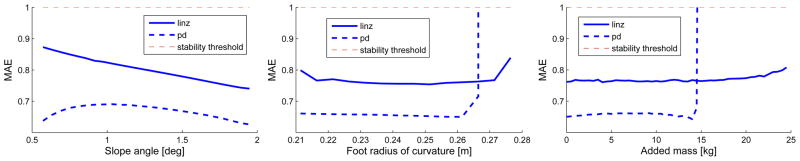
Maximum absolute eigenvalue (MAE) over slope angle (left), foot radius (center), and body weight (right) during steady-state walking with both control laws. A MAE value below one indicates a LES steady-state gait at the x-axis condition.

Because we relied on downhill passive dynamics to model the human part of the biped, we could not directly command the amputee model to walk at different speeds. However, walking speed typically has a one-to-one relationship with ground slope in passive dynamic walking [28], [31], i.e., steeper slopes result in faster speeds. We therefore varied the slope—without changing controller parameters—to examine robustness to variations in both walking speed and terrain. We see in Fig. 7 that gait speed changed linearly with ground slope, where the prosthesis accommodated speeds between 0.68 and 1.06 m/s using both control laws. Despite the use of a passive hip, the amputee model achieved stable walking on slopes very close to level ground (Fig. 6, left), with the closest being a 0.57 deg decline. The biped could not walk stably on level ground without active contribution from the human body, but modeling a hip controller was beyond the scope of this paper. We will instead rely on the amputee experiments of Section V to demonstrate variable cadences on level ground.

Fig. 7.

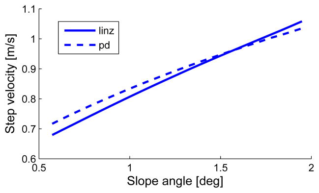
Step velocity over slope for steady-state gait under both control laws.

We studied invariance across shoe geometries by varying the foot radius R_f as suggested by [24]. The stable eigenvalues in Fig. 6 (center) imply some robustness to different foot models, where the exact control law was able to accommodate a slightly greater range than the approximate control law. These simulations suggest that an experimental implementation of the control strategy may be robust to different prosthetic feet or shoes worn by amputees [23], [24].

We increased the human hip mass m_h in Fig. 6 (right) to simulate a subject carrying heavy weights as suggested by [21]. The new weight was unknown to the prosthetic leg except through measurements of the interaction force in the exact control law (8). The prosthesis accommodated up to 24.5 kg in addition to the original body mass (almost a two-fold increase) using the exact control law and up to 14.5 kg using the approximate control law, which has no interaction force measurement. Notably the body weight had little effect on how well the exact control law tracked the outputs (Fig. 8). These simulations demonstrate that both the exact and approximate linearizations can enforce the invariant property of effective shape to accommodate variations in experimental conditions.

Fig. 8.

Output trajectories under extreme weight with the exact control law.

D. Robustness to Phase Variable Noise and Delay

Because our phase variable, the COP, will be calculated from force measurements (Appendix C), this variable will have more noise than feedback from joint encoders in our experiments. We therefore examined the robustness of the PD controller (9) to measurement noise in the phase variable q_x. Based on a signal analysis of our load cells, we added Gaussian white noise with 2 mm root-mean-squared error to simulate the noisy signal. We then applied a fourth-order Butterworth filter (10 Hz low-pass cutoff) to simulate realistic phase-delay from a digital filter. We represented the COP velocity q̇_x with the numerical derivative of this filtered signal.

Using the same PD gains in Table I, the biped walked in a similar manner to the non-noisy PD condition. The noisy COP signal caused larger peak torques (saturating the actuators) during mid-stance, resulting in a brief non-monotonic period of the true COP and greater output tracking error (Fig. 5). The random noise prevented the biped from converging to a period-one hybrid limit cycle, but its ability to take 50+ steps with little deviation suggests the presence of a stable attractor [31]. This simulation demonstrates the robustness of the approximate controller to noise and phase-delay, further motivating our experimental implementation in Section V.

E. Discussion of Model Limitations

These simulations demonstrate the feasibility and robustness of our control approach despite the limitations of the walking model, particularly with regard to the contact assumptions. We assumed point contact during stance in order to model the effective shape as a holonomic virtual constraint (4). Although rolling point contact may not be a realistic assumption for most prosthetic feet (exceptions include the Shape&Roll foot [38] and running ‘blades’ [2]), rocker foot models approximate the compliant motion of the human ankle-foot complex [21], [37]. We saw that our control strategy can accommodate a range of foot curvatures and non-ideal COP behavior, suggesting some robustness to the contact model. Rocker feet are often modeled without ankle joints, but recent work shows that human gait is better predicted by rocker feet with ankles [27], which may allow enforcement of the effective shapes defined from different leg segments [21]. The experiments of Section V will demonstrate that our holonomic treatment of effective shape has no impact on the approximate controller (9).

Although the rolling contact model provided a monotonic COP trajectory in the exact case, the heel-contact condition resulted in a static COP at the start of each step. This fixed contact condition could be avoided in future work by modeling the foot with an arc behind the heel as in [15], [27]. We will see in our experiments that control law (9) produces a strictly monotonic COP trajectory when a human is in the loop, i.e., the COP acts as the phase variable of the virtual constraints.

Other limitations associated with our simplified walking model include the instantaneous double-support phase and downhill slope condition. The assumption of instantaneous impact (common in dynamic walking models [12]–[16], [28], [31]) allows the use of an algebraic impact map instead of differential equations associated with compliant ground contact. We modeled downhill walking to avoid the need for an active controller at the human hip, demonstrating the inherent stability of the prosthesis controller without human help. We now verify these simulation results, while avoiding the model limitations, by performing experiments with amputee subjects.

V. Transfemoral Amputee Experiments

In this section we experimentally test the clinical viability and robustness of our control strategy with transfemoral amputee subjects walking both overground and at variable cadences on a treadmill. Because of experimental time constraints we did not examine variations in foot geometry or body weight other than differences across subjects.

A. Control Implementation

We implemented the approximate controller (9) on the Vanderbilt leg (Fig. 9), a powered knee-ankle prosthesis developed at Vanderbilt University (see [5] for design details). This device had encoders to measure joint angles/velocities and two brushless DC actuators to provide control of the knee and ankle joints. The leg did not have sensors to measure the foot orientation or COP, requiring us to design and integrate the custom instrumented foot in Fig. 10 (see Appendix C). An onboard microcontroller computed⁴ the desired control torques, which were converted into open-loop current inputs to each actuator—these control loops are depicted in Fig. 11.

Fig. 9.

Photo (left) and schematic diagram (right) of Vanderbilt leg attached to custom instrumented foot.

Fig. 10.

Computer-aided design of custom instrumented foot: a load cell adapter mounted onto a prosthetic foot plate as described in Appendix C.

Fig. 11.

Joint-level and motor-level control loops used to experimentally implement virtual constraint control law (9) on the Vanderbilt leg. The joint-level loop computes control law (9) to determine the desired torques, which are produced by the motor-level loop through open-loop current control of the brushless DC motors. Note that the approximate controller (9) does not require measurements of the socket interaction forces as does the exact control law (8).

The integrated leg-and-foot system provided the feedback needed to implement the output PD control law (9) as in Fig. 11. The control gains in Table II were held constant during the stance period. We introduced a new gain K_dts as the bottom-left term of matrix K_d in (14) to facilitate knee flexion as the ankle plantarflexed for forward propulsion during late stance.

TABLE II.

Initial Experimental Parameters

Parameter	Variable	Value
Prosthesis shank length	ℓs	0.406 [m]
Prosthesis heel height	ℓf	0.10 [m]
Prosthesis foot radius	Rf	0.3(ℓs + ℓt) [m]
Slope angle	γ	0 [deg]
KAF/AF effective radius	Rt, Rs	0.158 · height [m]
KAF/AF center of rotation	Xt, Xs	−0.02 · height [m]
KAF proportional gain	Kpt	2 · mass [N]
AF proportional gain	Kps	1 · mass [N]
KAF derivative gain	Kdt	$1.1\sqrt{K_{\text{pt}}}[\mathrm{N}·\mathrm{s}]$
AF derivative gain	Kds	$1.1\sqrt{K_{\text{ps}}}[\mathrm{N}·\mathrm{s}]$
KAF coupled AF-derivative gain	Kdts	−0.5Kdt [N·s]
Swing 1 knee equilibrium angle	${\theta }_{\mathrm{k}}^{eq1}$	80 [deg]
Swing 1 knee proportional gain	kpk1	0.65 [N·m/deg]
Swing 1 knee derivative gain	kdk1	0.04 [N·m·s/deg]
Swing 1 ankle equilibrium angle	${\theta }_{\mathrm{a}}^{eq1}$	0 [deg]
Swing 1 ankle proportional gain	kpa1	2.5 [N·m/deg]
Swing 1 ankle derivative gain	kda1	0.25 [N·m·s/deg]
Swing 2 knee equilibrium angle	${\theta }_{\mathrm{k}}^{eq2}$	0 [deg]
Swing 2 knee proportional gain	kpk2	0.7 [N·m/deg]
Swing 2 knee derivative gain	kdk2	0.08 [N·m·s/deg]
Swing 2 ankle equilibrium angle	${\theta }_{\mathrm{a}}^{eq2}$	0 [deg]
Swing 2 ankle proportional gain	kpa2	2 [N·m/deg]
Swing 2 ankle derivative gain	kda2	0.15 [N·m·s/deg]

The prosthesis employed control law (9) during the stance period, as detected from the vertical force measured by the load cells. When the load dropped below a threshold of about 10% body weight, the prosthesis switched to the impedance-based swing controller (13) from Section III-A. However, the experimental leg had unmodeled joint friction, preventing the ballistic swing motion we observed in our simulations. The knee would not passively extend during late swing as needed to accept the body’s weight in the next step. To compensate for friction and provide clinicians with the ability to prescribe angles for both early knee flexion and late knee extension, we employed two periods of impedance control during swing as commonly done in both passive [3] and powered prostheses [5], [6]. We programmed the control system to switch from one set of impedance parameters (‘Swing 1’ in Table II) to another set (‘Swing 2’ in Table II) when the knee flexion angle reached a threshold of about 70 deg.

For the sake of brevity we defer the details regarding transition rules of the state machine to [6]. We now present the experiments conducted with this prosthetic control system.

B. Experimental Protocol

Three transfemoral amputee subjects were recruited to participate in an experimental study of this prosthetic control system during level-ground walking. All subjects provided written informed consent in accordance with Northwestern University IRB protocol STU00069039. Inclusion criteria required subjects to be aged between 18 to 70 (to reduce the risk of injury), lighter than 113 kg (to meet the load specifications of the prosthesis), and taller than 1.7 m (to allow the subject to walk on the prosthesis without using a lift on the sound foot). Each subject was more than two months post independent ambulation with a unilateral amputation above the knee. During walking trials subjects were provided either a ceiling-mounted harness or handrails to mitigate the risk of injury from falls. A certified prosthetist and an occupational therapist provided clinical support during the experiments and ensured the comfort and safety of the subjects.

At the beginning of each experiment, three anatomical measurements were taken from the subject: body mass [kg], height [m], and residual thigh length ℓ_t [m] between the prosthetic knee joint and the subject’s hip joint. These three measurements alone allowed us to set all the control parameters needed for the subject to begin walking on the prosthesis. We set the shape parameters for level-ground walking using the height-normalized⁵ formulae R_s = R_t = 0.158 · height and X_s = X_t = −0.02 · height based on able-bodied observations in [22]. We then set $Z_{\mathrm{s}}=\sqrt{R_{\mathrm{s}}^2-X_{\mathrm{s}}^2}-{\ell }_{\mathrm{f}}$ and $Z_{\mathrm{t}}=\sqrt{R_{\mathrm{t}}^2-X_{\mathrm{t}}^2}-{\ell }_{\mathrm{f}}$ by definition of effective shape. All subjects started with the same weight-normalized PD gains in Table II for stance control law (9). Even though simulations with this controller in Section IV-B suggested the use of large PD gains, we adopted small gains from the exact controller (8) in Section IV-A to ensure the safety of our subjects. The impedance parameters used for swing control (Table II) were obtained from the impedance-only control strategy in [6].

After loading the subject’s parameters into the prosthetic control system, the subject was instructed to walk back and forth along a short level path between parallel bars (2–3 prosthesis steps per pass). All three subjects were able to walk with the initial set of normalized parameters, but 15 to 45 minutes were dedicated to fine-tuning the parameters (and in some cases the transition rules of the state machine [6]) to maximize the subject’s comfort. For example, TF01 desired more ankle power, so we increased the ankle gain to K_ps = 1.1 · mass. The two other subjects requested slightly less ankle power, for which we lowered the ankle gains. The final gains employed by the three subjects were quite similar, with only minor adjustments made from the initial parameters at the request of the subject or clinical staff.

Once the subjects became comfortable with the prosthetic control system, they were instructed to make 10 consecutive passes along an extended walkway (4–5 prosthesis steps per pass, Fig. 1) without using the parallel bars unless needed for stability. After completing the overground trials, subjects were instructed to walk on a level treadmill at 3 different speeds (within the range simulated in Fig. 7) to test the invariance of the controller. We first allowed the subjects to find a comfortable self-selected speed on the treadmill, which was between 0.8 and 0.9 m/s for all subjects. We recorded 20 prosthesis steps at this ‘normal’ speed. We then increased the speed by 0.134 m/s and recorded 20 prosthesis steps at the resulting ‘fast’ speed. Finally, we decreased the self-selected speed by 0.134 m/s and recorded 20 prosthesis steps at this ‘slow’ speed. No changes to control law (9) were made between speeds. A supplemental video of the treadmill and overground experiments is available for download.

C. Experimental Results

We analyzed the experimental data by first applying a second-order Butterworth filter (12 Hz low-pass cutoff) and segmenting steps based on the vertical load measured by the foot. For overground trials we discarded turn-around steps at the end of each walkway pass as well as the step immediately following this transition. The timeline for each step was normalized between initial heel strike (0% stance) and toe off (100% stance) before averaging across steps.

Focusing on the stance period of the prosthesis—when the virtual constraint controller was employed—Fig. 12 shows the mean data for 20 overground steps by TF02. We see in Fig. 12a that the COP moved monotonically from heel to toe, implying that it served as the phase variable of the virtual constraints as intended. The outputs of the virtual constraints stayed in a small neighborhood about zero (Fig. 12b), demonstrating that the clinically viable controller (9) reasonably approximated the theoretical controller (8) to enforce the virtual constraints. Our choice of effective shape as the virtual constraints resulted in the ankle and knee patterns progressing as a function of the COP as seen in Fig. 13. Note that the joint patterns look different over the phase variable than over time (Fig. 12c–d) because the COP did not increase linearly with respect to time, i.e., the phase domain in which control law (9) operated was a warped representation of the time domain [42].

Fig. 12.

Prosthesis kinematics/kinetics from TF02 overground trial compared with human data (dashed red) from [36]. Mean values of 20 prosthesis steps are shown in solid blue and error bars (±1 standard deviation) are indicated by a shaded region. The COP (a), ankle and knee outputs (b), ankle and knee angles (c–d), estimated ankle and knee torques (e–f), and estimated ankle and knee powers (g–h) are shown over percentage of stance period, i.e., normalized time. Note that the prosthesis torques are estimated from the open-loop motor current (and do not account for extensor moments from the knee hard stop), and these torque estimates are used to approximate the joint powers. All torques and powers are normalized by the total mass of the subject and prosthesis.

Fig. 13.

Prosthetic ankle angle (left) and knee angle (right) as a function of COP during TF02 overground trial. Mean values of 20 prosthesis steps are shown by a solid blue curve, ±1 standard deviation of the COP by horizontal red bars, and ±1 standard deviation of the joint angle by vertical blue bars.

We did not observe any meaningful differences between the overground and treadmill conditions besides reduced variance in the treadmill data. The phase portraits of the three subjects during the treadmill condition (Fig. 14) suggest the existence of a stable limit cycle. As predicted by our simulations, the controller maintained invariant effective shapes across the three treadmill speeds (Fig. 15), resembling able-bodied behavior reported in [22]. The maximum speed reached by the subject pool was 1.03 m/s (TF01), which is notably fast for a transfemoral amputee. We see in Fig. 16 that this subject achieved a natural vertical ground reaction force (GRF) profile with the prosthesis, including an initial hump during early-stance loading and a final hump at late-stance pushoff. This second hump, which is indicative of active propulsion, cannot be achieved with most transfemoral prostheses [2].

Fig. 14.

Prosthetic phase portrait (joint angles vs. velocities) over 20 gait cycles for self-selected treadmill condition of subjects TF01 (left), TF02 (center), and TF03 (right), compared to mean able-bodied (AB) data from [36]. Note that the able-bodied data does not necessarily match each amputee subject’s weight or speed. The prosthetic joint trajectories appear to converge to a periodic orbit—known as a limit cycle—as the subject approached steady state. We suspect that TF03, whose weight was at the upper bound of our inclusion criteria, experienced greater variability because of more frequent actuator saturation.

Fig. 15.

Prosthetic effective shapes at variable cadences from TF01 treadmill trial (averaged across 20 steps for each cadence), compared with able-bodied shapes from overground walking at normal cadence reported in [22]. End of stance is indicated by a circle. The prosthetic effective shapes appear to be invariant across cadences as observed in able-bodied studies [22]. A ‘hook’ occurs during double support in both the prosthetic and able-bodied shapes.

Fig. 16.

Vertical GRF measured from instrumented prosthetic foot during TF01 fast treadmill trial, compared with Winter’s data measured from a force plate during overground walking [36]. The profiles are scaled vertically to compensate for differences in task and measurement technique. Mean values of 20 prosthesis steps are shown in solid blue and error bars (±1 standard deviation) are indicated by a shaded region. Note the double-hump in the force profile—one during early-stance loading and one during late-stance pushoff.

Analysis of the prosthetic joint kinematics and kinetics reveals that the virtual constraint controller produced joint behavior that was close to normal. The ankle angle trajectory in Fig. 12c follows the same trends as Winter’s able-bodied data [36], starting with a period of controlled plantarflexion as the foot progressed from heel-strike to foot-flat. Subsequently as the leg rotated over the foot, the ankle dorsiflexed until a peak of about 13 degrees was reached at about 70% of stance. The movement then reversed as the ankle actively plantarflexed, which we see in the torque estimated from the motor current in Fig. 12e. At this point the controller provided a powered push-off (Fig. 12g), thus contributing actively to the energetics of walking. The ankle did not reach the physiologically appropriate peak torque because its actuator saturated at 80 N · m (see Fig. 12e). Note that the differences between the experimental torques here and the simulated torques in Section IV can be attributed to inaccuracies in the contact model (Section IV-E) and the downhill slope condition used in the simulations, requiring different values for shape parameters X_s, X_t, Z_s, and Z_t in the prosthesis controller.

Although the prosthesis controller provided knee flexion during early stance in the simulations of Section IV, we did not observe this natural behavior in our experiments (Fig. 12d). All subjects intentionally locked the knee while loading body weight on the leg, which most prosthesis users do to ensure the knee does not buckle [2]. The knee torque plot of Fig. 12f does not show a subsequent extensor moment as in Winter’s data, but examination of the prosthetic knee angle shows that the joint was against the hard stop at 4 degrees, which provided an unmeasured extensor moment. Late-stance knee flexion was close to natural and in synergy with ankle push-off, allowing the transfer of positive propulsive energy to the user. In fact, the total mechanical work done by the prosthetic leg during stance (normalized by the mass of the subject and prosthesis) was positive for two of the three subjects: 0.0817 J/kg for TF16, 0.0436 J/kg for TF01, and −0.0541 J/kg for TF02, compared to 0.109 J/kg in Winter’s able-bodied data. We suspect that the prosthesis did negative net work for TF02 because of his use of the handrails (which may have dissipated energy) and less ankle pushoff (at his request).

VI. Discussion

Our control strategy produced close-to-normal walking patterns for transfemoral amputee subjects using normalized effective shape parameters from the literature. The simulations of Section IV verified the robustness of the virtual constraint approach to experimental conditions, and by approximating the desired partial feedback linearization we appeared to achieve stability in our experiments. We observed convergence to a periodic orbit—known as a hybrid limit cycle—in the phase portraits of Fig. 14, suggesting that the controller enabled a steady-state gait pattern for the amputee subjects. Given that the outputs remained in a small neighborhood about zero, control law (9) created approximate hybrid zero dynamics that were stabilized by the human-in-the-loop, demonstrating successful human-machine interaction in the context of virtual constraints. In fact, most subjects did not use the handrails to maintain gait stability with the experimental prosthesis.

A. Strengths of the Approach

This work shows that knee and ankle control during stance can be coordinated by one simple objective: maintaining a constant curvature in the effective shapes. Coordination and synchrony between leg joints (e.g., through biarticular muscles) are important to energetic efficiency [43] and robustness [19], but coordinated control is uncommon in current multi-joint prostheses. Control law (9) coordinated knee control with the ankle joint to enforce the KAF effective shape, which explicitly depends on the ankle angle (Appendix B). Knee and ankle patterns were also synchronized by their dependence on the same phase variable (Remark 4). One subject claimed to notice the two joints working in unison.

By relying on meaningful parameters for clinicians, the proposed control approach could potentially improve the clinical viability of powered prosthetic legs. The effective radii R_s = R_t and centers X_s = X_t are defined by simple fractions of the user’s height [22], preventing the need for hand-tuning. We also demonstrated that the five non-anatomical parameters K_ps, K_pt, K_ds, K_dt, and K_dts can be normalized by body mass as a starting point for walking on the prosthesis. These are the only hand-tuned parameters for stance, whereas existing approaches have more hand-tuned parameters for this period (e.g., 18 for impedance control with three stance phases [5] or more with Hill-type muscle models [7]). By using one control model during stance, we also eliminated two control switches and their hand-tuned rules compared to [5], [7]. However, future randomized clinical studies are needed to compare the performance of these different control methods.

The invariance of the effective shape across conditions such as walking speed [22], heel height [23], shoe curvature [24], and body weight [21] suggests that this choice of virtual constraint could make prosthetic legs more adaptable than conventional prostheses, which cause discomfort and instability as these conditions vary. Our treadmill experiments verified the simulations showing that our control system adjusts to variable walking speeds by enforcing the effective shapes. Although the AF effective shape can also be achieved with the passive Shape&Roll foot [38], this below-knee device cannot regulate the KAF effective shape. Moreover, this passive prosthesis can only be tuned to one task at a time, whereas humans employ effective shapes unique to different tasks. For example, the shape curvature changes substantially between walking and stationary standing [34], and upstairs climbing requires a completely different geometry [35] with positive mechanical work. For this purpose virtual constraints can be defined with non-constant curvature in (12), where the effective shapes associated with stairs may be the most difficult to model [35]. Our control method could implement virtual constraints for any effective shape, by which a powered prosthetic leg could perform a wide variety of tasks.

We did not explicitly design an ankle push-off period into the control strategy, but enforcing the effective shape as a virtual constraint provided a period of power generation as the COP approached the toe. A positive feedback loop arose when COP movement caused a plantarflexive ankle torque, which in turn caused the COP to move further forward. During early stance this positive feedback loop was counteracted by a negative feedback loop involving the moment arm from shear forces. Because forces are transferred down the leg from the socket, subjects were able to influence these feedback loops and consequently their progression through the step. We believe this allowed subjects to walk at their preferred speed overground and accommodate variable speeds on the treadmill. Positive force feedback has been observed during late stance in able-bodied gait [44], but this biomimetic behavior was only previously reproduced in a prosthesis using muscle reflex models [7]. Although we did not tune our control system to maximize positive work, the energy production we observed was likely associated with this positive feedback. This feature in a prosthetic leg might prevent compensatory work at the hip [3] and allow lower-limb amputees to expend normal levels of energy when walking [2]. However, this positive feedback loop should be disabled during stationary standing, as COP drift towards the toe could cause unintended ankle pushoff.

B. Limitations of the Study

The use of approximate feedback linearization resulted in a few discrepancies during mid-late stance. Excessive ankle dorsiflexion in Fig. 12c was associated with tracking error from the desired effective shapes, which grew during mid-late stance in both the simulations (Fig. 5) and experiments (Fig. 12b). We suspect that the approximate controller could not compensate for stronger nonlinearities during this period of gait, especially in the presence of ankle actuator saturation (Fig. 12e) and small PD gains. We employed small gains for the safety of our subjects, who may have helped virtual constraint enforcement through the socket interaction forces, which enter into the output dynamics (6). Future work could compensate for nonlinearities by using larger PD gains during mid-late stance (via phase-based gain scheduling), simultaneous linear control methods [45], or the exact feedback linearization of Section II-C. Performance could be further improved with series elastic actuation [46], which can provide closed-loop torque control and larger peak torques.

The prosthetic foot used in these experiments violated our model’s point-contact assumption (the COP was not dependent on configuration alone as assumed in Section II-E), implying that the effective shape was not truly holonomic. Our experiments successfully employed these nonholonomic constraints, e.g., output functions of the form h(q, q̇), in the approximate control law (9), demonstrating some robustness to unmodeled dynamics. The exact control law (8) could also be reformulated for nonholonomic constraints as in [29], resulting in lower-order output dynamics and higher-order zero dynamics. However, the vast majority of bipedal robots [12]–[16] use holonomic virtual constraints for lower-dimensional stability analysis (Remark 2), motivating our holonomic treatment in this paper. We employed the effective shape as a starting point for this research, but future work could find better choices of virtual constraints for use in the general control framework of Section II.

For example, we could model non-constant curvature into the effective shape during the double-support period to better mimic able-bodied gait (Fig. 15, [21]). For simplicity we continued using the constant-curvature virtual constraints (12) as the prosthesis entered double support with the intact leg. We see in Fig. 15 that the approximate controller (9) provided compliance during this period to resemble able-bodied effective shapes, but the stance-to-swing transition (when the most KAF tracking error occurred) was a source of criticism from the subjects. A more general model of effective shape with non-constant curvature in (11) could potentially be used in the future to explicitly enforce the appropriate shape during double support. Replacing the joint impedance controller of the swing period with a minimum-jerk control strategy [47] may also help the stance-to-swing transition. Alternatively, a definition of effective shape for the swing period would allow the use of virtual constraints, resulting in a unified swing period to further reduce the number of control switches and hand-tuned parameters. This development may require a new phase variable that is measurable from the prosthesis during swing (see initial work in [48]). Only after these promising directions are investigated will the virtual constraint approach be mature enough for clinical comparison with state-of-the-art impedance control methods [4]–[6].

VII. Conclusion

These simulations and experiments demonstrate that the theory of virtual constraints could provide a clinically viable solution for unified control of powered prosthetic legs. In particular, our stance control strategy produced biomimetic, robust, and coordinated ankle-knee movement on a prosthetic leg used by amputee subjects. The controller was able to operate at variable cadences without changes to control parameters due to the invariance of the effective shape, which also holds over shoe geometries and body weights [21].

Our simulations suggest that the proposed control approach can also accommodate inclines, motivating future experiments with ramps and stairs. More demanding tasks like running may require the exact feedback linearization in Section II-C to prevent output tracking error, necessitating system identification of the intrinsic dynamics of the prosthetic leg. Our control approach could also be integrated with a neural interface (e.g., using electromyography from residual muscles [49]) to allow the user to subconsciously switch between virtual constraints when anticipating a task change.

The significance of effective shape begs the question as to whether human locomotion might employ a phase variable [42], [48]. Phase-based virtual constraints could also be applied to powered exoskeletons (e.g., [11]), motivating future investigation of hybrid zero dynamics for wearable robots. With further development the proposed control concepts have the potential to improve mobility and quality of life for individuals after amputation, stroke, or spinal cord injury.

Biographies

Robert D. Gregg (S’08-M’10) received the B.S. degree (2006) in electrical engineering and computer sciences from the University of California, Berkeley and the M.S. (2007) and Ph.D. (2010) degrees in electrical and computer engineering from the University of Illinois at Urbana-Champaign.

He joined the Departments of Bioengineering and Mechanical Engineering at the University of Texas at Dallas (UTD) as an Assistant Professor in 2013. Prior to joining UTD, he was a Research Scientist at the Rehabilitation Institute of Chicago and a Postdoctoral Fellow at Northwestern University. His research is in the control of bipedal locomotion with applications to autonomous and wearable robots.

Prof. Gregg is a recipient of the NIH Director’s New Innovator Award and the Burroughs Wellcome Fund’s Career Award at the Scientific Interface. He also received the 2011 CLAWAR Best Technical Paper Award, the 2009 O. Hugo Schuck Award of the IFAC American Automatic Control Council, and the Best Student Paper Award of the 2008 American Control Conference.

Tommaso Lenzi (S’11-M’13) received the M.Sc. degree in biomedical engineering from the University of Pisa, Pisa, Italy, in 2008, and the Ph.D. degree in biorobotics, from Scuola Superiore Sant’Anna, Pisa, Italy, in 2012. He is currently a Postdoctoral Fellow with the Center for Bionic Medicine, Rehabilitation Institute of Chicago, and the Department of Physical Medicine and Rehabilitation, Northwestern University, Chicago, IL, USA. From August 2011 to February 2012, he was Visiting Research Scientist with the Department of Mechanical Engineering, University of Delaware, Newark, DE, USA. He has co-authored 16 ISI journal papers and 29 peer-review conference proceedings papers. His main research interests include robotics, mechatronics, and rehabilitation medicine, with a major emphasis on design and control of wearable robots for human assistance and rehabilitation.

Levi J. Hargrove (S’05-M’08) received his B.Sc. and M.Sc. and PhD degrees in electrical engineering from the University of New Brunswick (UNB), Fredericton, NB, Canada, in 2003 2005, and 2007 respectively. He joined the Center for Bionic Medicine at the Rehabilitation Institute of Chicago in 2008. His research interests include pattern recognition, biological signal processing, and myoelectric control of powered prostheses. Dr. Hargrove is a member of the Association of Professional Engineers and Geoscientists of New Brunswick. He is also an Assistant Professor in the Department of Physical Medicine and Rehabilitation (PM&R) and Biomedical Engineering, Northwestern University, Evanston, IL, USA.

Jonathon W. Sensinger (M’09) received the B.S. degree in bioengineering from the University of Illinois, Chicago, IL, USA, in 2002, and the Ph.D. degree in biomedical engineering from Northwestern University, Chicago, IL, USA, in 2007.

He is currently the Associate Director of the Institute of Biomedical Engineering and an Associate Professor of Electrical and Computer Engineering at the University of New Brunswick, Fredericton, NB, Canada. His research interests include body-powered and robotic prosthesis design and control, with interest in developing-world applications. He focuses on clinically relevant, low cost/weight systems. In addition, he performs research in human-machine interfaces using haptics and computational motor control approaches with a goal to improve the control filtering and sensory feedback options available to persons with an amputation.

Appendix

A. Contact Constraints

Because a rolling contact point has zero velocity at any instant [25], we simplify model-based calculations by treating this contact point (the COP) as stationary and modeling the kinematic chain with respect to an inertial frame defined at the COP. This assumption physically corresponds to rolling on an ideal treadmill, which can approximate the curvature of human foot compliance, i.e., the relative motion between the COP and heel, in a similar manner to rolling overground. We model the foot as an arc of radius R_f going through the heel (q_x, q_z) and the COP. The vector from the COP to the center of rotation P_f is defined normal to the ground and constrained by ||P_f –COP || = R_f, yielding equation $a_1^{\text{roll}}(q)=0$. We also constrain the foot orientation ϕ so the heel is perpendicular to the foot arc (Fig. 2), yielding equation $a_2^{\text{roll}}(q)=0$.

B. Virtual Constraints

The AF effective shape is the distance constraint (11) between the COP and the center of rotation P_s in the shank-based reference frame of Fig. 3 (left). In model coordinates q defined with respect to the COP, P_s is given by the function

$$P_{\mathrm{s}}^{\mathit{COP}}(q)={(q_x,q_z)}^T+{\ell }_{\mathrm{f}}{(-sin(\varphi ),cos(\varphi ))}^T+S(\varphi +{\theta }_{\mathrm{a}})P_{\mathrm{s}},$$

where S is the standard 2×2 rotation matrix parameterized by angle ϕ+θ_a. Similarly, the KAF effective shape is the distance constraint (11) between the COP and the center of rotation P_t in a thigh-based reference frame (Fig. 3, right). The point P_t is given in model coordinates by the function

$$P_{\mathrm{t}}^{\mathit{COP}}(q)={(q_x,q_z)}^T+{\ell }_{\mathrm{f}}{(-sin(\varphi ),cos(\varphi ))}^T+S(\rho )P_{\mathrm{t}},$$

where rotation matrix S is parameterized by angle

$$\rho =\varphi +arctan(\frac{{\ell }_{\mathrm{s}}sin({\theta }_{\mathrm{a}})+{\ell }_{\mathrm{t}}sin({\theta }_{\mathrm{a}}+{\theta }_{\mathrm{k}})}{{\ell }_{\mathrm{s}}cos({\theta }_{\mathrm{a}})+{\ell }_{\mathrm{t}}cos({\theta }_{\mathrm{a}}+{\theta }_{\mathrm{k}})}).$$

Finally, these functions define the virtual constraints by (12).

C. Instrumented Foot

We designed the instrumented prosthetic foot in Fig. 10 to measure the COP for our controller as initially reported in [20]. Two aluminum plates were mounted around two 6-axis load cells (model: Mini45, ATI Industrial Automation, Apex, NC) with one cell towards the heel and the other towards the toe. This configuration distributed loads encountered during walking to prevent sensor saturation and bending moments. The top plate was mounted to the bottom of the leg’s ankle joint, and the bottom plate was mounted to a carbon fiber prosthetic foot plate; the configured leg is shown in Fig. 9 (left). The assembled foot adapter (load cells and aluminum plates) added 0.79 kg to the weight of the foot plate.

The two aluminum plates of the foot adapter were mechanically coupled only through the load cells, by which we measured the loads transferred between the leg and ground. We used a free-body diagram to solve for the COP:

$$q_x=\frac{M_{y1}+M_{y2}+b_{\mathrm{v}}(F_{x1}+F_{x2})+b_{\mathrm{h}}(F_{z2}-F_{z1})}{F_{z1}+F_{z2}},$$

where F_xi and F_zi are the horizontal and vertical loads, respectively, at the heel (i = 1) or toe (i = 2), b_v = 5.08 cm is the vertical distance between the bottom of the foot plate and the reference frame of each load cell, and b_h = 7 cm is the horizontal distance between the ankle joint and the reference frame of each load cell (Fig. 10). This calculation requires only three of the six strain gauges in each ATI load cell, which was chosen for compactness, weight, and load ratings. All six strain gauges could be used to measure the 3D GRF vector, allowing selective saturation of control torques to keep the GRF within the friction cone and thus prevent the foot from slipping.

We did not have an inertial measurement unit to measure heel rise and foot rotation, so we approximated these variables based on the rocker-foot contact model in Appendix A.

References

- 1.Miller W, Deathe A, Speechley M, Koval J. The influence of falling, fear of falling, and balance confidence on prosthetic mobility and social activity among individuals with a lower extremity amputation. Arch Phys Med Rehab. 2001;82(9):1238–1244. doi: 10.1053/apmr.2001.25079. [DOI] [PubMed] [Google Scholar]
- 2.Smith DG, Michael JW, Bowker JH, editors. Atlas of Amputations and Limb Deficiencies: Surgical, Prosthetic, and Rehabilitation Principles. Rosemont, IL: American Academy of Orthopaedic Surgeons; 2004. [Google Scholar]
- 3.Johansson J, Sherrill D, Riley P, Bonato P, Herr H. A clinical comparison of variable-damping and mechanically passive prosthetic knee devices. Amer J Phys Med Rehab. 2005;84(8):563–575. doi: 10.1097/01.phm.0000174665.74933.0b. [DOI] [PubMed] [Google Scholar]
- 4.Sup F, Bohara A, Goldfarb M. Design and control of a powered transfemoral prosthesis. Int J Robot Res. 2008;27(2):263–273. doi: 10.1177/0278364907084588. [DOI] [PMC free article] [PubMed] [Google Scholar]
- 5.Sup F, Varol H, Goldfarb M. Upslope walking with a powered knee and ankle prosthesis: Initial results with an amputee subject. IEEE Trans Neural Sys Rehab Eng. 2011;19(1):71–78. doi: 10.1109/TNSRE.2010.2087360. [DOI] [PubMed] [Google Scholar]
- 6.Simon A, Fey N, Finucane S, Lipschutz R, Hargrove L. Strategies to reduce the configuration time for a powered knee and ankle prosthesis across multiple ambulation modes. IEEE Int. Conf. Rehab. Robot; Seattle, WA. 2013. [DOI] [PubMed] [Google Scholar]
- 7.Eilenberg M, Geyer H, Herr H. Control of a powered ankle–foot prosthesis based on a neuromuscular model. IEEE Trans Neural Sys Rehab Eng. 2010;18(2):164–173. doi: 10.1109/TNSRE.2009.2039620. [DOI] [PubMed] [Google Scholar]
- 8.Stein JL, Flowers WC. Stance phase control of above-knee prostheses: Knee control versus SACH foot design. J Biomech. 1987;20(1):19–28. doi: 10.1016/0021-9290(87)90263-6. [DOI] [PubMed] [Google Scholar]
- 9.Holgate MA, Sugar TG, Bohler AW. A novel control algorithm for wearable robotics using phase plane invariants. IEEE Int. Conf. Robot. Automat; Kobe, Japan. 2009. pp. 3845–3850. [Google Scholar]
- 10.Boehler AW, Hollander KW, Sugar TG, Shin D. Design, implementation and test results of a robust control method for a powered ankle foot orthosis (AFO). IEEE Int. Conf. Robot. Automat; Pasadena, CA. 2008. pp. 2025–2030. [Google Scholar]
- 11.Shorter KA, Hsiao-Wecksler ET, Kogler GF, Loth E, Durfee WK. A portable powered ankle-foot-orthosis for rehabilitation. J Rehab Res Dev. 2011;48(4):459–472. doi: 10.1682/jrrd.2010.04.0054. [DOI] [PubMed] [Google Scholar]
- 12.Westervelt ER, Grizzle JW, Chevallereau C, Choi JH, Morris B. Feedback Control of Dynamic Bipedal Robot Locomotion. New York, NY: CRC Press; 2007. [Google Scholar]
- 13.Sreenath K, Park HW, Poulakakis I, Grizzle JW. A compliant hybrid zero dynamics controller for stable, efficient and fast bipedal walking on MABEL. Int J Robot Res. 2011;30(9):1170–1193. [Google Scholar]
- 14.Kolathaya S, Ames AD. Achieving bipedal locomotion on rough terrain through human-inspired control. IEEE Int. Sym. Safety Security Rescue Robot; College Station, TX. 2012. [Google Scholar]
- 15.Martin A, Post D, Schmiedeler J. Design and experimental implementation of a hybrid zero dynamics controller for planar bipeds with curved feet. Int J Robot Res. 2014;33(7):988–1005. [Google Scholar]
- 16.Ramezani A, Hurst JW, Hamed KA, Grizzle JW. Performance analysis and feedback control of ATRIAS, a 3D bipedal robot. ASME J Dyn Sys Meas Control. 2013;136(2):021012. [Google Scholar]
- 17.Espiau B. Sensor-based estimation of human motion for control synchronization. IEEE RO-MAN; Toyama, Japan. 2009. [Google Scholar]
- 18.Gregg RD, Sensinger JW. Towards biomimetic virtual constraint control of a powered prosthetic leg. IEEE Trans Control Sys Tech. 2014;22(1):246–254. doi: 10.1109/TCST.2012.2236840. [DOI] [PMC free article] [PubMed] [Google Scholar]
- 19.Gregg RD, Sensinger JW. Biomimetic virtual constraint control of a transfemoral powered prosthetic leg. Amer. Control Conf; Washington, DC. 2013. pp. 5702–5708. [Google Scholar]
- 20.Gregg RD, Lenzi T, Fey NP, Hargrove LJ, Sensinger JW. Experimental effective shape control of a powered transfemoral prosthesis. IEEE Int. Conf. Rehab. Robot; Seattle, WA. 2013. [DOI] [PubMed] [Google Scholar]
- 21.Hansen A, Childress D. Investigations of roll-over shape: Implications for design, alignment, and evaluation of ankle-foot prostheses and orthoses. Dis Rehab. 2010;32(26):2201–2209. doi: 10.3109/09638288.2010.502586. [DOI] [PubMed] [Google Scholar]
- 22.Hansen A, Childress D, Knox E. Roll-over shapes of human locomotor systems: Effects of walking speed. Clin Biomech. 2004;19(4):407–414. doi: 10.1016/j.clinbiomech.2003.12.001. [DOI] [PubMed] [Google Scholar]
- 23.Hansen A, Childress D. Effects of shoe heel height on biologic rollover characteristics during walking. J Rehab Res Dev. 2004;41(4):547–554. doi: 10.1682/jrrd.2003.06.0098. [DOI] [PubMed] [Google Scholar]
- 24.Wang C, Hansen A. Response of able-bodied persons to changes in shoe rocker radius during walking: Changes in ankle kinematics to maintain a consistent roll-over shape. J Biomech. 2010;43(12):2288–2293. doi: 10.1016/j.jbiomech.2010.04.036. [DOI] [PMC free article] [PubMed] [Google Scholar]
- 25.Hibbeler RC. Engineering Mechanics: Dynamics. 13. Upper Saddle River, NJ: Prentice Hall; 2012. [Google Scholar]
- 26.Murray RM, Li Z, Sastry SS. A Mathematical Introduction to Robotic Manipulation. Boca Raton, FL: CRC Press; 1994. [Google Scholar]
- 27.Martin A, Schmiedeler J. Predicting human walking gaits with a simple planar model. J Biomech. 2014;47(6):1416–1421. doi: 10.1016/j.jbiomech.2014.01.035. [DOI] [PubMed] [Google Scholar]
- 28.Gregg RD, Dhaher YY, Degani A, Lynch KM. On the mechanics of functional asymmetry in bipedal walking. IEEE Trans Biomed Eng. 2012;59(5):1310–1318. doi: 10.1109/TBME.2012.2186808. [DOI] [PMC free article] [PubMed] [Google Scholar]
- 29.Gregg RD, Righetti L. Controlled reduction with unactuated cyclic variables: Application to 3D bipedal walking with passive yaw rotation. IEEE Trans Automat Contr. 2013;58(10):2679–2685. doi: 10.1109/TAC.2013.2256011. [DOI] [PMC free article] [PubMed] [Google Scholar]
- 30.Isidori A. Nonlinear Control Systems: An Introduction. 3. Berlin, Germany: Springer-Verlag; 1995. [Google Scholar]
- 31.Goswami A, Thuilot B, Espiau B. A study of the passive gait of a compass-like biped robot: Symmetry and chaos. Int J Robot Res. 1998;17(12):1282–1301. [Google Scholar]
- 32.Ames AD, Galloway K, Grizzle JW, Sreenath K. Rapidly exponentially stabilizing control Lyapunov functions and hybrid zero dynamics. IEEE Trans Automat Contr. 2014;59(4):876–891. [Google Scholar]
- 33.Hansen A, Childress D, Knox E. Prosthetic foot roll-over shapes with implications for alignment of trans-tibial prostheses. Prosth Orth Int. 2000;24(3):205–215. doi: 10.1080/03093640008726549. [DOI] [PubMed] [Google Scholar]
- 34.Hansen A, Wang C. Effective rocker shapes used by able-bodied persons for walking and fore-aft swaying: Implications for design of ankle-foot prostheses. Gait Pos. 2010;32(2):181–184. doi: 10.1016/j.gaitpost.2010.04.014. [DOI] [PMC free article] [PubMed] [Google Scholar]
- 35.Sinitski E, Hansen A, Wilken J. Biomechanics of the ankle-foot system during stair ambulation: Implications for design of advanced ankle-foot prostheses. J Biomech. 2012;45(3):588–594. doi: 10.1016/j.jbiomech.2011.11.007. [DOI] [PubMed] [Google Scholar]
- 36.Winter DA. Biomechanics and Motor Control of Human Movement. 2. New York, NY: Wiley; 2009. [Google Scholar]
- 37.Adamczyk P, Collins S, Kuo A. The advantages of a rolling foot in human walking. J Exp Bio. 2006;209(20):3953. doi: 10.1242/jeb.02455. [DOI] [PubMed] [Google Scholar]
- 38.Sam M, Childress D, Hansen A, Meier M, Lambla S, Grahn E, Rolock J. The ‘Shape&Roll’ prosthetic foot: I. Design and development of appropriate technology for low-income countries. Med Confl Surviv. 2004;20(4):294–306. doi: 10.1080/1362369042000285937. [DOI] [PubMed] [Google Scholar]
- 39.Mochon S, McMahon TA. Ballistic walking. J Biomech. 1980;13(1):49–57. doi: 10.1016/0021-9290(80)90007-x. [DOI] [PubMed] [Google Scholar]
- 40.Minetti A, Moia C, Roi G, Susta D, Ferretti G. Energy cost of walking and running at extreme uphill and downhill slopes. J Applied Phys. 2002;93(3):1039–1046. doi: 10.1152/japplphysiol.01177.2001. [DOI] [PubMed] [Google Scholar]
- 41.De Leva P. Adjustments to Zatsiorsky-Seluyanov’s segment inertia parameters. J Biomech. 1996;29(9):1223–1230. doi: 10.1016/0021-9290(95)00178-6. [DOI] [PubMed] [Google Scholar]
- 42.Gregg RD, Rouse EJ, Hargrove LJ, Sensinger JW. Evidence for a time-invariant phase variable in human ankle control. PLoS ONE. 2014;9(2):e89163. doi: 10.1371/journal.pone.0089163. [DOI] [PMC free article] [PubMed] [Google Scholar]
- 43.Pedotti A. A study of motor coordination and neuromuscular activities in human locomotion. Bio Cybernetics. 1977;26(1):53–62. doi: 10.1007/BF00363992. [DOI] [PubMed] [Google Scholar]
- 44.Dietz V, Duysens J. Significance of load receptor input during locomotion: A review. Gait Pos. 2000;11(2):102–110. doi: 10.1016/s0966-6362(99)00052-1. [DOI] [PubMed] [Google Scholar]
- 45.Nanjangud A, Gregg RD. Simultaneous control of an ankle-foot prosthesis model using a virtual constraint. ASME Dynamic Systems Control Conf; San Antonio, TX. 2014. [DOI] [PMC free article] [PubMed] [Google Scholar]
- 46.Paine N, Oh S, Sentis L. Design and control considerations for high-performance series elastic actuators. IEEE/ASME Trans Mechatron. 2014;19(3):1080–1091. [Google Scholar]
- 47.Lenzi T, Hargrove LJ, Sensinger JW. A novel control framework allowing physiological walking speed adaptation in powered transfemoral prostheses. IEEE Robot Automat Mag. 2014 in press. [Google Scholar]
- 48.Villarreal DJ, Gregg RD. A survey of phase variable candidates of human locomotion. IEEE Int. Conf. Eng. Med. Biol. Soc; Chicago, IL. 2014. [DOI] [PMC free article] [PubMed] [Google Scholar]
- 49.Hargrove L, Simon A, Lipschutz R, Finucane S, Kuiken T. Real-time myoelectric control of knee and ankle motions for transfemoral amputees. J Amer Med Assoc. 2011;305(15):1542–1544. doi: 10.1001/jama.2011.465. [DOI] [PubMed] [Google Scholar]
Associated Data
This section collects any data citations, data availability statements, or supplementary materials included in this article.