Toward Volumetric MR Thermometry with the MASTER Sequence

Abstract

MR temperature monitoring is an indispensable tool for high intensity focused ultrasound. In this paper, a new technique known as MASTER (Multiple Adjacent Slice Thermometry with Excitation Refocusing) is presented which improves the speed and accuracy of multiple-slice MR thermometry. Defocusing the magnetization after exciting a slice allows for multiple slices to be excited concurrently and stored in k-space. The magnetization from each excitation is then refocused and read in sequence. This approach increases TE for each slice, greatly improving temperature SNR as compared to conventional slice interleaving. Gradient sequence design optimization is required to minimize diffusion losses while maintaining high sequence efficiency. Flexibility in selecting position, update rate, accuracy, and voxel size for each slice independently allows for freedom in design to fit different application needs. Results are shown in phantom and in vivo validating the feasibility of the sequence, and comparing it to interleaved GRE. Sample design curves are presented that contrast the MASTER design space with that of interleaved GRE thermometry.

I. Introduction

High intensity focused ultrasound (HIFU) has been used to perform non-invasive surgical ablation of tumors, fibroids, and other tissues. In MRI-guided Focused Ultrasound (MRgFUS) interventions, MRI is used to guide, monitor, and assess treatments. Transcranial MRgFUS has been used in the brain to treat neuropathic pain [1], [2], brain tumors [3], and essential tremor [4]. During these treatments, MR thermometry is used to verify the position of the focus before treatment and to monitor heating during treatment. Healthy tissue is monitored to ensure that no undesired damage results. Published treatments have used single-slice thermometry sequences for monitoring, but the development of fast multi-slice thermometry would improve monitoring of these treatments. In particular, faster imaging for focal spot verification would decrease treatment time and improve patient comfort. Additionally, greater volumetric temperature monitoring coverage would decrease the possibility of undetected heating in healthy tissue thereby improving patient safety.

A. Thermometry Requirements

During high power sonications, fast and precise temperature mapping is required to accurately calculate the thermal dose being delivered. Individual sonications can be as short as 10 seconds [2], so it is important that any thermometry approach be fast enough to obtain multiple measurements in that time frame for sufficient temporal sampling of the temperature progression. Additionally, the MRI resolution must be on the order of the focal spot size or smaller in order to make accurate measurements. The ExAblate Neuro (Insightec, Haifa, Israel) is able to generate ellipsoidal lesions that are approximately 3-4 mm in diameter and 4-5 mm tall [2]. For temperature monitoring, a resolution of 1-2 mm in-plane and a slice thickness of 3 mm or thinner is desired to achieve accurate temperature measurements [5].

Excessive heating outside of the intended treatment region can be caused by skull absorption [6], uncorrected aberration [7], ultrasound sidelobes [8], or by calcifications in the brain [9]. If undesired heating occurs in the imaging plane, it can be measured with the thermometry sequence prescribed for treatment. However, if undesired heating occurs anywhere else in the brain, it will be undetected by single plane thermometry. Multiple slice thermometry would help in detecting undesired heating and reduce risk of adverse events.

B. PRF Shift Thermometry Measurement Accuracy

MR thermometry predominately uses proton resonance frequency (PRF) shift thermometry [10]–[14], due to its fast and accurate measurement capability in aqueous tissue. The precession frequency of water changes linearly with temperature [15] across all aqueous tissue types, resulting in measured phase changes during gradient echo imaging Because PRF shift thermometry uses phase information, the measurement accuracy (SNR) as a function of TE is different than that of conventional magnitude imaging. Assuming there is no steady state signal, SNR_temperature ∝ TE·e^-TE/T2* [13], [16]. Steady state signal components can alter this SNR relationship [17], though RF spoiling can be used to suppress steady state contributions. In either case, significant SNR improvements are obtained by increasing from a short TE (used in conventional interleaved multi-slice) to a TE close to T2*. Echo shifting [18] and non-Cartesian trajectories [11], [13], [19] have been demonstrated in past work to obtain GRE temperature measurements with longer TEs, shorter acquisition times, or increased volume coverage [20]–[23]. Steady state sequences have also been proposed as an alternative to gradient-echo thermometry [24]. The goal of this work was to design, implement, and test a flexible, new volumetric sequence that uses longer TEs for improved gradient-echo multi-slice thermometry and is compatible with Cartesian and non-Cartesian readouts.

II. Theory

In this study, we present a novel sequence, MASTER, (Multiple Adjacent Slice Thermometry with Excitation Refocusing) for multiple slice MR thermometry with high measurement accuracy, resolution, and speed. For a given update rate (e.g. 5 seconds per frame), the maximum TE of conventional multi-slice interleaved GRE decreases significantly as more slices are collected, reducing temperature measurement accuracy. For an update rate of 5 seconds, a 6 slice sequence (128 phase encodes, 1.5 ms total for excitation and gradient spoiling) has a maximum TE < 5.0 ms, far below the optimal TE for brain tissue of TE = T2* ≈ 50 ms. Multi-line or single shot EPI approaches have been used to accelerate multi-slice thermometry [21]. However, EPI techniques can suffer from distortion artifacts and measurement error [25].

To improve multiple slice temperature measurement accuracy for the time constraint imposed by short sonication durations, the MASTER sequence re-orders the acquisition such that all slices are excited, phase encoding occurs, and then all slices are read out using the full duration of the TR. This is different than conventional multi-slice acquisitions, in which excitation and readout for each slice occurs sequentially, using the duration of the TR divided by the number of slices to acquire each slice. A simplified diagram of the MASTER sequence is shown in Fig. 1, with a multi-slice interleaved GRE sequence diagram shown for comparison. The two sequences have excitations (RF) for each slice, phase encoding, and sampling read outs for each slice. The MASTER sequence adds multiple sections of gradient spoiling and un-spoiling (described later as “excitation defocusing” and “excitation refocusing”). These diagrams show that the TE for MASTER is a much greater fraction of the TR than it is for a comparable interleaved GRE approach.

Fig. 1.

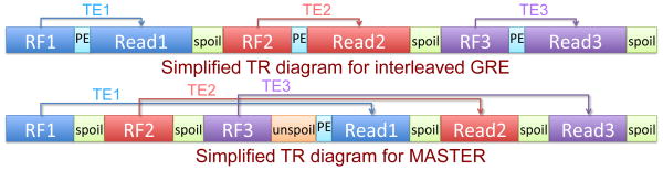
Simplified sequence diagram for interleaved GRE (top) and MASTER (bottom). RF excitation, readout, and TE are color-coded by slice number, “spoil” (green) is excitation defocusing, “unspoil” (orange) is excitation refocusing, and “PE” (cyan) is phase encoding.

A. Background

In order to excite multiple slices simultaneously but measure each independently, it is necessary to separate them in k-space. Instead of using a refocusing gradient after RF excitation to re-center k-space on a newly excited slice, MASTER uses additional gradient area after the slice selection to defocus the excitation by shifting the excited magnetization away from the k-space origin. After all of the slices have been excited, any slice can be re-centered at the k-space origin for read out. This is achieved with refocusing gradients that cancel the gradient area accrued since excitation for that slice. This spoiling and un-spoiling approach will be referred to here as excitation defocusing and excitation refocusing. This approach to multi-slice imaging was first introduced in the MUSIC sequence [26]. As will be seen, our approach differs from MUSIC in a few key ways.

B. Gradient Design Considerations

Excitation defocusing and refocusing gradients must generate sufficient k-space separation between excitations to avoid inter-slice interference without introducing excessive diffusion weighting. In the introductory MUSIC paper, all of the gradient shifts are along the readout dimension, which can cause significant signal loss due to diffusion. In MASTER, excitation defocusing and refocusing utilize all three gradient dimensions to reduce diffusion weighting as compared to MUSIC, by following a “coiling” trajectory in k-space (Fig. 2). The coiling pattern keeps magnetization closer to the k-space origin for reduced diffusion weighting, while maintaining sufficient separation between excited slices to avoid inter-slice interference.

Fig. 2.

Example k-space coiling trajectory for MASTER. Blocks indicate excited slices, red arrows indicate trajectory of defocusing gradients between excitations or refocusing gradients between readouts.

The amount of defocusing necessary to avoid measurable interference depends on imaging parameters and the object being imaged, so it must be determined based on a specific application. Increasing defocusing will decrease inter-slice interference while increasing sequence time and diffusion weighting. Due to the large total gradient areas involved, nonlinearities (due to eddy currents or other effects) can accrue and reduce imaging quality. To help nonlinear gradient errors cancel out, MASTER can be implemented with fixed refocusing offsets of different polarity, generating the grid pattern seen in the k_x-k_y coiling pattern in Fig. 2. By finishing the sequence at a single grid offset from the starting slice, the amount of time taken to refocus the first excitation is minimized. Finally, it is important to limit the slew rates used to avoid peripheral nerve stimulation.

III. Methods

The MASTER sequence was implemented on a 3T GE Signa 750 scanner using developmental builds SpinBench and RTHawk (HeartVista, Inc. Menlo Park, CA USA) [27]. A single-channel GE head coil was used for transmit and receive in the initial validation experiment, and the body coil was used for the subsequent comparison experiments. All analysis was performed using MATLAB (The Mathworks, Inc. Natick, MA USA).

As an estimate of the minimum necessary gradient defocusing area to avoid inter-slice interference, a simple GRE sequence was used to image a GE grid phantom with different amounts of k_z offset. At a k_z offset of 6.66 cycles/cm, measurements at a k_x offset of 5 cycles/cm were similar in magnitude to the noise floor. A conservative minimum diffusion offset of 7.5 cycles/cm in k_z and 15 cycles/cm in k_x or k_y was used in all of the work presented here.

A. Design Trade-off Simulation

Simulated curves comparing the theoretical temperature uncertainty vs update rate for different implementations of interleaved GRE and of MASTER were generated, to illustrate the design frontiers for the two sequences. Temperature uncertainty was defined as the standard deviation (from noise) in the temperature measurement, which was scaled from the standard deviation of the phase assuming α = 0.01 ppm/°C. For interleaved GRE, different realizable sampling rates (500 kHz / integer) were used to calculate readout duration, and then timing parameters for minimum length sequences were generated assuming 1.068 ms spoiling time and 0.724 ms excitation time. Readout bandwidths from 7.14kHz to 500 kHz were simulated. For MASTER sequences with multiple slices (single slice is GRE), it was assumed that RF and defocusing takes 2.05 ms per slice, refocusing gradients each take 1.53 ms, and spoiling takes 5.4 ms. These timing parameters were estimated from initial MASTER implementations, but will vary in actual implementations. Again, minimum duration sequences were simulated for different readout bandwidths. Different slices of the MASTER sequence will have different measurement accuracy, and only the median uncertainties are plotted in the results. In both simulations, 128 phase encodes were assumed (for a 256×128 matrix in each slice).

An initial simulation point of 1.3°C uncertainty for TE/TR/RBW = 12.8ms/27.66ms/11.36kHz was chosen based on measurements of a previously collected in vivo temperature sequence during a patient treatment. Uncertainty for other sequences was extrapolated based on TE/TR/RBW using T1 = 1097 ms, T2* = 50 ms, T2 = 70 ms. Choice of a different starting point would scale all simulated uncertainties linearly. Losses from diffusion and from imperfect gradient refocusing were not simulated, so the simulated results may be optimistic for many-slice MASTER sequences with larger defocusing and refocusing gradient area.

B. Validation Data Acquisition

To verify that the sequence can work in practice, and to see how image quality is impacted by the MASTER gradients, a six slice MASTER sequence was implemented. The sequence was designed to collect 6 slices in 5 seconds, and used the k-space coiling design shown in Fig. 2. This implementation will be referred to as “MASTER_6”. Additional sequence parameters are listed in Table I. The pulse sequence waveforms for MASTER_6 are shown in Fig. 3. Diffusion b-values ranged from 2.6 to 7.7 mm²/s, so expected signal loss in free water is less than 2%.

Table I. Sequence Parameters for Implemented MASTER_6 and GER_equiv Validation Sequences. TE Values Ordered from First to Last Slice.

	MASTER_6	GRE_equiv
TE (ms)	13.9, 15.1, 17.3, 18.0, 19.3, 21.5	17.0
TR (ms)	39.5	39.2
# Slices	6	1
Tip (°)	14.1	14.1
Slice Thickness	3 mm	3 mm
Slice Offsets	-30, -20, -10, 0, 10, 20 mm	0 mm
FOV	28 cm	28 cm
Matrix	256×128	256×128
ROBW	125 kHz (488 Hz/pixel)	125 kHz (488 Hz/pixel)

Fig. 3. Pulse sequence waveforms for MASTER_6.

In order to compare MASTER with GRE, a single slice GRE sequence was implemented with sequence parameters similar to the center (fourth) slice of the MASTER sequence. This sequence will be referred to as “GRE_equiv” and its parameters are also listed in Table I. Each of the implemented sequences used gradient spoiling.

The two sequences were used to measure temperature changes in a stationary unheated agar gel ball phantom. The sequences were also used to scan a healthy volunteer under IRB approval. At least 10 frames of data were collected in each scenario, and the first two frames of each data set were discarded to ensure that steady state was reached for all analyzed frames. Temperature changes were reconstructed by performing complex division of consecutive frames, converting the resulting phase difference into temperature based on TE. For each temperature update frame, 0^th order offset was measured in high SNR regions (voxels with at least half of the maximum magnitude among MASTER slices) and then subtracted to remove drift bias. Temperature uncertainty was measured for each voxel by taking the standard deviation across time of the temperature change data. Average temperature uncertainty for each slice was computed as the spatial average across the high SNR voxels.

C. Three Slice Sequence Comparison

To enable a direct comparison of interleaved GRE and MASTER, 3 slice sequences were designed with each approach to obtain three slices with minimum temperature uncertainty in 5 seconds. (Keeping with the previous convention, these sequences will be referred to as GRE_3 and MASTER_3.) Each sequence used both RF spoiling and gradient spoiling. Sequence parameters for these two sequences are listed in Table II. Diffusion b-values were less than 5 mm²/s. A healthy volunteer was scanned using each sequence, to obtain in vivo uncertainty comparisons. Temperature calculations were the same as for the validation sequences. To compare uncertainty between the two sequences, an ROI that did not include ventricles was selected for each slice, and temperature uncertainty was averaged within those ROIs.

Table II. Sequence Parameters for 3 Slice MASTER and GRE Validation Sequences. TE Values Ordered from First Slice to Last Slice.

	GRE_1	MASTER_3	GRE_3
TE (ms)	14.2	13.4, 20.6, 27.8	6.9, 6.9, 6.9
TR (ms)	28.2	40.9	41.9
# Slices	1	3	3
Tip (°)	30	30	30
Slice Thickness	3 mm	3 mm	3 mm
Slice Offsets	0 mm	-10, 0, 10 mm	-10, 0, 10 mm
FOV	28 cm	28 cm	28 cm
Matrix	256×128	256×128	256×128
ADBW	11.36 kHz (44.4 Hz/pixel)	31.25 kHz (122 Hz/pixel)	25 kHz (97.7 Hz/pixel)

D. Phantom Heating Experiment

The 3 slice sequences, along with a single slice GRE sequence (‘GRE_1’ with parameters listed in Table II), were used to measure temperature while heating a focal spot in a phantom. A HIFU phantom was heated using the Exablate 2000 system (Insightec, Haifa, Israel) with three sonications. Each sonication was 30 seconds long, using 32.4 W acoustic power, and the phantom was allowed to cool down for 15 minutes between sonications. The first heating was monitored with GRE_3, the second with MASTER_3, and the third with GRE_1. The MRI acquisition was not synchronized with the sonication, so the last frame that did not show a temperature rise was treated as time 0 for each heating. Temperature was calculated using the frames before heating as a baseline for each sequence/sonication. Peak measured temperature was located for each sequence, and images were re-centered around that voxel.

IV. Results

A. Design Trade-off Simulation Results

Fig. 4 shows the simulated design curves for multi-slice interleaved GRE and Fig. 5 shows the same trade-off for multi-slice MASTER. Acquisition time is the total amount of time to collect a fully sampled set of data, and would be the rate at which temperature measurements could be updated during treatment. Different simulation points along each curve used different sampling bandwidth, with TR minimized for that bandwidth. These curves are meant to show how the design frontier trades off uncertainty and time for MASTER and interleaved GRE for different numbers of slices.

Fig. 4. Simulated temperature measurement uncertainty vs acquisition duration for multi-slice interleaved GRE.

Fig. 5. Simulated median temperature measurement uncertainty vs acquisition duration for MASTER.

B. Validation Images and Uncertainty

To compare image quality and temperature measurement uncertainty between MASTER_6 and GRE_equiv, Fig. 6 shows a single frame of magnitude data and the temperature uncertainty through time in the agar gel phantom. Fig. 7 shows the same comparison in vivo. In each figure, only the center (fourth) slice of the MASTER_6 sequence is shown, to which the parameters of GRE_equiv were matched.

Fig. 6. Magnitude and temperature uncertainty in agar gel: MASTER_6 vs GRE_equiv.

Fig. 7. Magnitude and temperature uncertainty in vivo: MASTER_6 vs GRE_equiv.

For a quantitative comparison, the temperature uncertainty for the center slice of MASTER_6 was compared with that of GRE_equiv. Only voxels with at least half of the maximum signal intensity within the MASTER slice were included in the average. In phantom, the average temperature uncertainty for MASTER_6 was 0.269°C while it was 0.284°C for GRE_equiv. In vivo, average temperature uncertainty was 0.712°C for MASTER_6 and 0.681°C for GRE_equiv. Temperature uncertainty across the six slices of MASTER_6 are listed in Table III, along with the measured SNR in vivo. SNR was defined as mean signal magnitude divided by the standard deviation of noise in either the real or imaginary channel.

Table III. Performance for Each Slice of MASTER_6.

Slice #	1	2	3	4	5	6
Uncertainty in phantom (°C)	0.351	0.315	0.285	0.269	0.261	0.254
Uncertainty in vivo (°C)	0.767	0.714	0.760	0.712	0.694	0.735
SNR in vivo	12.4	11.9	10.5	10.1	9.4	8.6

To show the spatial variation of magnitude and uncertainty ple slices, magnitude of all slices from a single MASTER_6 in vivo data is shown in Fig. 8, while uncertainty for those slices is shown in Fig. 9. uncertainty is expected to vary with TE, TE for each slice is labeled in Fig. 9.

Fig. 8. Magnitude Images for Single Frame of MASTER_6 in vivo.

Fig. 9. Temperature uncertainty for MASTER_6 in vivo.

C. Three Slice Sequence Comparison Results

Images of temperature uncertainty in vivo for MASTER_3 and GRE_3 are shown in Fig. 10, zoomed to a 13.7×17.9 cm FOV. The ROIs used to average temperature uncertainty are shown with black boxes. Average temperature uncertainties were {0.89°, 0.78°, 0.80°} for MASTER_3 and {1.24°, 1.22°, 1.18°} for GRE_3. These values indicate that GRE_3 has {39%, 56%, 47%} higher temperature uncertainty than MASTER_3. Diffusion losses are expected to be less than 1%, based on MASTER_3 b values.

Fig. 10. Temperature uncertainty for MASTER_3 and GRE_3 in vivo, zoomed to show detail. Black boxes indicate ROIs used for temperature uncertainty average.

D. Phantom Heating Results

Temperature results from the phantom heating experiment are shown in Fig. 11-12. Fig. 11 shows the temperature measurements for each of the three sequences at the time closest to 19°C heating (the point on the heating curve closest to acquired sample times for the three sequences). The top row of images are cuts through the cylindrical phantom, trimmed to an 11.1 cm FOV. To compare focal heating, zoomed-in images of the hot spot are shown for each sequence, with zero-fill upsampling to 0.55mm isotropic voxel spacing. Full-width half-maximum heating in the frequency encode direction was consistent across sequences, with ±2% variation.

Fig. 11. Temperature maps during heating for three sequences, bottom row is zoomed to hot spot and upsampled.

Fig. 12.

Evolution of focal spot temperature in phantom, using three sequences to monitor three subsequent sonications. Red curves are focal slice, other curves are adjacent slices.

Fig. 12 shows the time course of the maximally heated voxel for each sequence, with a pink box estimating the duration of sonication. The red curves show the center (targeted) slice, while the green and blue curves are the adjacent slices. Peak measured temperatures (with average uncertainty calculated in non-heated regions) were: 24.3±0.58°C for GRE_1, 25.3±0.96°C for GRE_3, and 24.0±0.38°C for MASTER_3.

V. Discussion

A novel approach to multiple-slice thermometry was introduced in this work, an initial implementation was used to demonstrate its viability, and a direct comparison between MASTER and interleaved GRE was made for three slice acquisition. By exciting all slices before read out instead of reading each slice immediately after excitation, greater TEs are achievable than for traditional interleaved approaches, and temperature accuracy is improved. Images collected in phantom and in vivo show that MASTER achieves similar image quality and measurement accuracy when compared to interleaved GRE using the same timing parameters. MASTER obtains high temperature SNR while using high sampling bandwidths, so geometric fidelity is preserved in the presence of off-resonance.

A. Validation Comparison and Moving Fluid Insensitivity

The MASTER_6 and GRE_equiv validation images in pm are extremely similar qualitatively, with average temperature uncertainty differing by less than 6%. As expected, magnitude SNR decreased with increasing TE, while temperature precision increased, for the phantom measurements. However, the in vivo measurements showed less clear trends in temperature uncertainty, with slice 6 showing slightly higher uncertainty than predicted. Because the parameters are matched between the sequences, with MASTER adding additional gradients that may degrade image quality, the images being identical is the best-case scenario. The in vivo images reveal differences between the two sequences, though their average temperature uncertainty still matched to within 5%. In particular, CSF along the midline and blood in the sagittal sinus are not visible in the MASTER sequence. A loss in signal from moving fluids is an expected result from the defocusing and refocusing gradients in MASTER. The loss of signal from moving fluid leads to an increase in the standard deviation of temperature measurements in voxels that contain both brain tissue and fluid. However, the actual measurement of tissue temperature may be improved as compared to GRE despite a loss of signal, since the signal from the moving fluid will not confound the tissue temperature measurement.

B. Three Slice Comparison with Interleaved GRE

The MASTER_3 sequence and GRE_3 sequence were both designed to achieve the same objective (3 slices in 5 seconds), and serve as a direct comparison to show the performance advantage offered by MASTER for a small number of slices. In vivo, temperature uncertainty was 39%-56% higher using interleaved GRE than using MASTER to acquire 3 slices in 5 seconds. The advantage of using MASTER will increase for more slices or for faster sequences as shown in Figs. 4-5. The simulation curves over-predict absolute uncertainty values, since they were estimated from data collected during a clinical treatment while these results were obtained without a transducer or water bath present, but relative performance between the sequences is consistent. Uncertainty in the third slice of MASTER_3 was larger than expected, just as the last slice in MASTER_6 showed unexpectedly high variation. This caused median uncertainty to be slightly less improved experimentally than was predicted by simulation. This may be inherent signal loss due to the MASTER gradients, or it may result from imperfect gradients (due to eddy currents) not yielding perfect refocusing.

Measured temperature time courses during phantom heating experiments looked consistent across the three sequences. Temperature uncertainty was significantly smaller for MASTER_3 than the other two sequences, but T2* values in the phantom are longer than those in the brain and exaggerate the benefit of longer TEs. Peak measured temperature was slightly higher for the GRE_3 sequence, which could reflect a difference in the actual temperature achieved during the different sonications, a difference in timing of the measurements relative to peak heating, or be due to noise. Alternatively, the linear coefficient relating phase and temperature might be TE-dependent, as proposed in [28]. There was no significant difference in temperature resolution between the sequences, based on the measured heat profiles.

C. Slice-Dependent TEs and Update Rates

While the MUSIC sequence uses a fixed TE for all slices, MASTER seeks to maximize efficiency by minimizing all gradient durations and dead time. This maximizes the amount of time during the sequence that can be spent on readout, increasing the SNR for any given update rate. Because the amount of time necessary to excite and defocus a slice may be different than the amount of time necessary for refocusing and readout, each slice can have a different TE and therefore different temperature SNR. If a particular application requires constant TE across slices, then dead time can be added to make the TE constant. In typical thermometry applications, maximum efficiency is most important, and the ordering of the slices within the sequence can be selected such that the highest priority slices (where heating is expected) have the highest SNR (generally the longest TE). Alternatively, if some slices have shorter T2* than others, for instance due to proximity to the sinuses, these slices could be assigned shorter TEs to improve overall accuracy.

While the targeted focal spot will heat quickly and requires fast temperature measurements, background regions can be monitored more slowly and still benefit patient safety. With the MASTER sequence, different slices can be updated at different rates, by only measuring them at integer multiple TRs. If a slice is only excited every second (or third…) TR, steady state will still be attained. With this approach, important slices can be updated as fast as possible while monitoring a larger volume outside the treatment zone with slower update rates. Phase encoding will remain constant across all slices in each TR, and RF amplitude for the slow slices can be increased to maintain the Ernst angle for their longer effective TRs. When alternating between two slices with a particular excitation of the sequence, those two slices will each update simultaneously every other time the fast slices update, and will have a higher SNR than the fast update slices due to their longer effective TR.

D. Application-Specific Sequence Design

MASTER opens up a large new design space for trading off volume, update rate, and accuracy of temperature monitoring. However, the specific needs and tradeoffs of different applications necessitate different sequence designs for maximum benefit. During the planning stage of brain treatments, it is necessary to verify that the ultrasound focal point is located in the proper part of the anatomy. For this application, a small number of slices located around the expected focal point are sufficient, and temporal restrictions are not as stringent. When imaging contiguous slices, slice profile requirements will be stricter to avoid inter-slice interference. During treatment, a larger number of slices would allow for background monitoring, and the background slices could be collected at a lower frame rate than the slices covering the treatment region. These two stages of the same clinical application would desire very different implementations of MASTER, and different trade-offs will exist for other applications.

Other imaging applications that desire long TE measurements with multiple slices and fast imaging update rates could benefit from using MASTER. One possible application, which was targeted with the MUSIC sequence, is fMRI. In functional imaging, it is important to see the full brain with high temporal resolution (faster than 3 seconds per frame), and BOLD contrast is maximized at TE=T2*. As compared to single-shot fMRI techniques, MASTER may allow for shorter readouts and reduction of imaging artifacts while maintaining full brain coverage and usable accuracy and speed. Dead time could be added to the sequence to equalize TE across slices and give consistent activation amplitudes, or a reference T2* image could be acquired before scanning to convert each slice's measured signal change into estimated T2* percent change for fMRI.

E. Acceleration, and Further Design Improvements

While the design curves for multiple slice MASTER have become significantly faster when compared to interleaved GRE, additional improvement is necessary to collect more than a few slices with clinically acceptable speed and accuracy. For further improvement, multiple acceleration techniques are possible. Using non-Cartesian sampling trajectories, such as EPI or spiral, can reduce the number of TRs necessary for a full image. With fewer TRs, longer TEs and TRs could be used for a given update rate, increasing SNR. Additionally, a larger fraction of the sequence time would be spent recording signal, increasing sequence efficiency. However, readouts must remain short to avoid imaging artifacts. Parallel imaging and compressed sensing approaches that accelerate traditional GRE sequences should be fully applicable to MASTER data. By combining nonlinear trajectories with these acceleration techniques, more slices can be acquired within clinically acceptable speed and accuracy constraints.

References

- 1.Martin E, Jeanmonod D, Morel A, Zadicario E, Werner B. High-intensity focused ultrasound for noninvasive functional neurosurgery. Ann Neurol. 2009 Dec;66(6):858–61. doi: 10.1002/ana.21801. [DOI] [PubMed] [Google Scholar]
- 2.Jeanmonod D, Werner B, Morel A. Transcranial magnetic resonance imaging–guided focused ultrasound: noninvasive central lateral thalamotomy for chronic neuropathic pain. Neurosurg Focus. 2012;32(January):1–11. doi: 10.3171/2011.10.FOCUS11248. [DOI] [PubMed] [Google Scholar]
- 3.McDannold N, Clement G, Black P. Transcranial MRI-guided focused ultrasound surgery of brain tumors: Initial finding in three patients. Neurosurgery. 2010;66(2):323–332. doi: 10.1227/01.NEU.0000360379.95800.2F. [DOI] [PMC free article] [PubMed] [Google Scholar]
- 4.Elias WJ, et al. A Pilot Study of Focused Ultrasound Thalamotomy for Essential Tremor. N Engl J Med. 2013 Aug;369(7):640–648. doi: 10.1056/NEJMoa1300962. [DOI] [PubMed] [Google Scholar]
- 5.Todd N, Vyas U, de Bever J, Payne A, Parker DL. The effects of spatial sampling choices on MR temperature measurements. Magn Reson Med. 2011 Feb;65(2):515–21. doi: 10.1002/mrm.22636. [DOI] [PMC free article] [PubMed] [Google Scholar]
- 6.McDannold N, King RL, Hynynen K. MRI monitoring of heating produced by ultrasound absorption in the skull: in vivo study in pigs. Magn Reson Med. 2004 May;51(5):1061–5. doi: 10.1002/mrm.20043. [DOI] [PubMed] [Google Scholar]
- 7.Hynynen K, Sun J. Trans-skull ultrasound therapy: the feasibility of using image-derived skull thickness information to correct the phase distortion. IEEE Trans Ultrason Ferroelectr Freq Control. 1999 Jan;46(3):752–5. doi: 10.1109/58.764862. [DOI] [PubMed] [Google Scholar]
- 8.Sun J, Hynynen K. The potential of transskull ultrasound therapy and surgery using the maximum available skull surface area. J Acoust Soc Am. 1999 Apr;105(4):2519–27. doi: 10.1121/1.426863. [DOI] [PubMed] [Google Scholar]
- 9.Bitton RR, Pauly KRB. MR-acoustic radiation force imaging (MR-ARFI) and susceptibility weighted imaging (SWI) to visualize calcifications in ex vivo swine brain. J Magn Reson Imaging. 2013 Oct;00:1–7. doi: 10.1002/jmri.24255. [DOI] [PMC free article] [PubMed] [Google Scholar]
- 10.Ishihara Y, Calderon A, Watanabe H, Okamoto K, Suzuki Y, Kuroda K. A precise and fast temperature mapping using water proton chemical shift. Magn Reson Med. 1995 Dec;34(6):814–23. doi: 10.1002/mrm.1910340606. [DOI] [PubMed] [Google Scholar]
- 11.Rieke V, Butts Pauly K. MR thermometry. J Magn Reson Imaging. 2008 Feb;27(2):376–90. doi: 10.1002/jmri.21265. [DOI] [PMC free article] [PubMed] [Google Scholar]
- 12.Quesson B, a de Zwart J, Moonen CT. Magnetic resonance temperature imaging for guidance of thermotherapy. J Magn Reson Imaging. 2000 Oct;12(4):525–33. doi: 10.1002/1522-2586(200010)12:4<525::aid-jmri3>3.0.co;2-v. [DOI] [PubMed] [Google Scholar]
- 13.Yuan J, Mei CS, Panych L, McDannold NJ, Madore B. Towards fast and accurate temperature mapping with proton resonance frequency-based MR thermometry. Quant Imaging Med Surg. 2012 Jan;2(1):21–32. doi: 10.3978/j.issn.2223-4292.2012.01.06. [DOI] [PMC free article] [PubMed] [Google Scholar]
- 14.Rivens I, Shaw a, Civale J, Morris H. Treatment monitoring and thermometry for therapeutic focused ultrasound. Int J Hyperth. 2007 Jan;23(2):121–139. doi: 10.1080/02656730701207842. [DOI] [PubMed] [Google Scholar]
- 15.Peters RD, Hinks RS, Henkelman RM. Ex vivo tissue-type independence in proton-resonance frequency shift MR thermometry. Magn Reson Med. 1998 Sep;40(3):454–9. doi: 10.1002/mrm.1910400316. [DOI] [PubMed] [Google Scholar]
- 16.Cline HE, et al. Simultaneous magnetic resonance phase and magnitude temperature maps in muscle. Magn Reson Med. 1996 Mar;35(3):309–15. doi: 10.1002/mrm.1910350307. [DOI] [PubMed] [Google Scholar]
- 17.Sekihara K. Steady-State Magnetizations in Rapid NMR Imaging Using Small Flip Angles and Short Repetition Intervals. Med Imaging, IEEE Trans. 1987;MI(2) doi: 10.1109/TMI.1987.4307816. [DOI] [PubMed] [Google Scholar]
- 18.a de Zwart J, Vimeux FC, Delalande C, Canioni P, Moonen CT. Fast lipid-suppressed MR temperature mapping with echo-shifted gradient-echo imaging and spectral-spatial excitation. Magn Reson Med. 1999 Jul;42(1):53–9. doi: 10.1002/(sici)1522-2594(199907)42:1<53::aid-mrm9>3.0.co;2-s. [DOI] [PubMed] [Google Scholar]
- 19.Roujol S, Ries M, Quesson B, Moonen C, Denis de Senneville B. Real-time MR-thermometry and dosimetry for interventional guidance on abdominal organs. Magn Reson Med. 2010 Apr;63(4):1080–7. doi: 10.1002/mrm.22309. [DOI] [PubMed] [Google Scholar]
- 20.Köhler MO, Mougenot C, Quesson B, Enholm J, Le Bail B, Laurent C, Moonen CTW, Ehnholm GJ. Volumetric HIFU ablation under 3D guidance of rapid MRI thermometry. Med Phys. 2009;36(8):3521. doi: 10.1118/1.3152112. [DOI] [PubMed] [Google Scholar]
- 21.Quesson B, et al. Real-time volumetric MRI thermometry of focused ultrasound ablation in vivo: a feasibility study in pig liver and kidney. NMR Biomed. 2011 Feb;24(2):145–53. doi: 10.1002/nbm.1563. [DOI] [PubMed] [Google Scholar]
- 22.Mei CS, Afacan O, Yuan J, Madore B, Panych LP, McDannold NJ. Multi-shot high-speed 3D-EPI thermometry using a hybrid method combining 2DRF excitation, parallel imaging, and UNFOLD. 19th Scientific Meeting, International Society for Magnetic Resonance in Medicine; Montreal, Quebec. 2011. [Google Scholar]
- 23.Todd N, Vyas U, de Bever J, Payne A, Parker DL. Reconstruction of fully three-dimensional high spatial and temporal resolution MR temperature maps for retrospective applications. Magn Reson Med. 2012 Mar;67(3):724–30. doi: 10.1002/mrm.23055. [DOI] [PMC free article] [PubMed] [Google Scholar]
- 24.Madore B, Panych LP, Mei CS, Yuan J, Chu R. Multipathway sequences for MR thermometry. Magn Reson Med. 2011 Sep;66(3):658–68. doi: 10.1002/mrm.22844. [DOI] [PMC free article] [PubMed] [Google Scholar]
- 25.Farzaneh F, Riederer SJ, Pelc NJ. Analysis of T2 limitations and off-resonance effects on spatial resolution and artifacts in echo-planar imaging. Magn Reson Med. 1990 Apr;14(1):123–39. doi: 10.1002/mrm.1910140112. [DOI] [PubMed] [Google Scholar]
- 26.Loenneker T, Hennel F, Hennig J. Multislice interleaved excitation cycles (MUSIC): an efficient gradient-echo technique for functional MRI. Magn Reson Med. 1996 Jun;35(6):870–4. doi: 10.1002/mrm.1910350613. [DOI] [PubMed] [Google Scholar]
- 27.Santos JM, Wright GA, Pauly JM. Flexible real-time magnetic resonance imaging framework. Conf Proc IEEE Eng Med Biol Soc. 2004;2:1048–1051. doi: 10.1109/IEMBS.2004.1403343. [DOI] [PubMed] [Google Scholar]
- 28.Peters RD, Henkelman RM. Proton-resonance frequency shift MR thermometry is affected by changes in the electrical conductivity of tissue. Magn Reson Med. 2000 Jan;43(1):62–71. doi: 10.1002/(sici)1522-2594(200001)43:1<62::aid-mrm8>3.0.co;2-1. [DOI] [PubMed] [Google Scholar]