Investigation of BOLD fMRI resonance frequency shifts and quantitative susceptibility changes at 7 T

Abstract

Although blood oxygenation level dependent (BOLD) functional magnetic resonance imaging (fMRI) experiments of brain activity generally rely on the magnitude of the signal, they also provide frequency information that can be derived from the phase of the signal. However, because of confounding effects of instrumental and physiological origin, BOLD related frequency information is difficult to extract and therefore rarely used. Here, we explored the use of high field (7 T) and dedicated signal processing methods to extract frequency information and use it to quantify and interpret blood oxygenation and blood volume changes. We found that optimized preprocessing improves detection of task‐evoked and spontaneous changes in phase signals and resonance frequency shifts over large areas of the cortex with sensitivity comparable to that of magnitude signals. Moreover, our results suggest the feasibility of mapping BOLD quantitative susceptibility changes in at least part of the activated area and its largest draining veins. Comparison with magnitude data suggests that the observed susceptibility changes originate from neuronal activity through induced blood volume and oxygenation changes in pial and intracortical veins. Further, from frequency shifts and susceptibility values, we estimated that, relative to baseline, the fractional oxygen saturation in large vessels increased by 0.02–0.05 during stimulation, which is consistent to previously published estimates. Together, these findings demonstrate that valuable information can be derived from fMRI imaging of BOLD frequency shifts and quantitative susceptibility changes. Hum Brain Mapp 35:2191–2205, 2014. © 2013 Wiley Periodicals, Inc.

INTRODUCTION

The use of the phase of magnetic resonance imaging (MRI) signals has proven very useful to investigate human brain anatomy because of the increased contrast between and within the gray and the white matter, and the information it provides complementary to magnitude signals for quantification purposes [Duyn et al., 2007].

In functional MRI (fMRI), phase in part reflects blood susceptibility, whose changes form the basis of the blood oxygenation level dependent (BOLD) effect on magnitude fMRI signals. The complementary information it contains could potentially be used to untangle changes in blood fractional oxygen saturation from changes in blood volume. Blood fractional oxygen saturation is an indicator of oxygen delivery and metabolism, and may provide information about tissue function and viability. Current methods employed to estimate changes in the blood fractional oxygen saturation rely on the use of sophisticated fMRI acquisition sequences and modeling methods [He and Yablonskiy, 2007] or of invasive procedures such as positron emission tomography [Ito et al., 2005].

Nevertheless, unlike in structural imaging, the use of phase in fMRI has been very limited so far, primarily because of difficulties of its extraction and interpretation. Phase‐based fMRI activity maps have had limited signal‐to‐noise ratio and only show robust changes with brain activation in the larger veins [Menon, 2002; Nencka and Rowe, 2007]. A problem with phase‐based fMRI is the presence of large instrumental and physiological noise fluctuations over time that obscure changes related to neuronal activity [Petridou et al., 2009; Hagberg et al., 2012]. Previous attempts at reducing noise in phase fMRI have included the use of noise regressors derived from physiological monitoring [Petridou et al., 2009], the application of spatial high‐pass filters [Hagberg et al., 2012], or correction of the estimated frequency offsets with the simulated phase rewinding method [Hahn et al., 2009].

In this work, we aimed at improving the acquisition and processing of phase‐based fMRI activity time‐courses. For this purpose, we used advanced technology (7 T scanner, array detectors) and optimized preprocessing to account for instrumental and physiological noise in phase fMRI images acquired during stimulation and at rest. Crucially, we removed the background spatial low‐frequency phase variation by subtracting spatially fitted polynomials on a slice‐by‐slice basis, and examined the residual BOLD changes in the phase time‐course. Further, we computed BOLD frequency shifts from phase values, and estimated quantitative susceptibility changes in the activated area and large draining veins (for instance the sagittal sinus) using methods developed previously for structural susceptibility imaging. Finally, in an initial application, we aimed at estimating the functional change in blood fractional oxygen saturation in large veins during task performance from BOLD frequency shifts and susceptibility values computed from phase signals. Part of this work was previously published in abbreviated abstract form (Bianciardi et al., 2011a; Bianciardi et al., 2012).

METHODS

Experimental Design

Groups of eight (four males, four females, age 30 ± 3 years, Experiment 1) and six healthy subjects (three males, three females, 33 ± 3 years, Experiment 2) participated in two separate experiments, after giving written informed consent. The human subject protocol was approved by the Institutional Review Board (IRB) of the National Institutes of Health (NIH).

The first experiment (Experiment 1) was performed to investigate if small BOLD phase signal changes can be untangled from confounding noise contributions by optimized preprocessing, and to study the signal change dependence on echo time; in the second experiment (Experiment 2), we studied the feasibility of computing quantitative BOLD susceptibility changes from phase signal changes.

Two conditions were investigated: (1) visual fixation on a central dot during presentation of a visual stimulus (black/white checkerboard, flickering at 7.5 Hz, block‐design: 34.5 s OFF/34.5 s ON cycle); (2) resting with the eyes closed.

Image Acquisition

In Experiment 1, multi gradient‐echo (GRE) echo‐planar imaging (EPI) BOLD‐fMRI was performed on a 7 T General Electric Signa MRI scanner (GE‐Medical‐Systems, Waukesha, WI), using a 32 channel receive‐only coil (Nova Medical, Wilmington, MA) and parameters: echo times (TEs) = [15.0, 31.5, 48.0, 64.5, 81.0] ms, repetition time (TR) = 2.3 s, flip angle = 65°, number of slices = 4, slice orientation = oblique axial/coronal (rotation angle with respect to axial orientation ranging between 7° and 33° across subjects), voxel‐size = 2.5 × 2.5 × 2.5 mm³, field of view = 240 × 180 mm², number of scans = 158, SENSE rate = 3. Considering an in vivo measured blood T ₁ of ∼ 2.6 s at 7 T [Rooney et al., 2007], the chosen flip angle (65°) maximizes signal (Ernst angle) for the blood compartment. This is slightly suboptimal for gray matter (a cortical gray matter T ₁ of ∼ 2.1 s, Rooney et al., 2007, yields an Ernst angle of 70.4°). Nevertheless, the conservative low value of the target flip angle may prevent signal loss in regions with B1 hot spots typical of high field MRI. In Experiment 2, data coverage in the z‐direction was increased to facilitate the calculation of magnetic susceptibility from phase data. For this purpose, the same GRE‐EPI parameters as in Experiment 1 were employed except for: TEs = 31.5 ms, number of slices = 40, slice orientation = coronal. The first image was acquired with flip angle set to zero to estimate coil noise levels for image reconstruction. Scans 2–4 (approach to steady‐state) were discarded and scans 5–7 were used as reference for coil sensitivity mapping. Remaining scans were used for brain activity analysis. Head motion was minimized by the use of foam pads, placed in the space between the interior coating of the MRI detector array and the subject's head.

A high‐resolution gradient‐recalled echo image was also acquired (TE = 16 ms, voxel size = 0.3125 × 0.3125 × 2.5 mm³, TR = 1.2 s, flip angle = 70°, same number of slices and slice orientation of GRE‐EPI images). Real‐time modulation of B ₀ shims up to the second order was applied to compensate for large‐scale B ₀‐field fluctuations induced in the head by respiration [van Gelderen et al., 2007]. This was carried out on average across the brain, and finer spatial scale was removed retrospectively (see next paragraph). We also recorded the timing of physiological cycles by the use of a pulse‐oximeter and respiratory bellow provided with the MR scanner, at a sampling rate of 250 Hz.

Magnitude and Phase Image Processing

Data processing for Experiments 1 and 2 differed only in a few details which are specified below.

In summary, for both Experiment 1 and 2, the data processing stream included: image reconstruction; phase data preprocessing; physiological and instrumental noise correction; slice timing, and spatial alignment of magnitude and phase data; computation of magnitude % signal changes and fractional frequency shifts; computation of stimulus‐related and resting state activity maps for magnitude, and phase data. In addition to the steps above, for Experiment 2 only, susceptibility changes were computed from fractional frequency shifts, and activity maps were computed for the obtained susceptibility changes.

For both experiments, multiple coil images were combined to yield complex images (off‐line SENSE image reconstruction), and then magnitude and phase images were computed (IDL 8.1, Exelis Visual Information Solutions, Boulder, CO).

For each TE and each voxel, phase images were preprocessed as follows (Matlab 7.13, The Mathworks, Natick, MA): the first value of the phase time‐course (Φ_t0) was subtracted from each time‐point (Φ_t), resulting in ΔΦ = Φ_t − Φ_t0; the phase time‐course was then unwrapped by assuming time‐continuity and the linear drift over time was removed. For each TE, the background spatial low‐frequency phase variation was fitted for each slice and for each time‐point with a spatial polynomial function (model orders 2, 4, 6, 8 were investigated). Spatial polynomial functions are also used during real time shimming [van Gelderen et al., 2007]. These signal fluctuations were attributed to drifts over time and to the respiratory chest motion (see Results and Table 1) and were employed, on a voxel‐by‐voxel basis, as noise regressor (Φnoise‐regressor) for both magnitude and phase fMRI data.

Table 1.

Variance (%) of the Φnoise‐regressor accounted by instrumental noise, physiological noise, and stimulus regressor

	ROIVC		ROIGM
	TASK	REST	TASK	REST
Drifts	30.10 (7.83)a	25.85 (7.04)	32.09 (8.59)	27.21 (7.49)
Respiratory cycleb	21.42 (4.90)	16.52 (6.77)	20.15 (6.05)	16.16 (6.74)
Cardiac cycle	1.00 (0.73)	0.32 (0.26)	1.65 (0.86)	0.59 (0.43)
Respiratory volume rate	0.67 (0.34)	2.42 (0.71)	0.89 (0.54)	2.44 (0.69)
Cardiac rate	0.86 (0.32)	1.67 (0.55)	0.81 (0.31)	1.59 (0.55)
Stimulus regressor	0.24 (0.12)	N/A	0.04 (0.08)	N/A
Residual noisec	45.71 (8.50)	53.22 (5.14)	44.37 (8.19)	52.01 (5.61)

^aMean (standard error) across six subjects of the average value across voxels of each ROI (VC = visual cortex, GM = gray matter).

^bFour RETROICOR regressors were used to model effects related to the phase of the respiratory cycle.

^cResidual noise might include thermal noise, noise related to motion correction (processing step applied afterwards), and residual uncorrected signal fluctuations due to instrumental noise, physiological noise, and task related neuronal processes.

Physiological and instrumental noise correction was then applied on both magnitude and pre‐processed phase images on a slice‐by‐slice basis, including five different noise sources, as follows. (1) Instrumental and physiological drifts over time were accounted for by third order polynomials; drifts over time might arise from several sources of instrumental (radiofrequency transmit/receive, gradient heating, field of superconducting magnet, etc.) instability [Smith et al., 1999] but also from physiological sources of instability [Yan et al., 2009]; drifts over time were therefore estimated from the regression coefficients of the polynomial fitting. (2) Effects of chest motion associated with the respiratory cycle were modeled with Φnoise‐regressor; the variance explained by Φnoise‐regressor was compared with that of four respiratory RETROICOR regressors [Glover et al., 2000], employed in previous work [Petridou et al., 2009] to reduce noise in phase fMRI signals. (3) Effects related to the phase of cardiac cycle were modeled with four cardiac RETROICOR regressors [Glover et al., 2000]. Signal fluctuations due to change in (4) the respiratory volume rate and (5) cardiac rate [Birn et al., 2006; Shmueli et al., 2007] were accounted for by a dual‐lagged model [Bianciardi et al., 2009, 2011b; lags = −2.3 s and +11.5 s for respiration volume rate regressor, and −2.3 s and +4.6 s for cardiac rate regressor]. RETROICOR, respiration volume rate and cardiac‐rate regressors were estimated from physiological recordings according to strategies described respectively in Glover et al., 2000, Birn et al., 2006, and Shmueli et al., 2007. For magnitude images, physiological and instrumental noise was regressed out using a design matrix comprising noise regressors 1–5. For phase images, noise source (2) was first subtracted and then noise sources (1), (3)–(5) regressed out. For Experiment 1, full physiological and instrumental noise correction as explained above was performed for six subjects only, because for two subjects, for technical reasons, real‐time shimming did not run and physiological recordings were not saved. For these two subjects, only drifts and Φ noise‐regressor were regressed out.

Before further preprocessing was applied, for Experiment 1 we evaluated the contribution of each noise regressor to magnitude and phase signal fluctuations, and in particular we compared the performance of Φ noise‐regressor to that of four respiratory RETROICOR regressors as model for noise source (2). To this end, we estimated the variance each noise regressor explained in a region of interest in the visual cortex (ROI_VC) and in the gray matter (ROI_GM). ROI_VC was defined from the task activation data by thresholded correlation of the magnitude images (TE = 31.5 ms) with a stimulus regressor (P < 0.05 Bonferroni corrected, both positive and negative activations). This was done after running the preprocessing [instrumental/physiological noise correction included only noise source (1) to avoid bias in the comparison of different correction procedures employed for noise source (2)]. ROI_GM was identified [see also Bianciardi et al., 2009] from thresholded correlation with the whole brain signal (P < 0.05 Bonferroni corrected). For the noise source estimation, a set of nested design matrices [see Bianciardi et al., 2009 for details] was used including noise sources (1)–(5). The variance explained by each noise source was computed at the voxel level as the difference between the coefficients of determination adjusted by the degrees of freedom of two consecutive regression models, multiplied by 100. The stimulus regressor was included as an additional source of variance for the stimulus session only.

After physiological and instrumental noise correction, further processing of magnitude and phase fMRI data included: slice‐timing (by FMRIB Software Library, FSL4.1, Oxford, UK), motion correction (by custom routines implemented in IDL 8.1 software, Exelis Visual Information Solutions, Boulder, CO), and co‐registration between different volumes (FSL4.1). Finally, fluctuations in signal magnitude were converted to % signal changes relative to their time average (M/M ₀, %) by dividing the signal at each time point by the mean signal across time. Fractional frequency shifts (Δω/ω ₀, ppm) were computed from phase signal changes (ΔΦ = Φ_t − Φ_t0) according to: Δω/ω ₀ = (ω _t − ω _t0)/ω ₀ = −ΔΦ/(2π·γ _T B ₀TE) (γ _T B ₀ = 298 MHz; the minus sign before ΔΦ was used to restore the proper sign convention for frequency shifts on our MRI system).

For Experiment 2 only, susceptibility values Δχ (Δχ = χ _t − χ _t0) were computed for each voxel and time‐point from Δω/ω ₀ by means of Fourier‐based computation by a masked de‐convolution filter [Shmueli et al., 2009; Wharton et al., 2010], according to:

$$\{\begin{array}{l}\Delta \chi =\text{}FF{T}^{-1}\left[F\left(k\right)\cdot FFT\left(\Delta \omega /{\omega }_0\right)\right]\hfill \\ F(k)=1/\left(1/3-k_z^2/k^2\right)\hfill \end{array}$$ (1)

F(k) was set equal to 0 if |1/3 − k ² _z/k ²|< 0.3. Equation (1) was applied to data of Experiment 2 only (data volume rotation was not required because of coronal slice orientation). Importantly, the de‐convolution filter is a linear kernel, because both the direct and inverse Fourier transforms are linear functions; this means that the computed susceptibility changes (Δχ) on the left side of Eq. (1) represent the difference between the susceptibility at a certain time point (χ _t) and the susceptibility of the first time‐point (χ _t0) of the time‐course.

For a voxel containing a combination of capillaries, venules, and veins, the susceptibility difference during activation and baseline (Δχ _A‐B) is related to both blood fractional oxygen saturation (Y, range 0–1) and blood volume (CBV) changes according to:

$$\Delta {\chi }_{\text{A-B}}=\text{(}\Delta {\chi }_{\text{oxy-deoxy}}\text{Hct)}\cdot \text{(1}-{\mathrm{Y}}_{\mathrm{A}}\text{)}\cdot \Delta {\text{CBV}}_{\text{A-B}}-\Delta {\mathrm{Y}}_{\text{A-B}}\cdot {\text{CBV}}_{\mathrm{B}}$$ (2)

with Δχ _oxy‐deoxy the susceptibility difference between fully oxygenated and fully deoxygenated hemoglobin (0.18 ppm was employed, Weisskoff and Kiihne, 1992), Hct the hematocrit value (0.4 was used, Guyton and Hall, 2000), and the subscripts A and B representing the active and baseline states respectively.

Stimulus‐related activity maps of M/M ₀ and phase signals (or frequency shifts Δω/ω ₀ and for Experiment 2 only susceptibility changes Δχ) during stimulation were obtained by linear regression (Analysis of Functional Neuro Images (AFNI) tool, NIH, Bethesda, MD) of each voxel signal with a stimulus regressor (statistical threshold: P < 0.05 Bonferroni corrected). The stimulus regressor resulted from the convolution of stimulus functions (based on the timing of stimulation events) with the Statistical Parametric Mapping (SPM, London, UK) standard hemodynamic response function. M/M ₀ and phase spontaneous activity maps at rest were generated by computing the correlation of the average time series across voxels of the magnitude stimulus‐related activity map with the signal in each voxel, after temporal low‐pass filtering at f _C = 0.07 Hz (P < 0.05 Bonferroni corrected). The degrees of freedom were corrected for the number of noise regressors included in the preprocessing (stimulus and resting data), and for low‐pass filtering (resting data only).

For each TE and voxel, the amplitude of magnitude (Amplitude_M/M0) and phase (Amplitude_ΔΦ) signal fluctuations was computed as the signal standard deviation over time. The amplitudes of magnitude and phase signal fluctuations were fitted linearly with TE, according respectively to: Amplitude_M/M0 (%) ≅ −ΔR ₂* TE + Amplitude_M/M0 (TE = 0), and Amplitude_ΔΦ = −2π·γ _T B ₀ Δω/ω ₀ TE + Amplitude_ΔΦ (TE = 0) (ΔR ₂* is the transverse relaxation rate change).

Estimation of Changes in Fractional Oxygen Saturation in Large Veins

For Experiment 1, a voxel in the sagittal sinus was identified (see for example Figure 5B, blue arrow) by inspection of the high‐resolution GRE image. The average signal change in M/M ₀ (<ΔM _A‐B/M ₀>) and Δω/ω ₀ (<Δω _A‐B/ω ₀>) during stimulation (ON periods) with respect to baseline (OFF stimulation periods) was calculated.

Figure 5.

BOLD changes in magnitude (M/M ₀) and frequency shifts (Δω/ω ₀) signals in the sagittal sinus. For two subject participating in Experiment 1: (A) M/M ₀, and (B) Δω/ω ₀ activity maps (red/green = positive/negative correlation with stimulus regressor, P < 0.05 Bonferroni corrected) overlaid on a magnitude EPI image; (C) magnitude EPI image; (D) high‐resolution gradient‐recalled echo image; (E) Δω/ω ₀ and M/M ₀ time‐courses in the sagittal sinus (the sign of Δω/ω ₀ was inverted for display purposes only). The blue arrow indicates the location of the sagittal sinus. In subject 1 and 2, <ΔM _A‐B/M ₀> was = 10.5 and 11.0%; <Δω _A‐B/ω ₀> was = −2.4 and −2.6 ppb, yielding a <ΔY _A‐B> of 0.048 and 0.054, respectively.

Assuming a cylindrical vessel and no partial volume effects, the average change in fractional oxygen saturation during stimulation with respect to rest (<ΔY _A‐B>) was calculated from <Δω/ω ₀> as follows [Ogawa et al., 1993]:

$${\text{<ΔY}}_{\text{A-B}}\text{> = }\frac{1}{\left(\frac{1}{3}{\text{ - cos}}^2\text{θ}\right)}\cdot \frac{{\text{<Δω}}_{\mathrm{A}-\mathrm{B}}{\text{/ω}}_0\text{>}}{{\text{Δχ}}_{\text{oxy-deoxy}}\cdot \text{Hct}}$$ (3)

with: θ the angle between the vessel axis and B ₀, Δχ _oxy‐deoxy and Hct as in Eq. (2). Equation (3) assuming a cylindrical model was used only for large vessels and only for data of Experiment 1.

To overcome frequency shifts dependence on vessel orientation, we also computed changes in fractional oxygen saturation from susceptibility changes [as obtained from Eq. (1)] in Experiment 2 which provided extended brain coverage in the z‐direction. The average signal change in Δχ (<Δχ _A‐B>) during stimulation with respect to baseline was calculated in large vessels; assuming ΔCBV = 0, CBV_B = 1 in Eq. (2), <ΔY _A‐B> was then computed from <Δχ _A‐B> according to:

$${\text{<ΔY}}_{\text{A-B}}\text{> = -}\frac{{\text{<Δχ}}_{\mathrm{A}-\mathrm{B}}\text{>}}{{\text{Δχ}}_{\text{oxy-deoxy}}\cdot \text{Hct}}$$ (4)

RESULTS

Optimization of fMRI Phase Image Preprocessing

During calculation of the phase, each preprocessing step removed a substantial amount of temporal signal instability attributed to instrumental and physiological noise. As seen from comparing Figure 1B with A, after subtraction of the first phase image of the time‐series, voxel‐by‐voxel unwrapping over time and removal of linear drift over time, phase wraps over space and over time and very slow fluctuations are removed: note that the dynamic range of phase variation across one slice is decreased by an order of magnitude. Nevertheless, low frequency spatial variation of the phase remains, as judged from the amplitude and time course of the spatial polynomial fit (Fig. 1C, left and right panels respectively). This high temporal frequency variation follows the respiratory cycle (shown in Fig. 1C right panel, blue). After subtraction of spatially fitted polynomials, the resulting phase image is much more homogeneous (Fig. 1D, left panel), and the time‐course has a lower content of high temporal frequency fluctuation (Fig. 1D, right panel, black). The remaining phase variation resembles that of the magnitude time‐course (Fig. 1D, right panel, magenta) as well as the stimulus regressor (Fig. 1D, right panel, red).

Figure 1.

Importance of phase (Φ) preprocessing to remove noise instability. Shown for each of the preprocessing steps are: left panel) the phase image acquired at a specific single time‐point (eighth TR, in this example) during visual stimulation for an example data‐set; right panel) an example time‐course (black curve) extracted from the voxel indicated by the red arrow in the top left panel. Preprocessing steps: (A) raw phase data obtained after image reconstruction; (B) phase data after subtraction of the first phase image of the time‐series, voxel‐by‐voxel unwrapping, and removal of linear drift over time; (C) spatial polynomials (sixth model order) fitted on a slice‐by‐slice basis to the phase image shown in (B): this fit accounts for background spatial low‐frequency phase variation mostly due to respiration as shown in (C), right panel (black: resulting phase time‐course from spatial polynomial fitting = Φnoise‐regressor; blue: respiratory trace sampled at the slice acquisition timing); in (C) right panel, we also show a zoomed view (60 s only) of the Φnoise‐regressor and of the respiratory trace; (D) phase image obtained after subtraction of spatially fitted polynomials shown in (C) from phase image shown in (B). In (D), right panel, black: phase time‐course; magenta: magnitude (M/M ₀) time‐course in the same voxel; red: stimulus regressor (arbitrary units and offset). [Color figure can be viewed in the online issue, which is available at http://wileyonlinelibrary.com.]

Between 45 and 50% of the variance of the Φnoise‐regressor was explained by drifts over time and by the respiratory cycle (Table 1). Importantly, the stimulus regressor (block‐design session only) did not explain a significant portion of variance of the Φnoise‐regressor (<0.24%).

The relative contribution of various noise sources and the stimulus regressor in phase and magnitude data in ROI_VC is shown in Figure 2. Similar results were obtained for ROI_GM (results not shown). The Φnoise‐regressor explained much more (paired t‐test, P < 0.002 for both conditions) variance in phase data (> 64.1%) than the RETROICOR regressors (< 20.2%), and also higher variance in magnitude data (P < 0.05 for the stimulus condition, and P < 0.002 at rest). Therefore, for subsequent analysis, we employed the Φnoise‐regressor to analyze phase and magnitude fMRI signal fluctuations.

Figure 2.

The contribution of each source of signal fluctuation varies between phase and magnitude data, and strongly depends on noise modeling. The pie charts show the fMRI data variance explained [%, mean (standard error) across six subjects of averaged values across voxels in ROI_VC] by different noise sources (see legend). We employed as regressor for effects related to the phase of respiratory cycle: (A) Φnoise‐regressor; (B) four RETROICOR respiratory regressors. Note the much larger amount of variance explained by the Φnoise‐regressor in phase data than in magnitude data, and its larger contribution to the data, compared to that of RETROICOR regressors. Note that variance due to drifts over time is accounted before further noise regressor use; therefore, the fraction of the variance explained by drifts over time is identical when using different noise regression techniques. [Color figure can be viewed in the online issue, which is available at http://wileyonlinelibrary.com.]

On average across subjects (± s.e.), the voxel‐by‐voxel drift contributions as a fraction of total image intensity were 2.1 ± 0.2% and 1.9 ± 0.1% in magnitude data, on average across voxels of ROI_VC and ROI_GM respectively; drifts produced voxel‐by‐voxel phase signal fluctuations of 0.10 ± 0.02 radians in both ROI_VC and ROI_GM.

BOLD Activity in Magnitude and Phase Signals

To evaluate whether the correction of physiological noise including the Φnoise‐regressor increased the sensitivity of phase images to BOLD signal changes, we calculated the percentage of commonly activated voxels in phase and magnitude images at several processing stages. The rationale was that phase and magnitude images should show activity in roughly the same areas, and little overlap would point to the presence of confounding signals. Without any correction, only few voxels appeared in phase activation maps (see Fig. 3A, for instance during visual task, subjects 1–2), and large areas of spurious correlation were sometimes seen during rest (see Fig. 3A, subject 1). Correction with only the RETROICOR respiratory regressors reduced phase activity to a few isolated spots (Fig. 3B). In contrast, when using the Φnoise‐regressor, phase activity maps more closely resembled the magnitude activity maps (Fig. 3C). This improved noise filtering with the Φnoise‐regressor is reflected in the significantly increased (P < 10⁻⁵) overlap in activity between magnitude and phase images (Fig. 3D). The order of polynomial spatial fitting (used to derive the Φnoise‐regressor) did not significantly affect overlap, and we used fourth order polynomials for subsequent analysis. The Φnoise‐regressor worked well also for the two data‐sets acquired without performing real‐time shimming (the overlap in activity between magnitude and phase images was 22 and 36% during stimulation, and 31 and 43% at rest, for the two subjects, respectively). A notable feature in Figure 3A–C is the presence of both positive and negative correlations in magnitude and phase images. For the phase images, these are expected based on the dipolar nature of field changes associated with point‐source susceptibility changes; negative magnitude correlations may result from neuronal inhibition or an imbalance between blood volume and blood flow effects.

Figure 3.

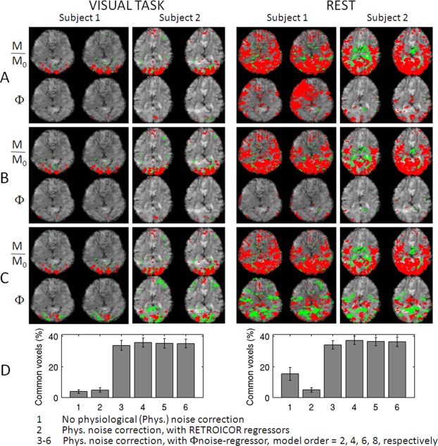
The removal of background low‐frequency phase (Φ) variation increases the sensitivity to BOLD signal changes in phase images and enables the visualization of phase activity maps highly co‐localized to magnitude (M/M₀) activity maps. Magnitude and phase activity maps during visual task (P < 0.05 Bonferroni corrected) and at rest (P < 0.005 Bonferroni corrected, for display purposes only) for two subjects (two slices shown, red/green = positive/negative activity) obtained: (A) without and (B) and (C) with physiological noise correction (temporal drifts were removed in (A–C). The same noise regressors were employed in (B) and (C), with the following exception: the effects related to the phase of respiratory cycle were modeled by (B) four RETROICOR respiratory regressors, and (C) a single Φnoise‐regressor (derived from spatial polynomial fitting of phase images, polynomial order = 4). In (D), we show the percentage (mean ± standard error across subjects) of overlapping voxels between magnitude and phase activity maps relative to the number of voxels in magnitude activity maps (P < 0.05 Bonferroni corrected, for both conditions) with and without physiological noise correction (see legend). In 1, three to six data from eight subjects were pooled, in 2 only six subjects were included because of missing physiological recordings for two subjects. [Color figure can be viewed in the online issue, which is available at http://wileyonlinelibrary.com.]

After physiological noise correction with inclusion of Φnoise‐regressor, similar time‐courses were observed for phase and magnitude signals. For the task data both strongly resembled the stimulation paradigm, suggesting they both primarily reflect BOLD activity (Fig. 4A). The absolute correlation value between magnitude and phase time‐courses (averaged across voxels, and then average ± s.e. across subjects, TE = 31.5 ms) was 0.52 ± 0.02 and 0.42 ± 0.01 during visual task and at rest, respectively, P < 10⁻⁸ (only time‐courses in common positive and negative magnitude and phase activity maps were considered, P < 0.05 Bonferroni corrected).

Figure 4.

BOLD origin of phase (Φ) and magnitude (M/M ₀) signal changes. (A) Averaged phase (black) and magnitude (magenta) time courses in common positive and negative magnitude and phase activity maps (echo time, TE = 31.5 ms, P < 0.05 Bonferroni corrected), for one subject during visual task and at rest (before averaging across voxels, timeseries in negative activity maps were multiplied by −1). The high temporal correlation between phase and magnitude time‐courses indicates the same BOLD origin of phase and magnitude signal changes. For each condition, we plot respectively in (B) and (C) the amplitude of magnitude and phase signal fluctuations versus TE (average ± standard error across subjects) and a linear fit to each data‐set. For each subject, the amplitude of signal fluctuations was measured as the standard deviation of the average time‐course across voxels pertaining to both magnitude and phase activity maps. The increase in amplitude of signal fluctuations with TE was very similar between magnitude and phase data (the correlation between the two was 0.94 ± 0.03 and 0.99 ± 0.00 for the visual task and rest data, respectively, mean ± standard error across eight subjects). [Color figure can be viewed in the online issue, which is available at http://wileyonlinelibrary.com.]

As expected for a BOLD dominated contrast mechanism, fractional magnitude and phase changes increased approximately linearly with TE (Fig. 4B and C). The slope of a linear fit of the amplitude of M/M ₀ signal with TEs (average ± s.e. across subjects) $\Delta R_2^{*}$ of −0.51 ± 0.05 Hz and −0.27 ± 0.02 Hz, yielded respectively, during stimulation and rest.

Estimation of Changes in Fractional Oxygenation from Frequency Shifts in the Sagittal Sinus

For Experiment 1, we inspected more closely Δω/ω ₀ and M/M ₀ during stimulation in the sagittal sinus (Figure 5B, blue arrow, two representative subjects). The strong anti‐correlation (mean r‐value ± standard error across eight subjects = −0.63 ± 0.07, P < 10⁻¹⁶) between the Δω/ω ₀ and M/M ₀ time‐courses (Fig. 5E) confirmed the BOLD origin of Δω/ω ₀ signal fluctuations in the sagittal sinus. In the sagittal sinus, <Δω _A‐B/ω ₀> was (−1.6 ± 0.3) ppb (mean ± standard error across eight subjects); <ΔY _A‐B> computed using Eq. (3) (θ = (14 ± 3)°, mean ± standard error across subjects) was 0.040 ± 0.009 (mean ± standard error across eight subjects); for each subject, θ was measured from the data accounting for the actual oblique slice rotation angle.

Quantitative BOLD Susceptibility Changes

Analysis of the data obtained in Experiment 2 revealed widespread susceptibility changes (Δχ) for all the subjects (see, in Figure 6A, two representative subjects, TE = 31.5 ms). The percentage (mean ± standard error across subjects) of overlapping voxels between Δχ and M/M ₀ activity maps relative to the number of voxels in M/M ₀ activity maps was 25.1 ± 2.5%; the percentage of overlapping voxels between Δω/ω ₀ and M/M ₀ was 35.8 ± 2.6%. The observed quantitative Δχ changes in brain (containing tissue and vessels) are directly related to blood fractional oxygen saturation and blood volume changes and overcome non local effects and the geometry dependence of Δω/ω ₀ signals.

Figure 6.

Quantitative BOLD susceptibility changes. (A) M/M ₀, Δω/ω ₀, and Δχ activity maps during visual task (P < 0.05 Bonferroni corrected) for two subjects participating in Experiment 2 (three slices shown, red/green = positive/negative activity) overlaid on a magnitude EPI image (showed without overlay on the fourth row). The blue arrow indicates the location of large vessels scrutinized in (B). (B) M/M ₀ (green solid line) and Δχ (blue solid line) time‐courses extracted from large vessels shown in (A) [sagittal sinus for subject 1; large vein for subject 2; the sign of Δχ was inverted for display purposes only; Δχ was computed using Eq. (1)]. (C) ≪ΔM _A‐B/M ₀≫ in visual cortex versus <ΔY _A‐B> in the sagittal sinus across subjects (solid line = linear fit). (D) <Δχ _A‐B> and <ΔM _A‐B/M ₀> signal changes (average difference during stimulation with respect to baseline) versus average baseline magnitude values <M ₀> (the sign of <Δχ> was inverted for display purposes only; only voxels showing significant positive M/M ₀ and negative Δχ signal changes were considered, P < 0.05 Bonferroni corrected). Results for subject 1 are displayed. Similar results were obtained for the other subjects. [Color figure can be viewed in the online issue, which is available at http://wileyonlinelibrary.com.]

For instance, for a large vein with θ = 80° (indicated by the blue arrow, in Figure 6A, for subject 2) positive intravascular effects and negative extra‐vascular effects are present in Δω/ω ₀ signals, in agreement with the expected dipolar fields around areas with susceptibility shifts. After deconvolution according to Eq. (1), this dipolar activity pattern in Δω/ω ₀ signals reduces to negative intravascular only effects in Δχ signals. This intravascular decrease in χ signals is caused by increased blood fractional oxygen saturation. The effects for a large vein (sagittal sinus) oriented parallel to B ₀ (measured θ = 0°) are shown in Figure 6A, subject 1. M/M ₀ and Δχ [computed using Eq. (1)] time courses extracted from these two veins (subject 1 and 2, respectively) displayed a significant negative correlation (P < 10⁻³¹, Figure 6B), as expected for increases in blood fractional oxygen saturation. In these two veins (subject 1 and 2, respectively), the increase in fractional oxygen saturation <ΔY _A‐B> was 0.042 and 0.015, as computed from Eq. (4) (calculated values for <Δχ _A‐B> were −3.0 and −1.1 ppb respectively). Corresponding values for <ΔM _A‐B/M ₀> were 5.7 and 6.7%, respectively. At the group level, in the sagittal sinus, <ΔY _A‐B> computed using Eq. (4) was 0.048 ± 0.009 and <Δχ _A‐B> was (−3.5 ± 0.6) ppb (mean ± standard error across six subjects). The intersubject variability in <ΔY _A‐B> in the sagittal sinus correlated (P < 0.05, see Figure 6C) with the intersubject variability in magnitude signal changes (≪ΔM _A‐B/M ₀≫) in the visual cortex (for each subject, ≪ΔM _A‐B/M ₀≫ was computed averaging <ΔM _A‐B/M ₀> across voxels showing positive correlation of M/M ₀ signal changes with the stimulus regressor‐P < 0.05 Bonferroni corrected).

Susceptibility changes were not confined only to the largest vessels, but also appeared to involve the cortex, probably because of BOLD effects in oriented intracortical and pial veins (Fig. 6A). Interestingly, in the visual cortex, the highest absolute <Δχ _A‐B> and <ΔM _A‐B/M ₀> occurred for low values of M ₀ (Fig. 6D). This probably relates to higher blood volume fractions in these regions, because blood $T_2^{*}$ is shorter than tissue $T_2^{*}$ and higher blood volume fractions result in lower M ₀. For instance, according to Eq. (2), a <Δχ _A‐B> = −3.6 ppb is expected for a large vein (for instance a pial vein or a sinus) with Y _A = 0.65, ΔY _A‐B = 0.05, CBV_B = 1, ΔCBV_A‐B = 0, while a <Δχ _A‐B> = −0.18 ppb is expected for few intracortical veins contained in the same voxel with Y _A = 0.75, ΔY _A‐B = 0.10, CBV_B = 0.05, ΔCBV_A‐B = 0.01.

DISCUSSION

In this study we explored the feasibility to use phase signals for the detection of BOLD activity and quantify associated changes in tissue susceptibility related to changes in blood fractional oxygen saturation and in blood volume.

Optimization of fMRI Φ Image Processing

BOLD susceptibility changes in response to activation can be extracted from phase signals by removing confounding effects due to instrumental and physiological sources, which so far have limited effective use of phase signals.

We found that instrumental and physiological noise represented a major source of signal variance in phase signals (about 94% during stimulation), compared to the contribution of BOLD signal fluctuations (about 1%). In contrast, in magnitude data, the contribution of noise sources (variance explained of about 24%) was comparable to that of BOLD signal changes (25% variance explained). This is in line with previous work [Hagberg et al., 2012] showing that noise from physiological and instrumental sources contributes significantly more to the phase than to the magnitude signal instability. Our results also indicate the need of optimized strategies to disentangle tiny BOLD contributions from large signal fluctuations due to noise.

Our optimized preprocessing of phase data was based on a time‐point by time‐point removal of spatial low‐frequency variation, estimated from phase images with a spatial polynomial function. The spatial polynomial fit accounted mainly for slow signal fluctuations over time (signal drifts) and for signal changes related to the phase of the respiratory cycle (Fig. 1, and Table 1). Our slice‐by‐slice approach complements the prospective noise correction performed by real‐time shimming [van Gelderen et al., 2007], which also employs polynomial models of phase variation but on average across the whole brain.

Here, we demonstrated that the MRI signal to noise ratio is adequate to fit low‐spatial‐frequency phase variation by a spatial polynomial function to each time‐point of phase EPI data. We also demonstrated that the resulting time‐course obtained from this fit can be employed on a voxel‐by‐voxel basis as a noise regressor (Φnoise‐regressor) both for phase and for magnitude fMRI data. The effectiveness of the Φnoise‐regressor as a regressor for magnitude data does not depend on the sign of the correlation between phase and magnitude signal changes (the sign is accounted for in the regression). We found (Fig. 2) that the Φnoise‐regressor accounted better (>64% of the variance) for the spatially varying phase effects of respiration in the brain than regressors (<21% of the variance) derived from respiratory recordings [RETROICOR respiratory regressors, Glover et al., 2000]. Its performance was favorable compared to that of the RETROICOR respiratory regressors even for magnitude images. Previous work [Petridou et al., 2009] has shown that although RETROICOR regressors accounted for large‐scale effects induced by respiration in phase signals, they incompletely accounted for physiological noise in phase signals in the gray matter for echo time greater than or equal to 30 ms. The apparently superior performance of the Φnoise‐regressor may be related to the fact that it treats time‐points separately, and thus more generally accommodates a broad variety of noise sources irrespective of their temporal dynamics, including sources that are not cyclic in nature (like respiratory and cardiac cycles). RETROICOR regressors account only for effects related to the phase of respiratory (or cardiac) effects. The ability of RETROICOR regressors to capture such sources is dependent on the model order used, and may be rather limited with the second order model employed in the standard implementation of RETROICOR [Glover et al., 2000] and in the current study. The proposed processing method based on the use of Φnoise‐regressor was also effective in reducing phase noise and unveiling BOLD phase changes for the two data‐sets acquired without real‐time B ₀ shimming. We therefore believe that real‐time B ₀ modulation may not be necessary to detect BOLD phase variations; rather, such variations may be at least partially recovered through the proposed use of Φnoise‐regressor or by any other effective processing method. Finally, we found that Φnoise‐regressor does not remove stimulus related variance, since the stimulus regressor explained a negligible portion of its variance (Table 1). Together, these results demonstrate that the proposed image‐based pre‐processing procedure of phase signals allows one to disentangle instrumental and physiological noise from signals of interest and is advantageous with respect to previously employed methods based on external physiological monitoring.

The results of this work obtained at 7 T may also translate to lower field strength. Although the BOLD related phase change will be proportionally smaller at lower field strength, so will be the major (nonthermal) noise sources; in addition, the thermal noise contribution may be minimized by increasing the voxel size [Triantafyllou et al., 2005]. Thus, depending on the scan conditions, the ability to extract BOLD related phase and frequency changes may not be substantially different at 3 T or even 1.5 T. Nevertheless, some sensitivity loss may occur at low field when considering the partial volume effects that occur when increasing the voxel size.

BOLD Origin of Magnitude and Phase Signal Fluctuations

After noise correction including the subtraction of spatially fitted polynomials, we obtained phase activity maps that substantially (∼40%) overlapped magnitude maps and involved a substantial area of the brain. This extends previous work that showed phase signal changes confined mainly to large sinuses and largest pial veins [Menon, 2002; Nencka and Rowe, 2007]. The distinct spatial distribution of activity in magnitude and phase data may reflect the different contribution arising from “randomly” distributed (e.g., capillary networks) versus oriented (e.g., large veins, pial, and intracortical veins) vessels to magnitude and phase signal changes, respectively.

Similar time‐courses were observed for phase and magnitude signals, indicating the same BOLD origin of phase and magnitude signals changes, namely variation in both blood volume and fractional oxygen saturation. Temperature variations and direct effects of neuronal currents on the B₀ field are therefore unlikely to explain the observed phase signal changes. Moreover, from multiecho magnitude and phase data, we estimated a change in transverse relaxation rate $R_2^{*}$ of −0.51 and −0.27 Hz associated to a frequency shift Δω/ω ₀ of 0.25 and 0.18 ppb during stimulation and at rest respectively. These values are of the same order of magnitude as those reported in the visual cortex during stimulation in previous work [Zhao et al., 2007] on animals at 9.4 T ( $\Delta R_2^{*}$ of −0.87 Hz, and a slope—i.e. angular frequency—of 1.86 radians/s for phase changes with respect to TE, which corresponds to 0.74 ppb).

Finally, our work demonstrated that BOLD changes in phase signals can be detected with comparable sensitivity to those in magnitude signals. This is visible from Figure 4A) (both M/M ₀ and ΔΦ are within the ±5% range around the baseline value), and also comparing (Figure 4B and C) the absolute value of $\Delta R_2^{*}$ (i.e. 0.51 and 0.27 Hz during stimulation and rest, respectively) with the change in angular frequency in the same conditions (equal to 2π·γ _T B ₀·Δω/ω ₀, that is 0.47 and 0.34 radians/s, respectively).

Quantitative BOLD Susceptibility Changes

In previous work, information from fMRI phase signals was used to improve the specificity of BOLD magnitude signal changes, for example to suppress the signal from large vasculature [Menon, 2002], or to increase the sensitivity of BOLD signal changes by performing complex based fMRI analysis [Calhoun et al., 2002; Rowe and Logan, 2004; Lee et al., 2007].

In this work, we investigated the feasibility of computing dynamic BOLD susceptibility changes from phase signal fluctuations; we also investigated the feasibility of estimating quantitative information from BOLD frequency shift and susceptibility maps, namely changes in the blood fractional oxygen saturation in large vessels during stimulation.

We found significant BOLD susceptibility changes Δχ not only inside large vessels, but also in the parenchyma, probably indicating the contribution of oriented pial and intracortical veins. According to our calculations (see Results section), changes in blood fractional oxygen saturation and blood volume in intracortical and pial veins may induce changes in susceptibility ranging from fractions of a ppb to a few ppb. Our data (see also Figure 6B,C,D) demonstrate that high field MRI has adequate sensitivity to detect such small susceptibility variations.

In contrast, blood oxygenation and blood volume changes in capillaries are not expected to be easily detectable in susceptibility images because of their pseudo‐random orientation. Interestingly, previous work [Lee et al., 2010] on phase structural imaging in rats showed a detectable contrast due to intracortical veins; this was not the case for the gray matter containing capillaries.

Computation of Δχ has certain benefits compared to ΔΦ and Δω/ω ₀, since it overcomes their geometry dependence and nonlocal effects. This means that the sign of the observed quantitative Δχ changes in tissue (for instance containing oriented intracortical veins) may directly depend on the counterbalancing effects of blood fractional oxygen saturation and of blood volume changes (and not on the vessels orientation with respect to B ₀). For example, negative Δχ changes in tissue may result from increased blood fractional oxygen saturation in intracortical veins, this effect dominating the counterbalancing effect of increased blood volume changes in the same vessels. Similarly, a shift of this balance could result in positive Δχ changes in tissue. Nevertheless, this suggests that it may be difficult to separate the contribution of fractional oxygen saturation changes from that of blood volume changes to the measured Δχ changes in tissue. Δχ [Eq. (2)] is linearly related both to baseline values and to changes in blood oxygenation and blood volume (four unknown parameters); this is also true for magnitude BOLD signal changes. Untangling these contributions may require separate measurement of baseline blood volume and baseline fractional oxygen saturation, some modeling of the network geometry, and the combined use of magnitude and phase information.

Estimation of Changes in Fractional Oxygenation in Large Veins

In this work, we showed the feasibility of estimating changes in the blood fractional oxygen saturation in large vessels during stimulation. The obtained average change in blood fractional oxygen saturation (<ΔY _A‐B>) in the sagittal sinus and large veins of 0.02–0.05 is close to previous findings obtained with PET imaging [Ito et al., 2005], which report a change in the oxygen extraction fraction (equal to minus the change in fractional oxygen saturation) during motor task with respect to baseline ranging between −0.01 and −0.12, depending on the brain area. Previous MRI work [Haacke et al., 1997] using gradient‐recalled‐echo images and steady state conditions, reported in pial veins a change of fractional oxygen saturation of 0.14 during finger tapping with respect to baseline. Note that the change in blood fractional oxygen saturation in the sagittal sinus and large veins is expected to be smaller than that in the cortex due to downstream dilution from the activation site [Turner, 2002]. For vessels with their axis nearly parallel or perpendicular to B ₀, the estimate of <ΔY _A‐B> from <Δω _A‐B/ω ₀> is robust (<4% error) provided small estimation errors (<10°) in the vessel orientation, but it becomes increasingly dependent on the vessel orientation with respect to B ₀ when it is close to the magic angle (54.74°). Computation of susceptibility changes instead overcomes the orientation dependence and local effects of <Δω _A‐B/ω ₀>, though the measurement constrains the acquisition to coronal/sagittal slices (or to a thick axial slab, with a good z‐coverage) and requires the use of procedures to compute susceptibility from frequency shifts [Shmueli et al., 2009; Wharton et al., 2010] that are not fully developed yet.

The method employed here to estimate the changes in the blood fractional oxygen saturation from standard gradient‐echo EPI images complements previous work measuring baseline values in large vessels by means of gradient‐recalled‐echo structural images [Jain et al., 2010; Fan et al., 2012]. It is also an improvement in terms of temporal resolution with regard to previous work measuring changes in blood fractional oxygen saturation in large vessels by means of gradient‐recalled‐echo images under steady state conditions [Haacke et al., 1997]. Nevertheless, our estimation of blood fractional oxygen saturation is restricted to large vessels “containing” the imaging voxel (for instance the sagittal sinus), and therefore is limited by the spatial resolution. The employed spatial resolution (2.5 mm isotropic) in this work is below the achievable resolution with cutting edge technology (around 1 mm in plane, or slightly below), and future work with higher spatial resolution EPIs should investigate if this method of estimating blood fractional oxygen saturation changes can be applied more locally (for example to pial veins).

CONCLUSIONS

Widespread BOLD‐related phase changes, frequency shifts and susceptibility changes could be detected at 7 T with sensitivity comparable to that of magnitude signals by the use of optimized preprocessing to remove unwanted phase signal fluctuations. The measured susceptibility changes do not seem to be confined to venous sinuses, but rather indicate widespread involvement of pial and intracortical veins. BOLD susceptibility changes obtained from phase images are related to average quantitative susceptibility changes due to variation in blood volume and fractional oxygen saturation, and might provide complementary information to BOLD relaxation rate changes obtained from magnitude images.

We also demonstrated the feasibility of estimating the functional change in blood fractional oxygen saturation in large veins during task performance by analyzing BOLD frequency shift and susceptibility maps computed from the phase signal in gradient‐echo fMRI. With activation, fractional oxygen saturation in the sagittal sinus and large veins was found to increase by about 0.02–0.05, consistent with estimates reported in literature.

REFERENCES

- Bianciardi M, van Gelderen P, Duyn J (2012): Estimation of functional changes in blood oxygenation level in large veins from BOLD frequency shift and susceptibility maps. Proc. Int. Soc. Mag. Reson. Med, Melbourne, Australia, Abstract no. 2201. [Google Scholar]
- Bianciardi M, van Gelderen P, Duyn J (2011a): BOLD frequency shifts in human fMRI at 7 T. ISMRM Scientific Workshop on Ultra‐High Field Systems & Applications: 7 T & Beyond: Progress, Pitfalls & Potential, Lake Louise, Alberta, Canada.
- Bianciardi M, Fukunaga M, van Gelderen P, de Zwart JA, Duyn JH (2011b): Negative BOLD‐fMRI signals in large cerebral veins. J Cereb Blood Flow Metab 31:401–412. [DOI] [PMC free article] [PubMed] [Google Scholar]
- Bianciardi M, Fukunaga M, van Gelderen P, Horovitz SG, de Zwart JA, Shmueli K, Duyn JH (2009): Sources of functional magnetic resonance imaging signal fluctuations in the human brain at rest: A 7 T study. Magn Reson Imaging 27:1019–1029. [DOI] [PMC free article] [PubMed] [Google Scholar]
- Birn RM, Diamond JB, Smith MA, Bandettini PA (2006): Separating respiratory‐variation‐related fluctuations from neuronal‐activity‐related fluctuations in fMRI. Neuroimage 31:1536–1548. [DOI] [PubMed] [Google Scholar]
- Calhoun VD, Adali T, Pearlson GD, van Zijl PC, Pekar JJ (2002): Independent component analysis of fMRI data in the complex domain. Magn Reson Med 48:180–192. [DOI] [PubMed] [Google Scholar]
- Duyn JH, van Gelderen P, Li TQ, de Zwart JA, Koretsky AP, Fukunaga M (2007): High‐field MRI of brain cortical substructure based on signal phase. Proc Natl Acad Sci USA 104:11796–11801. [DOI] [PMC free article] [PubMed] [Google Scholar]
- Fan AP, Benner T, Bolar DS, Rosen BR, Adalsteinsson E (2012): Phase‐based regional oxygen metabolism (PROM) using MRI. Magn Reson Med 67:669–678. [DOI] [PMC free article] [PubMed] [Google Scholar]
- Glover GH, Li TQ, Ress D (2000): Image‐based method for retrospective correction of physiological motion effects in fMRI: RETROICOR. Magn Reson Med 44:162–167. [DOI] [PubMed] [Google Scholar]
- Guyton AC, Hall JE (2000). Red blood cells, anemia, and polycythemia In: Guyton AC, Hall JE, editors. Textbook of Medical Physiology. Philadelphia: Saunders; pp 382–391. [Google Scholar]
- Haacke EM, Lai S, Reichenbach JR, Kuppusamy K, Hoogenraad FGC, Takeichi H, Lin W (1997): In vivo measurement of blood oxygen saturation using magnetic resonance imaging: A direct validation of the blood oxygen level‐dependent concept in functional brain imaging. Hum Brain Mapp 5:341–346. [DOI] [PubMed] [Google Scholar]
- Hagberg GE, Bianciardi M, Brainovich V, Cassara AM, Maraviglia B (2012): Phase stability in fMRI time series: Effect of noise regression, off‐resonance correction and spatial filtering techniques. Neuroimage 59:3748–3761. [DOI] [PubMed] [Google Scholar]
- Hahn AD, Nencka AS, Rowe DB (2009): Improving robustness and reliability of phase‐sensitive fMRI analysis using temporal off‐resonance alignment of single‐echo timeseries (TOAST). Neuroimage 44:742–752. [DOI] [PMC free article] [PubMed] [Google Scholar]
- He X, Yablonskiy DA (2007): Quantitative BOLD: Mapping of human cerebral deoxygenated blood volume and oxygen extraction fraction: Default state. Magn Reson Med 57:115–126. [DOI] [PMC free article] [PubMed] [Google Scholar]
- Ito H, Ibaraki M, Kanno I, Fukuda H, Miura S (2005): Changes in cerebral blood flow and cerebral oxygen metabolism during neural activation measured by positron emission tomography: Comparison with blood oxygenation level‐dependent contrast measured by functional magnetic resonance imaging. J Cereb Blood Flow Metab 25:371–377. [DOI] [PubMed] [Google Scholar]
- Jain V, Langham MC, Wehrli FW (2010): MRI estimation of global brain oxygen consumption rate. J Cereb Blood Flow Metab 30:1598–1607. [DOI] [PMC free article] [PubMed] [Google Scholar]
- Lee J, Hirano Y, Fukunaga M, Silva AC, Duyn JH (2010): On the contribution of deoxy‐hemoglobin to MRI gray–white matter phase contrast at high field. Neuroimage 49:193–198. [DOI] [PMC free article] [PubMed] [Google Scholar]
- Lee J, Shahram M, Schwartzman A, Pauly JM (2007): Complex data analysis in high‐resolution SSFP fMRI. Magn Reson Med 57:905–917. [DOI] [PubMed] [Google Scholar]
- Menon RS (2002): Postacquisition suppression of large‐vessel BOLD signals in high‐resolution fMRI. Magn Reson Med 47:1–9. [DOI] [PubMed] [Google Scholar]
- Nencka AS, Rowe DB (2007): Reducing the unwanted draining vein BOLD contribution in fMRI with statistical post‐processing methods. Neuroimage 37:177–188. [DOI] [PubMed] [Google Scholar]
- Ogawa S, Menon RS, Tank DW, Kim SG, Merkle H, Ellermann JM, Ugurbil K (1993): Functional brain mapping by blood oxygenation level‐dependent contrast magnetic resonance imaging. A comparison of signal characteristics with a biophysical model. Biophys J 64:803–812. [DOI] [PMC free article] [PubMed] [Google Scholar]
- Petridou N, Schafer A, Gowland P, Bowtell R (2009): Phase vs. magnitude information in functional magnetic resonance imaging time series: Toward understanding the noise. Magn Reson Imaging 27:1046–1057. [DOI] [PubMed] [Google Scholar]
- Rooney WD, Johnson G, Li X, Cohen ER, Kim SG, Ugurbil K, Springer CS (2007): Magnetic field and tissue dependencies of human brain longitudinal 1H2O relaxation in vivo. Magn Reson Med 57:308–18. [DOI] [PubMed] [Google Scholar]
- Rowe DB, Logan BR (2004): A complex way to compute fMRI activation. Neuroimage 23:1078–1092. [DOI] [PubMed] [Google Scholar]
- Shmueli K, de Zwart JA, van Gelderen P, Li TQ, Dodd SJ, Duyn JH (2009): Magnetic susceptibility mapping of brain tissue in vivo using MRI phase data. Magn Reson Med 62:1510–1522. [DOI] [PMC free article] [PubMed] [Google Scholar]
- Shmueli K, van Gelderen P, de Zwart JA, Horovitz SG, Fukunaga M, Jansma JM, Duyn JH (2007): Low‐frequency fluctuations in the cardiac rate as a source of variance in the resting‐state fMRI BOLD signal. Neuroimage 38:306–320. [DOI] [PMC free article] [PubMed] [Google Scholar]
- Smith AM, Lewis BK, Ruttimann UE, Ye FQ, Sinnwell TM, Yang Y, Duyn JH, Frank JA (1999): Investigation of low frequency drift in fMRI signal. Neuroimage 9:526–533. [DOI] [PubMed] [Google Scholar]
- Triantafyllou C, Hoge RD, Krueger G, Wiggins CJ, Potthast A, Wiggins GC, Wald LL (2005): Comparison of physiological noise at 1.5 T, 3 T and 7 T and optimization of fMRI acquisition parameters. Neuroimage 26:243–250. [DOI] [PubMed] [Google Scholar]
- Turner R (2002): How much cortex can a vein drain? Downstream dilution of activation‐related cerebral blood oxygenation changes. Neuroimage 16:1062–1067. [DOI] [PubMed] [Google Scholar]
- van Gelderen P, de Zwart JA, Starewicz P, Hinks RS, Duyn JH (2007): Real‐time shimming to compensate for respiration‐induced B0 fluctuations. Magn Reson Med 57:362–368. [DOI] [PubMed] [Google Scholar]
- Weisskoff RM, Kiihne S (1992): MRI susceptometry: Image‐based measurement of absolute susceptibility of MR contrast agents and human blood. Magn Reson Med 24:375–383. [DOI] [PubMed] [Google Scholar]
- Wharton S, Schafer A, Bowtell R (2010): Susceptibility mapping in the human brain using threshold‐based k‐space division. Magn Reson Med 63:1292–1304. [DOI] [PubMed] [Google Scholar]
- Yan L, Zhuo Y, Ye Y, Xie SX, An J, Aguirre GK, Wang J (2009): Physiological origin of low‐frequency drift in blood oxygen level dependent (BOLD) functional magnetic resonance imaging (fMRI). Magn Reson Med 61:819–827. [DOI] [PubMed] [Google Scholar]
- Zhao F, Jin T, Wang P, Hu X, Kim SG (2007): Sources of phase changes in BOLD and CBV‐weighted fMRI. Magn Reson Med 57:520–527. [DOI] [PubMed] [Google Scholar]