

Abstract
Purpose
Owing to variability in vascular dynamics across cerebral cortex, blood-oxygenation-level-dependent (BOLD) spatial and temporal characteristics should vary as a function of cortical-depth. Here, the positive response, initial dip (ID), and post-stimulus-undershoot (PSU) of the BOLD response in human visual cortex are investigated as a function of cortical depth and stimulus duration at 7T.
Methods
Gradient-echo echo-planar-imaging BOLD fMRI with high spatial and temporal resolution was performed in 7 healthy volunteers and measurements of the ID, PSU and positive BOLD response were made as a function of cortical depth and stimulus duration (0.5s–8s). Exploratory analyses were applied to understand whether functional mapping could be achieved using the ID, rather than positive, BOLD signal characteristics.
Results
The ID was largest in outer cortical layers, consistent with previously reported upstream propagation of vasodilation along the diving arterioles in animals. The positive BOLD signal and PSU showed different relationships across the cortical depth with respect to stimulus duration.
Conclusion
The ID and PSU were measured in humans at 7T and exhibited similar trends to those recently reported in animals. Furthermore, while evidence is provided for the ID being a potentially useful feature for better understanding BOLD signal dynamics, such as laminar neurovascular coupling, functional mapping based on the ID is extremely difficult.
Keywords: BOLD, fMRI, cortical depth, hemodynamic response, initial dip, undershoot, vasodilation
Introduction
Functional magnetic resonance imaging (fMRI), which most commonly exploits the blood-oxygenation-level-dependent (BOLD) contrast (1), does not require exogenous contrast agents and therefore is an invaluable tool for obtaining repeated functional measurements, assessing longitudinal changes in brain function, and for probing pathophysiological mechanisms in clinical scenarios where contrast agents may be contraindicated. As a result, BOLD fMRI has emerged as the most important tool for assessing brain function with a wide variety of clinical, pharmacological and neuroscience applications to date (2–4).
However, the BOLD fMRI signal is only an indirect marker of neuronal activity, arising from complex neurochemical, metabolic, and hemodynamic modulations that occur concurrent to both ongoing and stimulus-evoked neuronal activity. Specifically, in stimulus-evoked experiments, BOLD contrast arises owing to a greater increase in cerebral blood flow (CBF) relative to cerebral blood volume (CBV) and the cerebral metabolic rate of oxygen (CMRO2), leading to an increase in diamagnetic oxyhemoglobin relative to paramagnetic deoxyhemoglobin in capillaries and veins (1,5,6). While much progress has been made in understanding the hemodynamic and metabolic contributions to BOLD contrast, important gaps remain in our ability to improve localization of BOLD contrast to neuronal activity relative to draining veins. These gaps significantly hinder BOLD interpretability in many applications, as substantial variability in BOLD responses exists between even healthy individuals, partly accounting for why BOLD data remain largely qualitative in nature. Understanding the physiological sources of this variability and the spatial and temporal inaccuracies of the BOLD signal are fundamental to using BOLD as a tool for identifying quantitative differences in brain function between individuals and conditions, and for gauging functional response to disease and treatment.
The BOLD hemodynamic response function (HRF) has been reported to be comprised of (i) a transient reduction in signal (initial dip, ID), followed by (ii) a positive increase in signal, concluding with (iii) a signal reduction below baseline (post-stimulus undershoot, PSU) (7,8). However, the reproducibility and spatial heterogeneity of both the ID and PSU have been debated (9–13). It is also well-known that the positive BOLD signal arises due to the reduction of venous deoxyhemoglobin leading to local magnetic field disturbances (a T2(*) effect) in and around capillaries and veins, the extent of which may or may not be well-localized to tissue. Positive BOLD signal changes thus reflect CBF changes that carry convolved contributions from neuronal activation (neurovascular coupling) and from non-specific passive blood draining. Non-specific passive blood draining is especially prominent near the cortical surface and is caused by blood pooling from blood vessels of upstream activation sites (i.e. deeper cortical layers). It is difficult to isolate, and therefore remove, the contribution from passive blood draining in the positive response, as positive BOLD signal is derived from many physiological effects, with few direct observables.
To better localize functional activation to regions of metabolic activation there has been variable interest in using negative temporal features of the evoked BOLD response. The ID may arise from a faster increase in CMRO2 relative to CBF (9–12,14) ,and the PSU has been debated to arise from delayed vascular compliance (7,15), persisting elevated CMRO2 (10,16), and/or reduced CBF (17,18). Importantly, these negative HRF components may reflect more specific metabolic and/or hemodynamic properties than positive HRF components, possibly increasing spatial specificity to activation. Owing to the hypothesized increased spatial sensitivity of these features, the coarse spatial resolution (3–5 mm) and large intravascular BOLD contributions at 1.5 T-3.0 T, mechanistic studies of negative BOLD responses have provided conflicting data.
Very recently, 7 T fMRI performed at high spatial and temporal resolution has been used to reveal information concerning the temporal evolution of the positive BOLD response across the cortical depth in human brain, suggesting that relationships of neurovascular coupling vary across cortical layers (19). Slightly earlier studies in cat visual cortex at high spatial resolution demonstrated that BOLD responses are largest near the cortical surface, whereas both CBF and CBV increase most in deeper cortical layers (20). These findings, combined with the hypothesized origins of the ID and PSU suggest that these negative BOLD responses should additionally be cortical depth dependent. Indeed recent work combining BOLD fMRI and two-photon microscopy in rat somatosensory cortex has provided evidence for the ID being largest in surface cortical layers, a finding that has been hypothesized to arise from upstream propagation of vasodilation toward the cortical surface along diving arterioles, while CMRO2 increases near-simultaneously in all layers (21). Early fMRI work at 7 T demonstrated the detectability of the ID at high spatial resolution at this field strength (12), however no work has focused on characterizing the cortical depth dependence of the ID or the PSU in humans.
As signal-to-noise ratio (SNR), BOLD contrast-to-noise ratio (CNR) and extravascular BOLD sensitivity all increase with increasing static magnetic field strength (22,23), 7 T MRI carries potential for enabling increased spatial and temporal resolution that can better elucidate the origins of the ID and PSU. However, as mentioned above comparatively few 7 T BOLD methodological studies focus on the ID and PSU, with the majority of studies addressing positive aspects of the HRF (19,24–26). Therefore, it was the aim of this study to measure spatial and temporal features of the ID and PSU in addition to the positive BOLD signal as a function of cortical depth and stimulus duration at 7 T and at increased temporal and spatial resolution. Results are intended to provide insight into the spatial and temporal characteristics of the ID and PSU in humans, and to demonstrate how observed trends are consistent with recent work in anaesthetized animals (21,27).
Methods
Experiment
Volunteers (n=7; age=32+/−15 yrs; 3F/4M) provided informed, written consent in accordance with the local ethics committee and were scanned at 7 T (Philips Medical Systems) using a transmit head coil and a 32-channel receive coil. Prior to fMRI acquisition, a field map (B0) was acquired and third order image-based shimming was performed over the visual cortex. Next, coronal, gradient echo (GRE) EPI BOLD images (TR/TE=600/25 ms; 1.3×1.3×1.3 mm3; field-of-view (FOV)=140×140 mm2; slices=6, slice gap=0 mm; SENSE factor=2.2; flip angle = 55º) were positioned over the visual cortex, as identified by a high resolution T2*-weighted (T2*w) anatomical scan (3D multishot GRE-EPI, TR/TE=105/20 ms; 0.5×0.5×0.5 mm3; FOV=188×188×30 mm3; SENSE factor=2; flip angle=20º) applied with the same scan geometry (slice position and angulation) as the BOLD scans (28). BOLD data were acquired for five different visual (blue/yellow 8 Hz flashing checkerboard) paradigms, each with separate stimulus duration/repetition blocks: 0.5s/16, 1s/8, 2s/5, 4s/5 and 8s/5, and all with a constant inter-stimulus baseline period of 16s plus 16s of initial baseline scanning to allow signal to reach steady state. Note that the functional duty cycle (baseline duration / stimulus duration) varied from 32 (0.5s stimulus) to 2 (8s stimulus). For the duty cycle of 2, it is possible that signal will not have returned to baseline in some subjects and voxels. Therefore, the 8s stimulus data were included as exploratory and the main study conclusions were based on 0.5s-4s stimulus duration data. The number of repetition blocks was varied between stimulus duration scans to maintain a similar CNR in all experiments.
Analysis
BOLD data were corrected for motion, baseline drift and re-gridded to the T2*w anatomical scan using standard algorithms (29,30). The cortical surface was manually delineated on the high resolution T2*w scan for slices where the calcarine sulcus was clearly visible. In regions where the sulcus was visible, the shortest distance (i.e. the Euclidian distance in three dimensions) to the cortical surface was computed. Next, the voxels were binned according to their cortical distance to give three depth ROIs for subsequent cortical depth analysis: 0–1 mm (Region 1, R1: superficial gray matter), 1–2 mm (Region 2, R2: intermediate gray matter), and 2–3 mm (Region 3, R3: deep gray matter). To ensure no voxels were included which were not activated, we multiplied the depth ROIs by a localizer activation mask, obtained from a standard GLM analysis of the 4s stimulus data (z-stat threshold=2.3 and cluster P-value threshold=0.05) using FSL FEAT, (30). The z-stat threshold was kept relatively low for strong visual stimulation so as to reduce the mask from being biased by subtle fluctuations that may be dependent on the ID. In other words, the activation mask reflected a relatively non-specific mask that included voxels near both large and small vessels. The final ROI mask was subsequently co-registered to the high resolution T2*w scan and smoothed with a 2.6 mm Gaussian kernel. The time-series data were interpolated to 100 ms to facilitate correct block-averaging for all stimulus durations.
The statistical aims of this study were to measure, as a function of cortical depth and stimulus duration, (i) the magnitude of the positive BOLD response, and (ii) the magnitude of the ID. A more exploratory aim was to assess (iii) the magnitude of the PSU in relation to the other BOLD response components (positive response and ID). The positive BOLD response was recorded as the mean of voxel time points during or after cessation of stimulus as defined by the points between when the signal reached a plateau (or peak in the case of the stimulus = 0.5s time course) and before it began to decline toward baseline. As the HRF is slow (2–5s) with respect to the measurement TR (600ms), we found that this procedure provided the most accurate representation of the positive BOLD response. The ID was calculated as the minimum signal in the time course prior to the beginning of the onset of the positive response and after the signal had returned to baseline. As the ID is expected to be small and possibly within the noise level of the signal fluctuations, two additional analyses were considered. First, we calculated the standard deviation of the baseline signal (final 5s in each baseline block) in each subject and recorded whether the ID was more than one standard deviation beyond the baseline signal fluctuation. Second, z-statistics for the ID statistical map were calculated by computing the mean of the period of 1.3–3.0 s (from t=0s) from the average BOLD response (estimated using a deconvolution approach (conjugate-gradient method (31)) divided by the standard deviation of the first baseline signal (16s). This method was preferred over a conventional GLM approach to reduce the error of misidentifying the ID as a post stimulus undershoot signal. This analysis step essentially evaluates the potential utility of using the ID time course as a target for functional mapping. Our hypothesis was that the ID would be largest in the outer cortical layer (R1) relative to the deep cortical layer (R3), which could be attributed to a temporal mismatch in the onset of the CBF, CBV and CMRO2 responses following stimulation. To understand how the size of the ID may vary with such a temporal mismatch, we applied existing models of BOLD contrast with different temporal offsets (0–2s) to simulate the evolution of the ID under these conditions (5,32).
The PSU was quantified as the minimum signal below baseline following stimulus cessation and before the signal returned to baseline. Finally, while the ID occurs transiently prior to a positive response and therefore should not be influenced by the magnitude of the positive response, the PSU may be influenced by the magnitude of the positive response. Therefore, we additionally normalized the PSU by the magnitude of the positive response to understand to what extent the post-stimulus changes are being driven by cortical depth and stimulus duration versus simply the size of the positive response.
To assess significance between cortical layers, a paired Student’s t-test (one tail) was applied, whereby for each subject the desired measurement for each stimulus block was compared for each cortical depth ROI with Pitalic>0.05 required for significance. Descriptive statistics, including means, standard deviations, and ranges for continuous parameters, as well as percent and frequency for categorical parameters, were evaluated.
Results
Figure 1 shows the results of the simulation, whereby representative pure gray matter time courses for CBF, CBV and CMRO2 are shown (left) relative to the corresponding calculated evoked BOLD response (right) for (A) no delay between onset of the hemo-metabolic parameters, (B) a 0.5s delay in the onset of CBF and CBV relative to CMRO2, and (C) a 1s shift in the onset of the CBF and CBV changes relative to CMRO2. Note that as the shift in time becomes larger for these parameters, the ID also grows in magnitude. The ID is not apparent for no temporal mismatch, but grows to −0.003, −0.0117, and −0.0291 for temporal shifts of 0.5s, 1s, and 2s, respectively. Therefore, for very small temporal differences between CBF/CBV and CMRO2 changes of bold>1s, the ID magnitude is <1%, whereas this grows substantially as the mismatch grows beyond 1s. Note that besides a timing mismatch also the magnitude of the CMRO2 changes will modulate the ID magnitude.
Figure 1.

(Left) Cerebral blood flow (CBF), cerebral blood volume (CBV), and cerebral metabolic rate of oxygen consumption (CMRO2) changes for (A) no temporal mismatch between CBF/CBV and CMRO2, (B) a 0.5s temporal mismatch in onset times, and (C) a 1s temporal mismatch in onset times. (Right) The corresponding simulated BOLD responses, which display how the initial dip increases in magnitude for larger temporal mismatches between CBF/CBV and CMRO2.
Figure 2 shows the cortical depth ROIs used in analysis for all seven subjects in three separate planes, separately for the anatomical images and for the anatomical images with the masks overlaid.
Figure 2.

Region of interest (ROI) maps for each subject. Blue = Region 1 (R1: superficial); Red = Region 2 (R2: intermediate); and Green = Region 3 (R3: deep).
Figure 3A–B shows, for a single-subject, block-averaged time course for the 8s stimulus duration, which provides a measure of the noise level on a single-subject level. It can be seen that both the ID and the positive response vary with cortical depth, with the ID and positive response being largest in the most superficial layer (R1) and decreasing for deeper cortical layers (R2 and R3). Additionally, it can be seen that the signal appears to return to baseline by the conclusion of the 16s baseline period. This response time is faster than that simulated in Figure 1 owing to the simulation reflecting a pure cortical voxel with no effects from partial volume contributions. Figure 3C–F also shows the mean, block-averaged time courses for all subjects, demonstrating a similar trend in the positive response as was observed in the single-subject time course (Figure 3A–B). The ID in the subject averaged time-course however is much less apparent, which is likely due to inter-subject variability in timing and magnitude of the BOLD signal evolution. The ID was observed for all stimulus durations though at decreased magnitude. Figure 4A shows the BOLD responses from a single subject across the cortical depth including a 1.5s pre-stimulus period for the 4s stimulus duration (data for all other subjects can be found in Supplementary Figure 1). It can be seen that the CNR was sufficient for assessing the ID across the cortical depth when averaging over each cortical depth ROI. Figure 4B shows that the ID map is rather noisy and not estimated reliably throughout the V1 gray matter on a voxel basis. This illustrates that it is challenging when using the ID as a mapping tool for functional activation, especially for high spatial resolution fMRI studies where the SNR is relatively low.
Figure 3.

(A) Block-averaged time course and (B) magnified first 4s from a volunteer (stimulus duration= 8s) for the three different regions of interest shown in Figure 2. Note that the initial dip is observed to be largest in R1 and smallest in R3. Blue = Region 1 (R1: superficial); Red = Region 2 (R2: intermediate); and Green = Region 3 (R3: deep). The mean (n=7) block-averaged time courses for (C) Region 1, (D) Region 2, and (E) Region 3. (F) A magnification of the first 4s (shown here for stimulus duration = 8s) shows a slightly larger mean ID in R1 relative to R2 and R3.
Figure 4.
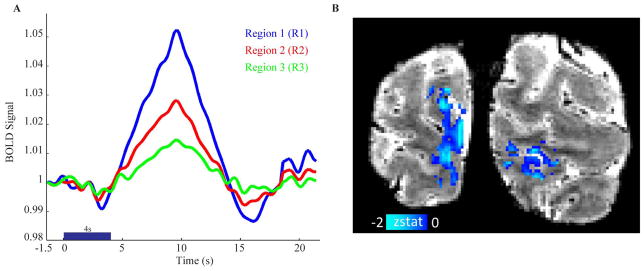
(A) BOLD response across the cortical depth showing a 1.5s pre-stimulus period and the subsequent initial dip (ID) for each cortical depth region for the 4s stimulus duration from a volunteer (Blue = Region 1 (R1: superficial); Red = Region 2 (R2: intermediate); and Green = Region 3 (R3: deep)). The BOLD responses shown were estimated using a non-parametric deconvolution (conjugate-gradient method,(31)) of the signal with the stimulus design train. (B) ID map (z-statistic) for the same subject and stimulus duration. Using the ID as a mapping tool is challenging for high spatial resolution fMRI studies as the ID map is rather noisy and not estimated reliably throughout the gray matter on a voxel basis. However, when averaging over regions as shown in panel (A), the ID could prove to be useful for studying BOLD signal characteristics in relation to, for instance, laminar neurovascular coupling mechanisms.
Table 1 shows positive responses for all subjects, stimulus durations and cortical depths, as well as the magnitude of the ID for all subjects, stimulus durations and cortical depths.
Table 1. (Above) Positive signal changes.
The top row denotes the stimulus duration and the second row the region analyzed for Region 1 (R1: most superficial); Region 2 (R2; intermediate); and Region 3 (R3; deep). (Below) Initial dip values. The top row denotes the stimulus duration and the second row the region analyzed.
| 0.5s | 0.5s | 0.5s | 1s | 1s | 1s | 2s | 2s | 2s | 4s | 4s | 4s | 8s | 8s | 8s | |
|---|---|---|---|---|---|---|---|---|---|---|---|---|---|---|---|
| Subject | R1 | R2 | R3 | R1 | R2 | R3 | R1 | R2 | R3 | R1 | R2 | R3 | R1 | R2 | R3 |
| 1 | 0.008 | 0.007 | 0.006 | 0.018 | 0.017 | 0.012 | 0.022 | 0.020 | 0.015 | 0.034 | 0.022 | 0.019 | 0.041 | 0.034 | 0.025 |
| 2 | 0.025 | 0.016 | 0.009 | 0.027 | 0.019 | 0.012 | 0.039 | 0.024 | 0.016 | 0.045 | 0.026 | 0.018 | 0.052 | 0.033 | 0.021 |
| 3 | 0.012 | 0.007 | 0.005 | 0.024 | 0.017 | 0.014 | 0.014 | 0.010 | 0.007 | 0.027 | 0.017 | 0.014 | 0.041 | 0.028 | 0.023 |
| 4 | 0.028 | 0.016 | 0.012 | 0.034 | 0.021 | 0.016 | 0.048 | 0.030 | 0.026 | 0.062 | 0.037 | 0.033 | 0.079 | 0.047 | 0.035 |
| 5 | 0.028 | 0.017 | 0.009 | 0.028 | 0.017 | 0.010 | 0.028 | 0.019 | 0.012 | 0.046 | 0.025 | 0.013 | 0.047 | 0.028 | 0.015 |
| 6 | 0.030 | 0.020 | 0.016 | 0.045 | 0.036 | 0.027 | 0.037 | 0.035 | 0.030 | 0.032 | 0.026 | 0.016 | 0.085 | 0.056 | 0.044 |
| 7 | 0.015 | 0.008 | 0.006 | 0.022 | 0.014 | 0.011 | 0.024 | 0.015 | 0.012 | 0.032 | 0.020 | 0.014 | 0.051 | 0.029 | 0.022 |
| Mean | 0.021 | 0.013 | 0.009 | 0.028 | 0.020 | 0.014 | 0.030 | 0.022 | 0.017 | 0.040 | 0.025 | 0.018 | 0.056 | 0.036 | 0.026 |
| STD | 0.009 | 0.005 | 0.004 | 0.009 | 0.007 | 0.006 | 0.012 | 0.009 | 0.008 | 0.012 | 0.006 | 0.007 | 0.018 | 0.011 | 0.010 |
| 0.5s | 0.5s | 0.5s | 1s | 1s | 1s | 2s | 2s | 2s | 4s | 4s | 4s | 8s | 8s | 8s | |
|---|---|---|---|---|---|---|---|---|---|---|---|---|---|---|---|
| Subject | R1 | R2 | R3 | R1 | R2 | R3 | R1 | R2 | R3 | R1 | R2 | R3 | R1 | R2 | R3 |
| 1 | −0.0013 | −0.0021 | −0.0003 | −0.0032 | −0.0004 | −0.0005 | −0.0022 | −0.0033 | −0.0034 | −0.0008 | −0.0018 | −0.0008 | −0.0085 | −0.0098 | −0.0072 |
| 2 | 0.0000 | −0.0001 | −0.0011 | −0.0048 | −0.0017 | 0.0000 | −0.0028 | −0.0018 | −0.0002 | −0.0021 | −0.0026 | −0.0016 | 0.0000 | 0.0000 | −0.0008 |
| 3 | −0.0010 | −0.0008 | −0.0002 | −0.0010 | −0.0001 | −0.0004 | −0.0001 | −0.0001 | 0.0000 | −0.0009 | −0.0009 | −0.0015 | −0.0007 | −0.0005 | −0.0009 |
| 4 | −0.0003 | −0.0004 | −0.0007 | −0.0028 | −0.0017 | −0.0003 | −0.0003 | −0.0002 | −0.0002 | −0.0002 | −0.0001 | −0.0005 | −0.0002 | −0.0001 | −0.0002 |
| 5 | −0.0022 | −0.0011 | −0.0007 | −0.0003 | −0.0002 | 0.0000 | −0.0009 | −0.0001 | −0.0011 | −0.0094 | −0.0062 | −0.0046 | −0.0038 | −0.0021 | −0.0019 |
| 6 | 0.0000 | 0.0000 | 0.0000 | −0.0006 | −0.0003 | −0.0005 | −0.0039 | −0.0037 | 0.0000 | 0.0000 | 0.0000 | 0.0000 | −0.0042 | −0.0021 | −0.0009 |
| 7 | −0.0008 | −0.0008 | −0.0006 | −0.0025 | −0.0004 | −0.0010 | −0.0006 | −0.0003 | −0.0001 | −0.0040 | −0.0027 | −0.0034 | −0.0038 | −0.0019 | −0.0015 |
| Mean | −0.0008 | −0.0008 | −0.0005 | −0.0021 | −0.0007 | −0.0004 | −0.0016 | −0.0013 | −0.0007 | −0.0025 | −0.0021 | −0.0018 | −0.0030 | −0.0024 | −0.0019 |
| STD | 0.0008 | 0.0007 | 0.0004 | 0.0016 | 0.0007 | 0.0003 | 0.0014 | 0.0016 | 0.0012 | 0.0033 | 0.0021 | 0.0016 | 0.0030 | 0.0034 | 0.0024 |
Figure 5 shows the dependence of the positive and ID responses with cortical depth and stimulus duration. As can be seen, the positive responses increase with decreasing cortical depth and increasing stimulus duration (Figure 5A). While these two phenomena have been reported separately in previous work (19), here we have looked at the combined effect. Differences were found in the observed relationship between the BOLD response and the stimulus duration with respect to cortical depth. The slope of the line describing this relationship was largest in the outer cortical layer (slope=0.45 %BOLD/s) and decreasing in the intermediate (slope=0.27 %BOLD/s) and deep (slope=0.2 %BOLD/s) cortical layers. Differences between these slopes were all significant at P<0.05. For very short stimulus duration (0.5–1 s), the relationship between the positive BOLD response and the stimulus duration appears to become nonlinear, confirming earlier reports (33,34). In Figure 5B, the magnitude of the ID is plotted against the stimulus duration. For short stimulus durations (0.5–2s), the ID was smallest, yet increased for the longer stimulus durations and did not vary significantly between stimulus duration 4s and 8s. While the size of the ID did vary between these regions, the presence or absence of an ID did not vary significantly between regions analyzed (i.e., if the ID was observed, it was generally observed in all regions, albeit with different magnitudes). Figure 5C shows a boxplot of the ID values, which incorporates all data points (stimulus durations) at each cortical depth region. A significant difference (P<0.05) is found between each cortical layer, with the ID being observed to be largest in the most superficial layer and decreasing in magnitude in deeper layers.
Figure 5.

(A) The mean positive BOLD signal changes (n=7) and (B) mean initial dip (ID) values vs. stimulus duration. The positive BOLD signal changes increase linearly with stimulus duration, with this trend being steepest in R1. The ID is small for short stimulus durations 0.5s-2s, but larger and independent of stimulus duration for longer stimulus durations (4s-8s). Blue = Region 1 (R1: superficial); Red = Region 2 (R2: intermediate); and Green = Region 3 (R3: deep). (C) A boxplot demonstrating the decreasing magnitude of the ID with increasing cortical depth. The plot incorporates all data points (all stimulus durations). The central line is the median, the edges of the box are the 25th and 75th percentiles, and the whiskers extend to the most extreme data points.
Figure 6 shows the PSU values both before (Figure 6A) and after (Figure 6B) normalization by the positive BOLD response. The PSU was difficult to detect for stimulus duration <2 s, but then increases in size for longer stimulus durations (2s – 8s). Therefore, additional PSU analysis focused on the 2s, 4s, and 8s stimulus durations. Figure 6C and 6D show boxplots of the PSU values, respectively before and after normalization, incorporating all data points averaged over stimulus durations 2s – 8s at each cortical depth region. Although not significant at the level of P = 0.05 for all cortical depths, we did observe a trend of the PSU magnitude with cortical-depth for stimulus durations >2s, both before and after normalization with the positive BOLD response though in opposite directions. Before normalization, the trend shows the largest PSU in superficial cortical regions (R1) whereas after normalization the largest PSU seems most strong in the deeper cortical regions (R3). Lastly, we did not find a significant relation or dependency between the PSU and the ID magnitude. Magnitude of the PSU are presented in Table 2.
Figure 6.

Mean post-stimulus undershoot (PSU) signal change (n=7) versus stimulus duration and cortical depth before (A) and after (B) normalizing by the maximum of the positive BOLD response. The PSU was difficult to detect for stimulus durations <2s, but then increases in size for longer stimulus durations (2s – 8s). Error bars denote the standard error of the mean (shown in one direction for clarity). (C) and (D) boxplots (all data points of stimulus durations 2s – 8s and all subjects) demonstrating the cortical depth dependence of the PSU before and after normalizing by the positive BOLD response respectively. Although not significant at the level of P= 0.05, a trend is observed of the PSU with cortical depth where the largest undershoot is found in the superficial cortical layers (R1). This trend reverses after normalization by the positive response as the largest undershoot is found in the deeper cortical layers (R3) after normalization. The central line is the median, the edges of the box are the 25th and 75th percentiles, the whiskers extend to data not considered outliers, and the red crosses indicate outliers (more than two standard deviations beyond the mean).
Table 2.
(Above) Maximum undershoot signal changes.The top row denotes the stimulus duration and the second row the region analyzed for Region 1 (R1: most superficial); Region 2 (R2; intermediate); and Region 3 (R3; deep). (Below) Maximum undershoot signal changes normalized by maximum positive BOLD response. The top row denotes the stimulus duration and the second row the region analyzed.
| 0.5s | 0.5s | 0.5s | 1s | 1s | 1s | 2s | 2s | 2s | 4s | 4s | 4s | 8s | 8s | 8s | |
|---|---|---|---|---|---|---|---|---|---|---|---|---|---|---|---|
| Subject | R1 | R2 | R3 | R1 | R2 | R3 | R1 | R2 | R3 | R1 | R2 | R3 | R1 | R2 | R3 |
| 1 | 0.0002 | −0.0005 | 0.0002 | −0.0017 | 0.0009 | −0.0009 | −0.004 | −0.0021 | −0.0014 | −0.0093 | −0.0058 | −0.0057 | −0.0033 | −0.0052 | −0.0054 |
| 2 | 0.0047 | 0.0023 | −0.0005 | −0.0009 | 0.0016 | 0.0021 | −0.0016 | −0.0036 | −0.0020 | −0.0069 | −0.0062 | −0.0023 | −0.0065 | −0.0056 | −0.0046 |
| 3 | −0.0029 | −0.0026 | −0.0028 | −0.003 | −0.0016 | −0.0013 | −0.021 | −0.0165 | −0.0124 | −0.0015 | −0.002 | −0.001 | −0.0101 | −0.0066 | −0.0049 |
| 4 | 0.0045 | 0.0019 | 0.0000 | −0.0063 | −0.0035 | −0.003 | −0.0011 | −0.0009 | −0.0002 | −0.0067 | −0.0056 | −0.0017 | 0.0006 | −0.0006 | −0.0019 |
| 5 | 0.0001 | 0.0009 | 0.0005 | 0.0028 | 0.0014 | 0.0022 | −0.0007 | 0.0009 | 0.0018 | −0.013 | −0.0079 | −0.0039 | −0.0135 | −0.0084 | −0.0041 |
| 6 | 0.0025 | 0.0017 | 0.0019 | −0.0006 | −0.0008 | −0.0004 | −0.0020 | −0.0015 | −0.0030 | −0.0046 | −0.0064 | −0.0077 | −0.004 | −0.0034 | −0.0054 |
| 7 | 0.0006 | −0.0004 | 0.0002 | −0.0014 | −0.0008 | −0.0001 | 0.0017 | 0.0028 | 0.0013 | −0.0101 | −0.007 | −0.0074 | −0.0062 | −0.0057 | −0.0041 |
| Mean | 0.0014 | 0.0005 | −0.0001 | −0.0016 | −0.0004 | −0.0002 | −0.0041 | −0.0030 | −0.0023 | −0.0074 | −0.0058 | −0.0042 | −0.0061 | −0.0051 | −0.0043 |
| STD | 0.0027 | 0.0017 | 0.0014 | 0.0027 | 0.0018 | 0.0019 | 0.0076 | 0.0063 | 0.0048 | 0.0038 | 0.0019 | 0.0027 | 0.0046 | 0.0025 | 0.0012 |
| 0.5s | 0.5s | 0.5s | 1s | 1s | 1s | 2s | 2s | 2s | 4s | 4s | 4s | 8s | 8s | 8s | |
|---|---|---|---|---|---|---|---|---|---|---|---|---|---|---|---|
| Subject | R1 | R2 | R3 | R1 | R2 | R3 | R1 | R2 | R3 | R1 | R2 | R3 | R1 | R2 | R3 |
| 1 | 0.0250 | −0.0714 | 0.0333 | −0.0944 | 0.0529 | −0.0750 | −0.1818 | −0.1050 | −0.0933 | −0.2735 | −0.2636 | −0.3000 | −0.0805 | −0.1529 | −0.2160 |
| 2 | 0.1880 | 0.1437 | −0.0556 | −0.0333 | 0.0842 | 0.1750 | −0.0410 | −0.1500 | −0.1250 | −0.1533 | −0.2385 | −0.1278 | −0.1250 | −0.1697 | −0.2190 |
| 3 | −0.2417 | −0.3714 | −0.5600 | −0.1250 | −0.0941 | −0.0929 | −1.5000 | −1.6500 | −1.7714 | −0.0556 | −0.1176 | −0.0714 | −0.2463 | −0.2357 | −0.2130 |
| 4 | 0.1607 | 0.1188 | 0.0000 | −0.1853 | −0.1667 | −0.1875 | −0.0229 | −0.0300 | −0.0077 | −0.1081 | −0.1514 | −0.0515 | 0.0076 | −0.0128 | −0.0543 |
| 5 | 0.0036 | 0.0529 | 0.0556 | 0.1000 | 0.0824 | 0.2200 | −0.0250 | 0.0474 | 0.1500 | −0.2826 | −0.3160 | −0.3000 | −0.2872 | −0.3000 | −0.2733 |
| 6 | 0.0833 | 0.0850 | 0.1188 | −0.0133 | −0.0222 | −0.0148 | −0.0541 | −0.0429 | −0.1000 | −0.1438 | −0.2462 | −0.4813 | −0.0471 | −0.0607 | −0.1227 |
| 7 | 0.0400 | −0.0500 | 0.0333 | −0.0636 | −0.0571 | −0.0091 | 0.0708 | 0.1867 | 0.1083 | −0.3156 | −0.3500 | −0.5286 | −0.1216 | −0.1966 | −0.1864 |
| Mean | 0.0370 | −0.0132 | −0.0535 | −0.0593 | −0.0172 | 0.0022 | −0.2506 | −0.2491 | −0.2627 | −0.1904 | −0.2405 | −0.2658 | −0.1286 | −0.1612 | −0.1835 |
| STD | 0.1409 | 0.1775 | 0.2295 | 0.0909 | 0.0957 | 0.1465 | 0.5559 | 0.6274 | 0.6737 | 0.0997 | 0.0830 | 0.1917 | 0.1054 | 0.0986 | 0.0726 |
Discussion
The major findings from this study are (i) for a stimulus duration of 0.5s–8s, the positive BOLD response increases with stimulus duration most steeply in outer cortical layers, and (ii) the ID is largest in outer cortical layers, decreases in magnitude with increasing cortical depth, and increases in magnitude with stimulus duration. These findings generally confirm that the behavior of the ID is similar in humans as has recently been reported in anesthetized animals (21). A supplementary finding was that the magnitude of the PSU shows a trend with cortical depth at the spatial resolution afforded in this study, the sign of which depends on whether the PSU is normalized by the positive BOLD response magnitude. However, several more novel findings were also observed.
Positive BOLD signal findings
The finding of the positive BOLD response decreasing with cortical depth and decreasing stimulus duration is in-line with previous studies in humans that have reported effects of venous pooling in the outer cortical layers (venous blood volume largest near cortical surface) albeit using a single stimulus duration (19,35). This leads to the conclusion that the deeper cortical layers which have a smaller relative fraction of venous CBV may be more sensitive markers of functional activation, however these regions also have reduced sensitivity owing to the smaller magnitude signal change here. This notion is also in agreement with previous animal studies investigating the positive BOLD and/or CBV characteristics across the cortical depth (4,20,21,36–41). Also, we found that the deep cortical layers have faster onset times than the middle and superficial cortical layers (Figure 3B). These findings are in line with recent human fMRI studies on the BOLD response shape (19,42), where a gradual increase in onset time was found with decreasing cortical depth. This seems in contrast with an earlier report by Silva and Koretsky that showed faster onset times for the middle layers in rats (36). Our observed faster onset time in R3 (deep gray matter) is likely due to averaging of several cortical layers within a voxel, where R3 probably contains layer IV (middle layer) and layers V–VI (deep layer) which reduces the ability to resolve the differences observed by Silva and Koretsky in rats (36). Additionally, it can be seen from Figure 5 that the intercept to the linear fit of the positive signal change to the stimulus duration is non-zero in all cortical regions. This finding suggests that the linearity measured here may be unique to intermediate-to-long stimulus durations, yet for very short stimulus durations (<1s) neurovascular coupling relationships may shift to a different regime with a much greater slope, or alternatively exponential behavior. Physiologically, this would be consistent with a large increase in CBF relative to a much smaller increase in CMRO2 or CBV. This may not be surprising as the metabolic demands of such a short stimulus may be small, and furthermore much of the hemodynamic resources required for this sort of response could be derived from changes in capillary flow dynamics (43). Testing of this hypothesis is not possible with the current data, however previous work that employed a range of very short stimulus durations (down to 5ms and 0.33μs in human and rat studies respectively (41,44)), indeed revealed much greater slopes for short stimulus durations (<1s). The finding of a greater slope in the outer cortical layers with stimulus duration can likely be explained as a passive hemodynamic phenomenon, i.e. increased blood pooling in downstream vessels, which would be largest in the outer cortical layers. A recent study by Hirano et al. in rats revealed very similar findings; the outer cortical layers (I–III) showed the most steep slopes of the BOLD signal magnitude versus stimulus duration (41). Moreover, using additional CBF and CBV measurements they demonstrate that for increasing stimulus duration the BOLD response becomes more contaminated by blood pooling in downstream vascular compartments.
Initial dip BOLD findings
Many studies have tried to identify the physiological origin of the ID, primarily using BOLD fMRI and optical data. From BOLD fMRI work on the ID, it is commonly thought that the ID is caused by initial increases in deoxyhemoglobin (elevated CMRO2) upon neuronal activation followed by a delayed CBF response (8,9,12,21,44). Conversely, Sirotin et al. recently observed, using intrinsic optical imaging data from primates, that the ID could be due to early increases in CBV without any initial change in deoxyhemoglobin (CMRO2) (45). Early increases in CBV can also produce a negative BOLD signal, especially at high magnetic field strength (7 T) where one is dominated by extravascular BOLD signals (11). This notion was first suggested by Buxton et al. and incorporated into the empirical Balloon model (7). The original Balloon model also suggests that vasodilation is substantial in veins, whereas optical imaging studies have shown larger effects in arterioles. Explaining the discrepancies between these optical and fMRI results is challenging as the field-of-view can be substantially different between techniques. Optical imaging is heavily dominated by superficial cortical signals (these regions are also most dense with arterioles), whereas fMRI can resolve cortical depth-dependent BOLD responses (19,21,36,42). It is likely that the exact origin of the observed ID of the BOLD response is dependent on a mixture of factors that could vary across the cortical layers. It has been hypothesized that the ID of the BOLD response could be used for improved localization of functional activation. Previous optical and fMRI studies have demonstrated that the initial dip might be able to reveal columnar like structures in cats (46,47), and may have a narrower spatial point spread function than the positive hyperemic BOLD response (45,48). We find however that the feasibility for the ID as a mapping tool in humans, even at 7 T, remains very difficult.
The findings in this study demonstrate for the first time in humans at 7 T that the ID is dependent on cortical depth, with the largest response occurring near the cortical surface. This finding is consistent with recent a study by Tian et al. in anaesthetized rats, combing two-photon microscopy and BOLD fMRI (21). Their two-photon microscopy data showed an upstream propagation of vasodilation along penetrating arterioles toward the cortical surface, where the CBF response is substantially delayed thus causing the largest CBF/CMRO2 timing mismatch (21). This notion concurs with their BOLD fMRI findings; the largest positive BOLD response delay and initial dip magnitude was found in the upper cortical layers. We show that this finding can similarly be observed in humans at 7 T. The larger IDs observed in the outer cortical regions correspond to the location of largest venous pooling effects in the positive response, and are in the close vicinity of the larger pial draining veins. This might explain the observed variability in detecting the ID at lower spatial and temporal resolutions and lower field strengths where the BOLD contrast is dominated by intravascular BOLD signals (49). Investigation on the effect of a lower spatial resolution (~ 3mm) on our data revealed indeed a reduced heterogeneity and detectability of the ID (see Supplementary Figure 2). A possible approach to reduce these nonspecific signals in the BOLD response would be by using crusher gradients or spin-echo BOLD (42). This however will come at a price in SNR. Interestingly, the larger ID in the outer cortical gray mater may also be caused by increased local CMRO2 (neuronal activation) due to the blue-yellow stimulus. Olman et al. showed that a colored stimulus preferentially activates the outer gray matter (the so-called parvocellular pathway) in the visual cortex as opposed to a changing luminance stimulus (50). Our setup was not specifically designed to confirm these findings by using the ID, however future experiments could elaborate on the potential of the ID to resolve laminar neurovascular coupling mechanisms. Local information on CMRO2 would be ideal to investigate the ID characteristics and laminar neurovascular coupling mechanisms, however independent measures of CMRO2 using MRI is currently extremely difficult to achieve. Our findings suggest that in deep cortical layers the ID is very small and may not be detectable in the majority of functional imaging experiments with insufficient SNR. It should be mentioned that in contrast to the study by Tian et al, other studies on the rat somatosensory cortex have not or scarcely been able to detect the initial dip (36,51,52). This could, however, be caused by methodological issues such as different voxel size, sampling time, field strength or anesthesia. Work using laser Doppler flowmetry and O2 microelectrodes in rat somatosensory cortex have detected transient decreases in partial pressure of tissue O2 (pO2) before an increase in CBF and an overshoot of tissue pO2 (53). These direct observations indicate early CMRO2 changes, uncoupled of the CBF response, thus allowing the existence of an ID in the corresponding BOLD response. Ultimately, using the ID as a mapping tool to specifically demarcate regions of metabolic/neuronal activity may be difficult. However, negative BOLD responses, such as the ID, might provide useful insight in neurovascular coupling mechanisms across cortical lamina, as recently suggested in a study on primates (40).
Post-stimulus undershoot BOLD findings
The PSU changes we observed are consistent with high-resolution studies from the animal literature. In cat visual cortex, the absolute PSU was observed to be largest in the upper cortical layers (20). In a separate study at high-spatial resolution in cat visual cortex, it was shown, as we found, that the BOLD PSU is present in both surface and deeper cortical regions (39,54). Interestingly, our observed trend with cortical depth seems to reverse after normalization by the positive BOLD response (now largest undershoot is found in the deeper cortical regions, which was also observed in cat visual cortex (20). We hypothesize that normalizing by the positive response will partially correct for blood draining effects at the cortical surface, and could indicate that the deeper cortical regions exhibit a larger PSU. Blood containing increased deoxyhemoglobin content (during the period of the PSU) is eventually collected in surface cortical regions from multiple upstream sites (i.e. from deeper cortical regions), similarly as during the positive BOLD response. Normalizing by the positive BOLD response for each cortical depth region would partially correct for this draining nuisance, therefore evincing more local neurovascular and metabolic processes. A large PSU in deeper cortical regions could be explained by the higher density of neurons located in the deeper cortical layers (higher metabolic demand, (55)) and would support the metabolic hypothesis concerning the physiological origin of the PSU; increased CMRO2 changes following stimulation and uncoupling of CBF/CMRO2 (56,57). Recent work in rats by Herman et al. (4) using calibrated fMRI have shown evidence for higher CMRO2 increases in deeper cortical regions, whereas the cortical gradient of changes in CBV and CBF showed a reversed profile (albeit to a lesser extent for the CBF changes). It should be noted however that Herman et al. recorded the cortical profiles of CMRO2, CBV, and CBF during the period of the positive BOLD response upon an excitatory task. Interestingly, recent work in monkeys (40) and humans (58) observed that the cortical CBV profile reverses between an excitatory and inhibitory task (thus during a positive and negative BOLD response, respectively). These studies suggest that positive and negative BOLD responses may comprise different neurovascular and metabolic coupling mechanisms, which may also apply to the PSU (40,58). Lastly, our findings can also be explained by the CBF reducing below baseline during the PSU. This notion cannot be excluded as CBF measurements were not obtained. Owing to the difficulty of obtaining CBF and CBV measurements in humans currently at 7 T, our study reports only on BOLD changes as a function of cortical depth. However, our data demonstrate that similar BOLD findings to those reported in animals at very high field can also be found in humans using 7 T fMRI. At high field, ideally one would like to perform high spatial and temporal resolution multi-modal measurements of hemodynamics combined with calibrated fMRI or spectroscopy for incorporating metabolic information as has been performed in animals (4,59) or electrophysiology for including measures of neuronal activity (60,61). Advances towards the multi-modal assessment at 7 T of hemodynamics and neuronal activity have been demonstrated in humans at 7 T (58,62), and future work and improvements in this field will deepen our understanding on neurovascular coupling mechanisms.
Limitations
Several limitations of this study should be considered. First, while our experiments were performed at much higher spatial and temporal resolution (spatial resolution = 1.3 mm; temporal resolution = 0.6 s)) than is typically performed at 1.5 T-3.0 T (spatial resolution = 3–5 mm; temporal resolution = 2–3s), it is still not possible to make quantitative claims regarding different cortical layers as at most 3 voxels were lined up along the cortical depth. However, spatial differences smaller than the image resolution (cortical depth bin size = 1 mm versus voxel size = 1.3 mm) can be resolved because of the convoluted shape of the human cortex and partial-volume effects when averaging many data points on isotropic voxel size data. This increases the effective spatial resolution for this type of analysis (63). Nonetheless, the findings must still be interpreted in terms largely of outer, middle and deeper cortical regions. Second, even with relatively high spatial and temporal resolution, the ID was difficult to detect beyond the noise level of the time course in some volunteers and experiments. Third, the baseline time of 16s may not be sufficient for the signal to return to baseline for long stimuli ≥8s. While this was not a complication on average (see Figures 3–4), nor in the shorter stimulus 0.5s-4s experiments, caution should be exercised when interpreting the post-stimulus return time for this stimulus duration. The reason for this baseline choice was so that all experiments could be performed within a one hour scan session, however a separate study whereby stimulus duration is held constant, and a longer baseline period is allowed would be of interest for interrogating post-stimulus changes following long stimuli. Fourth, as with other high resolution fMRI studies, volume coverage was limited in our study. Therefore, inflow effects could complicate the patterns observed here. However, our findings are consistent with other animal studies using both BOLD and non-MRI techniques, and therefore we believe that this is not an overwhelming complication.
Conclusion
We have demonstrated that in addition to positive aspects of the BOLD response, negative BOLD responses such as the initial dip and post-stimulus undershoot demonstrate substantial and significant heterogeneity across the human cortical depth. These findings provide some understanding why these temporal features of the BOLD effect are variably reported at conventional field strengths and spatial resolutions and extend recently reported cortical depth dependence studies in animals to humans. Feasibility of the initial dip as a robust mapping tool for neuronal activation remains unresolved, however it might provide usefulness in gaining more insight in cortical depth dependent neurovascular coupling mechanisms.
Supplementary Material
Acknowledgments
We thank the following sources of support: The Netherlands Society for Scientific Research, and NIH/NINDS 1R01NS07882801.
Footnotes
Declaration of Conflict of Interest
The authors have no conflict of interest to declare with regards to the content of this work.
References
- 1.Kim S, Ogawa S. Biophysical and physiological origins of blood oxygenation level-dependent fMRI signals. J Cereb Blood Flow Metab. 2012:1–19. doi: 10.1038/jcbfm.2012.23. [DOI] [PMC free article] [PubMed] [Google Scholar]
- 2.Jezzard P, Buxton RB. The clinical potential of functional magnetic resonance imaging. J Magn Reson Imaging. 2006;23:787–793. doi: 10.1002/jmri.20581. [DOI] [PubMed] [Google Scholar]
- 3.Kim SG, Duong TQ. Mapping cortical columnar structures using fMRI. Physiol Behav. 2002;77:641–644. doi: 10.1016/S0031-9384(02)00901-0. [DOI] [PubMed] [Google Scholar]
- 4.Herman P, Sanganahalli BG, Blumenfeld H, Rothman DL, Hyder F. Quantitative basis for neuroimaging of cortical laminae with calibrated functional MRI. Proc Natl Acad Sci U S A. 2013;110:15115–15120. doi: 10.1073/pnas.1307154110. [DOI] [PMC free article] [PubMed] [Google Scholar]
- 5.Buxton RB, Uludağ K, Dubowitz DJ, Liu TT, Uluda? K. Modeling the hemodynamic response to brain activation. Neuroimage. 2004;23 (Suppl 1):S220–S233. doi: 10.1016/j.neuroimage.2004.07.013. [DOI] [PubMed] [Google Scholar]
- 6.Van Zijl PC, Eleff SM, Ulatowski JA, Oja JM, Ulug AM, Traystman RJ, Kauppinen RA. Quantitative assessment of blood flow, blood volume and blood oxygenation effects in functional magnetic resonance imaging. Nat Med. 1998;4:159–167. doi: 10.1038/nm0298-159. [DOI] [PubMed] [Google Scholar]
- 7.Buxton RB, Wong EC, Frank LR. Dynamics of blood flow and oxygenation changes during brain activation: the balloon model. Magn Reson Med. 1998;39:855–864. doi: 10.1002/mrm.1910390602. [DOI] [PubMed] [Google Scholar]
- 8.Hu X, Yacoub E. The story of the initial dip in fMRI. Neuroimage. 2012;62:1103–1108. doi: 10.1016/j.neuroimage.2012.03.005. [DOI] [PMC free article] [PubMed] [Google Scholar]
- 9.Buxton RB. The elusive initial dip. Neuroimage. 2001;13:953–8. doi: 10.1006/nimg.2001.0814. [DOI] [PubMed] [Google Scholar]
- 10.Donahue MJ, Stevens RD, de Boorder M, Pekar JJ, Hendrikse J, van Zijl PCM, De Boorder M, Van Zijl PCM. Hemodynamic changes after visual stimulation and breath holding provide evidence for an uncoupling of cerebral blood flow and volume from oxygen metabolism. J Cereb Blood Flow Metab. 2009;29:176–185. doi: 10.1038/jcbfm.2008.109. [DOI] [PMC free article] [PubMed] [Google Scholar]
- 11.Uludag K. To dip or not to dip: reconciling optical imaging and fMRI data. Proc Natl Acad Sci U S A. 2010;107:E23. doi: 10.1073/pnas.0914194107. author reply E24. [DOI] [PMC free article] [PubMed] [Google Scholar]
- 12.Yacoub E, Shmuel A, Pfeuffer J, Van De Moortele PF, Adriany G, Ugurbil K, Hu X. Investigation of the initial dip in fMRI at 7 Tesla. NMR Biomed. 2001;14:408–412. doi: 10.1002/nbm.715. [DOI] [PubMed] [Google Scholar]
- 13.van Zijl P, Hua J, Lu H. The BOLD post-stimulus undershoot, one of the most debated issues in fMRI. Neuroimage. 2012:1–11. doi: 10.1016/j.neuroimage.2012.01.029. [DOI] [PMC free article] [PubMed] [Google Scholar]
- 14.Hyder F, Rothman DLD. Quantitative fMRI and oxidative neuroenergetics. Neuroimage. 2012;62:985–994. doi: 10.1016/j.neuroimage.2012.04.027. [DOI] [PMC free article] [PubMed] [Google Scholar]
- 15.Mandeville JB, Marota JJ, Ayata C, Moskowitz MA, Weisskoff RM, Rosen BR. MRI measurement of the temporal evolution of relative CMRO(2) during rat forepaw stimulation. Magn Reson Med. 1999;42:944–51. doi: 10.1002/(sici)1522-2594(199911)42:5<944::aid-mrm15>3.0.co;2-w. [DOI] [PubMed] [Google Scholar]
- 16.Lu H, Golay X, Pekar JJ, Van Zijl PCM. Sustained poststimulus elevation in cerebral oxygen utilization after vascular recovery. J Cereb Blood Flow Metab. 2004;24:764–70. doi: 10.1097/01.WCB.0000124322.60992.5C. [DOI] [PubMed] [Google Scholar]
- 17.Friston KJ, Mechelli A, Turner R, Price CJ. Nonlinear responses in fMRI: the Balloon model, Volterra kernels, and other hemodynamics. Neuroimage. 2000;12:466–477. doi: 10.1006/nimg.2000.0630. [DOI] [PubMed] [Google Scholar]
- 18.Hoge RD, Atkinson J, Gill B, Crelier GR, Marrett S, Pike GB. Stimulus-dependent BOLD and perfusion dynamics in human V1. Neuroimage. 1999;9:573–85. doi: 10.1006/nimg.1999.0443. [DOI] [PubMed] [Google Scholar]
- 19.Siero JCW, Petridou N, Hoogduin H, Luijten PR, Ramsey NF. Cortical depth-dependent temporal dynamics of the BOLD response in the human brain. J Cereb Blood Flow Metab. 2011;31:1999–2008. doi: 10.1038/jcbfm.2011.57. [DOI] [PMC free article] [PubMed] [Google Scholar]
- 20.Jin T, Kim S-G. Cortical layer-dependent dynamic blood oxygenation, cerebral blood flow and cerebral blood volume responses during visual stimulation. Neuroimage. 2008;43:1–9. doi: 10.1016/j.neuroimage.2008.06.029. [DOI] [PMC free article] [PubMed] [Google Scholar]
- 21.Tian P, Teng IIC, May LDL, et al. Cortical depth-specific microvascular dilation underlies laminar differences in blood oxygenation level-dependent functional MRI signal. Proc Natl Acad Sci U S A. 2010;107:15246–51. doi: 10.1073/pnas.1006735107. [DOI] [PMC free article] [PubMed] [Google Scholar]
- 22.Donahue MJ, Hoogduin H, van Zijl PCM, Jezzard P, Luijten PR, Hendrikse J, Van Zijl PCM. Blood oxygenation level-dependent (BOLD) total and extravascular signal changes and ΔR2* in human visual cortex at 1.5, 3.0 and 7.0 T. NMR Biomed. 2011;24:25–34. doi: 10.1002/nbm.1552. [DOI] [PubMed] [Google Scholar]
- 23.Van Der Zwaag W, Francis S, Head K. fMRI at 1.5, 3 and 7 T: characterising BOLD signal changes. Neuroimage. 2009;47:1425–1434. doi: 10.1016/j.neuroimage.2009.05.015. [DOI] [PubMed] [Google Scholar]
- 24.Duong TQ, Yacoub E, Adriany G, Hu X, Ugurbil K, Vaughan JT, Merkle H, Kim S-G. High-resolution, spin-echo BOLD, and CBF fMRI at 4 and 7 T. Magn Reson Med. 2002;48:589–93. doi: 10.1002/mrm.10252. [DOI] [PubMed] [Google Scholar]
- 25.Donahue MJ, Hoogduin H, Smith SM, Siero JCW, Chappell M, Petridou N, Jezzard P, Luijten PR, Hendrikse J. Spontaneous blood oxygenation level-dependent fMRI signal is modulated by behavioral state and correlates with evoked response in sensorimotor cortex: a 7.-T fMRI study. Hum Brain Mapp. 2012;33:511–22. doi: 10.1002/hbm.21228. [DOI] [PMC free article] [PubMed] [Google Scholar]
- 26.Shmuel A, Yacoub E, Chaimow D, Logothetis NK, Ugurbil K. Spatio-temporal point-spread function of fMRI signal in human gray matter at 7 Tesla. Neuroimage. 2007;35:539–552. doi: 10.1016/j.neuroimage.2006.12.030. [DOI] [PMC free article] [PubMed] [Google Scholar]
- 27.Chen BR, Bouchard MBM, McCaslin AFHA, Burgess SA, Hillman EMC. High-speed vascular dynamics of the hemodynamic response. Neuroimage. 2011;54:1021–1030. doi: 10.1016/j.neuroimage.2010.09.036. [DOI] [PMC free article] [PubMed] [Google Scholar]
- 28.Zwanenburg JJMM, Versluis MJ, Luijten PR, Petridou N. Fast high resolution whole brain T2* weighted imaging using echo planar imaging at 7T. Neuroimage. 2011;56:1902–7. doi: 10.1016/j.neuroimage.2011.03.046. [DOI] [PubMed] [Google Scholar]
- 29.Jenkinson M, Smith S. A global optimisation method for robust affine registration of brain images. Med Image Anal. 2001;5:143–156. doi: 10.1016/s1361-8415(01)00036-6. [DOI] [PubMed] [Google Scholar]
- 30.Jenkinson M, Beckmann CF, Behrens TEJ, Woolrich MW, Smith SM. FSL. Neuroimage. 2012;62:782–790. doi: 10.1016/j.neuroimage.2011.09.015. [DOI] [PubMed] [Google Scholar]
- 31.Ari N, Yen Y. Extraction of the Hemodynamic Response in Randomized Event-Related Functional MRI. Proceedings? 23rd Annual Conference? IEEE/EMBS; Oct.25–28, 2001; Istanbul, TURKEY. 2001. pp. 0–4. [Google Scholar]
- 32.Sotero RC, Trujillo-Barreto NJ. Modelling the role of excitatory and inhibitory neuronal activity in the generation of the BOLD signal. Neuroimage. 2007;35:149–165. doi: 10.1016/j.neuroimage.2006.10.027. [DOI] [PubMed] [Google Scholar]
- 33.Miller KL, Luh W-M, Liu TT, Martinez A, Obata T, Wong EC, Frank LR, Buxton RB. Nonlinear temporal dynamics of the cerebral blood flow response. Hum Brain Mapp. 2001;13:1–12. doi: 10.1002/hbm.1020. [DOI] [PMC free article] [PubMed] [Google Scholar]
- 34.Soltysik DA, Peck KK, White KD, Crosson B, Briggs RW. Comparison of hemodynamic response nonlinearity across primary cortical areas. Neuroimage. 2004;22:1117–1127. doi: 10.1016/j.neuroimage.2004.03.024. [DOI] [PubMed] [Google Scholar]
- 35.Petridou N, Italiaander M, van de Bank BL, Siero JCW, Luijten PR, Klomp DWJ, Van De Bank BL. Pushing the limits of high-resolution functional MRI using a simple high-density multi-element coil design. NMR Biomed. 2013;26:65–73. doi: 10.1002/nbm.2820. [DOI] [PubMed] [Google Scholar]
- 36.Silva AC, Koretsky AP. Laminar specificity of functional MRI onset times during somatosensory stimulation in rat. Proc Natl Acad Sci U S A. 2002;99:15182–15187. doi: 10.1073/pnas.222561899. [DOI] [PMC free article] [PubMed] [Google Scholar]
- 37.Shen Q, Ren H, Duong TQ. CBF, BOLD, CBV, and CMRO(2) fMRI signal temporal dynamics at 500-msec resolution. J Magn Reson Imaging. 2008;27:599–606. doi: 10.1002/jmri.21203. [DOI] [PMC free article] [PubMed] [Google Scholar]
- 38.Kim T, Kim S-G. Temporal dynamics and spatial specificity of arterial and venous blood volume changes during visual stimulation: implication for BOLD quantification. J Cereb Blood Flow Metab. 2011;31:1211–22. doi: 10.1038/jcbfm.2010.226. [DOI] [PMC free article] [PubMed] [Google Scholar]
- 39.Zhao F, Jin T, Wang P, Kim S-G. Improved spatial localization of post-stimulus BOLD undershoot relative to positive BOLD. Neuroimage. 2007;34:1084–92. doi: 10.1016/j.neuroimage.2006.10.016. [DOI] [PMC free article] [PubMed] [Google Scholar]
- 40.Goense J, Merkle H, Logothetis NK. High-Resolution fMRI Reveals Laminar Differences in Neurovascular Coupling between Positive and Negative BOLD Responses. Neuron. 2012;76:629–639. doi: 10.1016/j.neuron.2012.09.019. S0896-6273(12)00854-9 [pii] [DOI] [PMC free article] [PubMed] [Google Scholar]
- 41.Hirano Y, Stefanovic B, Silva A. Spatiotemporal evolution of the functional magnetic resonance imaging response to ultrashort stimuli. J Neurosci. 2011;31:1440–1447. doi: 10.1523/JNEUROSCI.3986-10.2011. [DOI] [PMC free article] [PubMed] [Google Scholar]
- 42.Siero JCW, Ramsey NF, Hoogduin H, Klomp DWJ, Luijten PR, Petridou N. BOLD specificity and dynamics evaluated in humans at 7 T: comparing gradient-echo and spin-echo hemodynamic responses. PLoS One. 2013;8:e54560. doi: 10.1371/journal.pone.0054560. [DOI] [PMC free article] [PubMed] [Google Scholar]
- 43.Jespersen SN, ⊘stergaard L. The roles of cerebral blood flow, capillary transit time heterogeneity, and oxygen tension in brain oxygenation and metabolism. J Cereb Blood Flow Metab. 2012;32:264–77. doi: 10.1038/jcbfm.2011.153. [DOI] [PMC free article] [PubMed] [Google Scholar]
- 44.Yeşilyurt B, Uğurbil K, Uludağ K. Dynamics and nonlinearities of the BOLD response at very short stimulus durations. Magn Reson Imaging. 2008;26:853–862. doi: 10.1016/j.mri.2008.01.008. [DOI] [PubMed] [Google Scholar]
- 45.Sirotin YB, Hillman EMC, Bordier C, Das A. Spatiotemporal precision and hemodynamic mechanism of optical point spreads in alert primates. Proc Natl Acad Sci U S A. 2009;106:18390–5. doi: 10.1073/pnas.0905509106. [DOI] [PMC free article] [PubMed] [Google Scholar]
- 46.Duong TQ, Kim DS, Uğurbil K, Kim SG. Spatiotemporal dynamics of the BOLD fMRI signals: toward mapping submillimeter cortical columns using the early negative response. Magn Reson Med. 2000;44:231–42. doi: 10.1002/1522-2594(200008)44:2<231::aid-mrm10>3.0.co;2-t. [DOI] [PubMed] [Google Scholar]
- 47.Kim DS, Duong TQ, Kim SG. High-resolution mapping of iso-orientation columns by fMRI. Nat Neurosci. 2000;3:164–9. doi: 10.1038/72109. [DOI] [PubMed] [Google Scholar]
- 48.Watanabe M, Bartels A, Macke JH, Murayama Y, Logothetis NK. Temporal Jitter of the BOLD Signal Reveals a Reliable Initial Dip and Improved Spatial Resolution. 2013. pp. 2146–2150. [DOI] [PubMed] [Google Scholar]
- 49.Uludag K, Moëller-Bierl B, Ugurbil K. An integrative model for neuronal activity-induced signal changes for gradient and spin echo functional imaging. Neuroimage. 2009;48:150–165. doi: 10.1016/j.neuroimage.2009.05.051. [DOI] [PubMed] [Google Scholar]
- 50.Olman CA, Harel N, Feinberg DA, He S, Zhang P, Ugurbil K, Yacoub E. Layer-specific fMRI reflects different neuronal computations at different depths in human V1. PLoS One. 2012;7:e32536. doi: 10.1371/journal.pone.0032536. PONE-D-11-15887 [pii] [DOI] [PMC free article] [PubMed] [Google Scholar]
- 51.Marota JJ, Ayata C, Moskowitz MA, Weisskoff RM, Rosen BR, Mandeville JB. Investigation of the early response to rat forepaw stimulation. Magn Reson Med. 1999;41:247–52. doi: 10.1002/(sici)1522-2594(199902)41:2<247::aid-mrm6>3.0.co;2-u. [DOI] [PubMed] [Google Scholar]
- 52.Silva AC, Lee SP, Iadecola C, Kim SG. Early temporal characteristics of cerebral blood flow and deoxyhemoglobin changes during somatosensory stimulation. J Cereb Blood Flow Metab. 2000;20:201–6. doi: 10.1097/00004647-200001000-00025. [DOI] [PubMed] [Google Scholar]
- 53.Ances BM, Buerk DG, Greenberg JH, Detre JA. Temporal dynamics of the partial pressure of brain tissue oxygen during functional forepaw stimulation in rats. Neurosci Lett. 2001;306:106–110. doi: 10.1016/S0304-3940(01)01868-7. [DOI] [PubMed] [Google Scholar]
- 54.Yacoub E, Ugurbil K, Harel N. The spatial dependence of the poststimulus undershoot as revealed by high-resolution BOLD- and CBV-weighted fMRI. J Cereb Blood Flow Metab. 2006;26:634–644. doi: 10.1038/sj.jcbfm.9600239. [DOI] [PubMed] [Google Scholar]
- 55.Meyer HS, Wimmer VC, Oberlaender M, de Kock CPJ, Sakmann B, Helmstaedter M. Number and laminar distribution of neurons in a thalamocortical projection column of rat vibrissal cortex. Cereb Cortex. 2010;20:2277–2286. doi: 10.1093/cercor/bhq067. [DOI] [PMC free article] [PubMed] [Google Scholar]
- 56.Hua J, Stevens R, Huang A. Physiological origin for the BOLD poststimulus undershoot in human brain: vascular compliance versus oxygen metabolism. Flow Metab. 2011;31:1599–1611. doi: 10.1038/jcbfm.2011.35. [DOI] [PMC free article] [PubMed] [Google Scholar]
- 57.Mullinger KJ, Mayhew SD, Bagshaw AP, Bowtell R, Francis ST. Poststimulus undershoots in cerebral blood flow and BOLD fMRI responses are modulated by poststimulus neuronal activity. Proc Natl Acad Sci. 2013:1221287110. doi: 10.1073/pnas.1221287110. [DOI] [PMC free article] [PubMed] [Google Scholar]
- 58.Huber L, Goense J, Kennerley AJ, Ivanov D, Krieger SN, Lepsien J, Trampel R, Turner R, Möller HE. Investigation of the neurovascular coupling in positive and negative BOLD responses in human brain at 7T. Neuroimage. 2014 doi: 10.1016/j.neuroimage.2014.04.022. [DOI] [PubMed] [Google Scholar]
- 59.Hyder F, Kida I, Behar KL, Kennan RP, Maciejewski PK, Rothman DL. Quantitative functional imaging of the brain: towards mapping neuronal activity by BOLD fMRI. NMR Biomed. 2001;14:413–431. doi: 10.1002/nbm.733. [DOI] [PubMed] [Google Scholar]
- 60.Hyder F, Sanganahalli BG, Herman P, Coman D, Maandag NJG, Behar KL, Blumenfeld H, Rothman DL. Neurovascular and Neurometabolic Couplings in Dynamic Calibrated fMRI: Transient Oxidative Neuroenergetics for Block-Design and Event-Related Paradigms. Front Neuroenergetics. 2010:2. doi: 10.3389/fnene.2010.00018. [DOI] [PMC free article] [PubMed] [Google Scholar]
- 61.Devor A, Dunn AK, Andermann ML, Ulbert I, Boas DA, Dale AM. Coupling of Total Hemoglobin Concentration, Oxygenation, and Neural Activity in Rat Somatosensory Cortex. Neuron. 2003;39:353–359. doi: 10.1016/S0896-6273(03)00403-3. [DOI] [PubMed] [Google Scholar]
- 62.Siero JC, Hermes D, Hoogduin H, Luijten PR, Petridou N, Ramsey NF. BOLD consistently matches electrophysiology in human sensorimotor cortex at increasing movement rates: a combined 7T fMRI and ECoG study on neurovascular coupling. J Cereb Blood Flow Metab. 2013 doi: 10.1038/jcbfm.2013.97. [DOI] [PMC free article] [PubMed] [Google Scholar]
- 63.Koopmans PJ, Barth M, Orzada S, Norris DG. Multi-echo fMRI of the cortical laminae in humans at 7 T. Neuroimage. 2011;56:1276–1285. doi: 10.1016/j.neuroimage.2011.02.042. S1053-8119(11)00198-4 [pii] [DOI] [PubMed] [Google Scholar]
Associated Data
This section collects any data citations, data availability statements, or supplementary materials included in this article.