

Abstract
Quantitative analysis of left ventricular deformation can provide valuable information about the extent of disease as well as the efficacy of treatment. In this work, we develop an adaptive multi-level compactly supported radial basis approach for deformation analysis in 3D+time echocardiography. Our method combines displacement information from shape tracking of myocardial boundaries (derived from B-mode data) with mid-wall displacements from radio-frequency-based ultrasound speckle tracking. We evaluate our methods on open-chest canines (N=8) and show that our combined approach is better correlated to magnetic resonance tagging-derived strains than either individual method. We also are able to identify regions of myocardial infarction (confirmed by postmortem analysis) using radial strain values obtained with our approach.
Keywords: Biomedical image processing, echocardiography, image motion analysis
I. Introduction
A. Motivation
Heart disease is the leading cause of death in the world [1] and can be broadly classified as being either ischemic or nonischemic in origin. Ischemic heart disease (IHD) is most common and results from narrowing of coronary arteries by atherosclerotic plaques, which can cause a reduction in myocardial perfusion either at rest or under conditions of stress relative to myocardial demand. This can lead to reversible myocardial ischemia or irreversible tissue injury with myocardial infarction (MI) and associated changes in regional function. Regardless of the etiology, assessment of myocardial function is critical to the diagnosis and treatment of heart disease. Global measures of contractility, such as left ventricular (LV) ejection fraction, have been used for decades. The development of accurate, reproducible, and noninvasive methods for quantitative evaluation of regional myocardial function is still needed for evaluation and management of IHD. A number of quantitative parameters derived from image sequences have been proposed to quantify cardiac function and the location and extent of myocardial injury. These include regional ejection fraction, relative LV motion, regional LV thickening and LV strain. Imaging modalities include X-ray computed tomography (CT), nuclear imaging, echocardiography, and magnetic resonance imaging (MRI). In this paper, we adhere to the notion that accurate tracking of LV motion from two complementary approaches based on 4Dl echocardiography (4DE) can lead to robust estimation of LV regional myocardial strain.
Improved estimates of regional myocardial strain would be valuable for a variety of diagnostic, prognostic, and therapeutic monitoring considerations that are currently evaluated using other methods. In addition, strain measurements could be used in settings beyond current clinical standards of care. Being able to identify residual ischemia or the initial extent of injury post-MI through regional myocardial strains could increase the ability to understand the complex chain of events following MI [2], [3]. It has been shown that being able to target treatment in the tissue surrounding the infarct can lead to decreased remodeling [4]. Strain measurements could potentially be utilized to directly target treatments to ischemic regions. Strains derived from ultrasound would be well suited to identify treatment regions due to the high spatial and temporal resolution provided by this modality.
B. Previous Work
Motion tracking methods from ultrasound data have largely focused on correlation-based approaches. These methods assume a strong correlation between voxels in neighboring image frames for characteristics such as ultrasonic speckle. Speckle is a unique pattern generated in an ultrasound image by the underlying tissue microstructure. This pattern remains temporally consistent for small deformations and can be used as a feature for motion tracking [5]. These methods can be performed on the B-mode image [6] or directly on the raw radio-frequency (RF) signal [7]–[10]. Displacements for each voxel are found by finding the maximum correlation in a neighboring frame. Performing speckle tracking on the raw RF signal allows for the incorporation of phase information for improved tracking in the axial direction [11] over B-mode tracking. Lee et al. have shown that RF-based speckle tracking provides accurate strain measurements when compared to tagged MR in 2D myocardial slices [12], [13]. They went on to show that 2D RF-based speckle tracking could be used to identify regions of abnormal cardiac function [14].
Other correlation-based approaches include block-matching algorithms that assume image intensity remains constant along a motion trajectory [15]. Such approaches either compute spatiotemporal derivatives of pixel intensities [15] or employ region-based methods between image frames [8]. Typically, a global [16] or local [17] smoothness constraint on the displacement field is incorporated. In general, optical flow-based algorithms provide accurate displacement values from within tissue where the ultrasound signal is consistent, but cannot track on tissue boundaries due to inhomogeneities in the signal at acoustic impedance boundaries [8].
Another set of tracking methodologies rely on tracking sets of features between image frames. These features can be intensities [18], texture [11], or shape [19], [20]. The speckle tracking methods introduced in the previous paragraph are specific examples using texture features. These features can be calculated from some segmentation of the object of interest [19] or directly from the image intensity values [20]. Feature points generated from segmentation are susceptible to errors in the initial segmentation that can influence tracking results. Features calculated directly from the image intensities are not subject to this same error, but can often be difficult to calculate reliably.
Once the feature points have been identified, there have been many different strategies used to match them. The iterative closest point (ICP) method matches point sets by iteratively assigning point correspondences and solving for a least squares transformation to match the point sets [21]. ICP requires that the initial pose of the two point sets be adequately close and this is not always possible, especially when transformation is nonrigid [22]. Robust point matching (RPM) performs a global to local search using deterministic annealing and soft assign techniques [23]. Generalized robust point matching (GRPM) is an extension of RPM that incorporates feature information in addition to position to improve the point-set match [20]. GRPM also allows for outliers in both the reference and target point sets. Coherent point drift (CPD) uses Gaussian mixture models of the two point sets and imposes temporal coherence between them [24].
In magnetic resonance (MR) imaging, tagging has been developed to track cardiac motion. A sequence of nonselective radio frequency pulses separated by magnetic field gradients is applied to the imaging volume around the heart using the spatial modulation of magnetization (SPAMM) technique [25], [26]. A major drawback of these methods is the distance between tag lines, which can be relatively large compared to the width of the myocardium. This means only a small number of intersecting points lie within the myocardium.
Harmonic phase (HARP) MR [27] has allowed for tracking between the tag lines, but the reliance on filters for this method makes the resolution of the resulting strain values much lower than the original image resolution [28]. Three-dimensional SPAMM has been developed but requires very long scan times and complicated sequences of breath holds [29]. MR tagging also suffers from degradation of the tag lines over the cardiac cycle. While MR tagging provides accurate tracking results, it is a costly and time-consuming procedure. The application to cardiac patients is also limited because patients with implanted pacemakers or defibrillators are unable to be imaged with MR.
The different methods for motion tracking that have been discussed generally provide accurate displacement values at a sparse set of feature points. Complete cardiac deformation information over the entire myocardium is desirable, and thus dense displacement values must be estimated from a set of sparse input displacements requiring some form of regularization or interpolation.
In cardiac deformation analysis, many different techniques have been used. Free form deformation (FFD) overlays a lattice of grid points on a parallelepiped region [30]. These control points are warped from their original lattice positions according to the displacement values located in the region of the control point. Similar studies using FFD to model the displacement field for image registration-based tracking techniques were implemented on simulated data [31]–[33], phantoms [34], animal models [35], and patient data [31]–[33]. Registration has also been performed on the pre-scan converted image using FFD [35]. All of these methods have the disadvantage of being confined to a regular lattice that does not correspond to the geometry of the left ventricle. There is also an inherent trade-off between smoothness and accuracy in the representation of the underlying data.
Extended free form deformation (EFFD) was developed to overcome the regular grid requirement of FFD [36]. It was applied to modeling deformation in cardiac imaging due to its ability to model complex geometries [20]. The EFFD regularization method allows for arbitrarily shaped deformations, but the generation of the control point mesh is complicated and time-consuming. The feature points must also be mapped to the local control points and this mapping must be maintained throughout deformation. EFFD still suffers from the same trade-off between smoothness and approximation accuracy that is encountered with FFD.
To incorporate mechanical properties of the heart into the regularization, a continuum mechanics model was developed to model myocardial motion [37]. This physical model allows for physical properties to constrain the deformation field. The physical model was implemented using the finite element method (FEM) [38]. FEM uses small areas or elements to discretize the domain of a problem and provide an approximate solution. This gives a close approximation to the reality of the left ventricle, but has sensitivity to data distribution, is computationally intensive, and is difficult to formulate. The boundary element method (BEM) is an extension of FEM that only requires the discretization of the boundaries and not of the entire surface [39]. This decreases the number of nodes and makes the method much more computationally efficient, while still being able to incorporate mechanical properties. These methods were combined with the GRPM feature tracking for application to cardiac deformation analysis [40].
Radial basis functions (RBF) define an interpolation function as a linear combination of radially symmetric basis functions. They can be centered at data points or at predefined center locations. The unknown coefficients for the basis functions are determined by solving a linear system of equations. RBFs have previously been used to model the deformation field in image registration [41] and cardiac motion tracking [15], [42]. The center points for RBFs are not required to lie on a regular grid and can be placed anywhere within the image domain. This is advantageous when modeling the complex geometry of the LV. This also avoids the need for a complex meshing step present in other methods [20], [40].
The procedure for deformation analysis often requires an initial tracking step with a regularization procedure. In echocardiography, speckle tracking and shape tracking provide complementary information. Shape tracking provides accurate displacement information on the boundaries of the myocardium and is best obtained from B-mode data (due to the visually optimized spatiotemporal smoothing of these data). In contrast, speckle tracking provides accurate displacement information across the myocardium and is most accurately obtained from RF data [43], [44].
In our previous work using 2D echocardiographic image sequences, we have shown that combining shape and speckle tracking using RBFs provides accurate deformation information when compared to MR tagging-derived deformation [45], can accurately identify diseased tissue [46], and achieves higher accuracy than either of the approaches individually [47]. Extending our methods to 3D, we were able to show that strains derived using our combined approach were quite comparable to those derived from MR tagging data in the regions of the myocardium surrounding the infarct zone for a small number of datasets [48]. Here, we present a more complete approach to estimate strains from full 4D (3D+time) image sequences, and show results from eight open-chest canine datasets. In addition, we report results indicating that our combined approach performs better than either individual method when compared to MR tagging and that we are able to accurately identify infarct regions from the deformation information when compared to postmortem tissue analysis.
II. Methods
A summary of the variables used for notation throughout this section is provided in Table III at the end of this paper.
TABLE III.
Variables
| Symbol | Definition |
|---|---|
| Ω | 3D image domain |
| ω | Local image appearance |
| It | Image frame at time t |
| t | time point |
| y | Appearance vector |
| k | Appearance scale |
| D | Appearance dictionary |
| Γ | Sparse dictionary |
| T 0 | Sparsity factor |
| st | Cardiac boundary |
| Ψ | Level set function |
| R | Sparse coding residue |
| β | Appearance weighting parameter |
| k1, k2 | Principal curvature values |
| Ebe | Bending energy |
| Csh | Shape matching confidence |
| x | Image voxel |
| d sh | Shape tracking displacement |
| lx, ly, lz | Correlation lags |
| ρ | Speckle tracking correlation coefficient |
| Wijk | Correlation kernel weighting function |
| d sp | Speckle tracking displacement |
| Csp | Speckle tracking confidence |
| p | RBF center point |
| M | Number of center points |
| U Dense | Dense displacement field over the myocardium |
| ϕ | Radial basis function |
| λ | RBF weight |
| A | Interpolation matrix |
| s | Region of influence of RBF |
| r | Radial distance from center point |
| usp, ush | Weighted shape and speckle displacements for a given center |
| p, q | Number of shape and speckle points for a given center |
| w(t) | Temporal weighting function |
| α | Weight between shape and speckle |
| uc | Combined displacement for a given center |
| l | Level from 1 . . . L |
A. Segmentation
In echocardiography, robust and accurate segmentation is challenging due to gross image inhomogeneities, noise, artifacts, and poor contrast between regions of interest. The inherent spatiotemporal coherence of echocardiographic data provides important constraints that can be exploited to guide cardiac border estimation and echocardiographic segmentation. As noted above, LV endocardial and epicardial boundary segmentation, for our purposes, is best obtained from B-mode data, although RF-based segmentation may be useful in certain situations [49].
While a number of spatiotemporal statistical models have been proposed for learning dynamical priors offline from databases (e.g., [50]–[53]), forming these distributions from training data can be cumbersome and can bias the solution when the test studies include a range of normal and abnormal physiology. The positions, sizes and shapes of infarcts, and thereby the overall heart motion, can be highly variable across the population and over different time points. Furthermore, we would like our segmentation approach to handle both animal and human data, sometimes where data from only a portion of the LV volume are acquired. All these issues prevent us from using conventional offline statistical models of cardiac appearance, shape, and dynamics. Thus, we segment the endocardial and epicardial boundaries of the left ventricle from echocardiographic sequences independently using an online dictionary learning method that is described in [54], [55]. Here we present a brief description of this method.
Let Ω denote the 3D image domain. The local appearance at a pixel ω ∈ Ω in frame It is described with a series of appearance vectors at different appearance scales k = 1, . . ., K. Complementary multiscale appearance information is extracted using a fixed block size at different levels of a Gaussian pyramid. Modeled with sparse representation, an appearance vector can be represented as a sparse linear combination of the atoms from an appearance dictionary that encodes the typical patterns of a corresponding appearance class. That is, y ≈ DΓ. The sparse representation Γ can be solved by sparse coding
| (1) |
where T0 is a sparsity factor. A cardiac boundary st is embedded in a level set function Ψt(ω). The regions of interest are two band regions inside and outside the boundary: and . Suppose are two dictionaries adapted to local appearance classes and , respectively, at scale k. They exclusively span, in terms of sparse representation, the subspaces of the respective classes. Let be the sparse coding residue of with respect to , where c ∈ {1, 2}. It is logical to expect that when , and when . A local appearance discriminant combining multiscale information is defined as
| (2) |
where βk's are the weighting parameters of the K appearance scales.
The dictionaries and weights βk are trained in an online multiscale dictionary learning process supervised in an AdaBoost framework [56]. The process of dictionary learning is interlaced with frame-by-frame sequential segmentation initialized with a manual segmentation of the first frame. The dictionaries are dynamically updated each time a new frame is segmented. The K-SVD algorithm [57] is invoked to enforce the reconstructive property of the dictionaries. The boosting supervision strengthens the discriminative property of the dictionaries and optimizes the weighting of multiscale information. At each step of the sequential segmentation, the shape Ψt is estimated in a maximum a posteriori framework given the knowledge of and I1:t. The approach integrates a spectrum of complementary multiscale appearance information including intensity It, the multiscale local appearance Rt, and a dynamical shape prediction . The segmentation is estimated by maximizing the posterior probability
| (3) |
Note that the first term in the expression on the right side of (3) promotes continuity from the previous frame and the last term incorporates a prior shape bias if desired (not included for our work). The second and third terms are the data terms that pull the solution towards the learned dictionaries (via a sparse representation) and the absolute appearance information. The third term uses local raw intensities at frame t to guide the level set along as seen in our previous work [55]. Thus, the second term provides high level guidance based on the learned tissue class dictionaries (and their distributions) and the third term provides guidance based primarily on mean intensities of local information near the tissue boundaries.
B. Shape Tracking
The shape tracking method for tracking contour motion uses the symmetric nearest neighbor algorithm to initialize shape tracking. A brief description of these methods is presented here, with further details in Papademetris et al. [58]. The symmetric nearest neighbor algorithm matches a point on one surface to the nearest point on the next based on the shape match metric described in the next paragraph. If the nearest neighbor to the point on the second surface is the same point on the first surface (according to their shape similarity) then these points are a match. If not, the match is discarded. Matches for the points that do not have a symmetric match on the second surface are found by interpolating between the matches. The process is performed iteratively by averaging the displacements of the nearest neighbors and checking the corresponding point on the second surface. This is performed until all points on the first surface have a corresponding match on the second surface. The displacement field is then smoothed to eliminate potential singularity points.
Our shape match metric matches local information between two endocardial or two epicardial surfaces segmented from consecutive cardiac image frames. We assume that the local shape does not change for small time intervals. After an initial match is made from the first surface to the second, a search window is defined around the match point. For points p1 and p2, the bending energy is calculated for all points within the search window. The bending energy [37] is found as
| (4) |
where k1 and k2 are the principal curvatures calculated directly from the surfaces. The point match is chosen as the p2 value within the search window that yields the minimum bending energy. The process continues with interpolation being performed between all found symmetric point matches. This generates a displacement field over both the endocardium and epicardium. The confidence in the match at each point is found from
| (5) |
where mg is a measure of how good the point match is based on the bending energy and mv is a measure of how unique the chosen match is [59]. The constants k1,g, k2,g, k1,ν, k2,ν, are used to normalize the confidence values between zero and one. This confidence measure gives the highest value to low bending energy point matches that are unique from their neighbors. The displacement vector that connects points p1 and p2 (within the search window) for any pair of indexed surface points referenced back to voxel x = (x, y, z) in the earlier frame in the sequence is now termed dsh(x).
C. Speckle Tracking
Here, we present a brief overview of the speckle tracking methods implemented in this work. Further details of the procedure can be found in Jia et al. [60]. At each pixel in the initial phase-sensitive RF image, represented as a complex image using an analytic signal representation, a 3D correlation kernel is defined with a spatial extent equal to approximately one speckle. A speckle is formally defined as the full-width at half maximum in all dimensions of the 3D autocorrelation function of the initial complex image [11].
The correlation kernel is cross-correlated with the complex image at the subsequent time point following deformation. Equation (6) shows the 3D cross correlation coefficient where is the unit-normalized, complex, 3D correlation coefficient at pixel x as a function of lags (lx, ly, lz), It and It+1 are the successive images at times t and t + 1, and Wijk is a weighting function over the correlation kernel. The correlation function is a unit-normalized, complex function. The correlation value is then filtered with a unity gain function to improve the signal to noise ratio and give ρx,y,z(lx, ly, lz). The 3D coordinates of the peak correlation position are then found at every pixel to estimate the 3D speckle-based displacement vector dsp(x), for all locations with nonzero speckle confidence values, Csp(x). The displacement along the ultrasound propagation (axial) direction can be further refined using a phase-zero crossing method to leverage the phase-sensitive nature of RF data [8], [11], [61] (see (6) at bottom of page).
The magnitude of the correlation coefficient is also produced by this processing as a confidence measure of the speckle tracking match and, therefore, can be treated as a confidence
| (6) |
value for the corresponding displacements. All correlation calculations are performed in the pre-scan conversion coordinate system where the coordinates are referenced to the direction of the ultrasound beam. After tracking, the results are scan converted for combination with the shape tracking performed on scan converted B-mode images.
D. Combined Method
The displacement values generated by the shape tracking methods in Section II-B and the speckle tracking methods in Section II-C provide complementary information. The shape tracking displacements are located on the boundaries of the myocardium, while the speckle tracking displacements are located within the myocardium. To combine shape and speckle tracking data, we have developed an adaptive multi-level compactly supported radial basis function (CSRBF) method for determining frame-to-frame displacements everywhere within the myocardium.
We use a set of distinct data points with corresponding displacement values to calculate the displacements that can be accumulated in order to generate the deformation field over the entire myocardium. In this case, our RBF centers do not lie at the locations of our data points. We have a very high number of displacement points that are subject to noise and, therefore, we use an approximation scheme for the dense displacement field instead of pure interpolation. The initial center points are regularly spaced and are selected to fall within the myocardium. In this work, d will be used to specify the sparse input displacement values, while U will be used to specify the dense output displacement values.
The data points x1, . . . , xN and center points p1, . . . , pM, are made up of a combination of shape positions, xsh, with displacements, dsh and speckle positions, xsp, with displacements, dsp. In three dimensions, we need to find a dense displacement field, Udense, over the entire myocardium. In order to do this we use CSRBF to go from the sparse input displacements to a dense displacement field. The specific CSRBF ϕ(r) function used is Wendland's compactly supported positive definite RBF
| (7) |
| (8) |
where (1 – r)+ = max(1 – r, 0), and s is the region of support for the basis function. This function was selected because it exhibits C4 continuity and the function ϕ is guaranteed to be positive definite for dimensions up to three [62]. The continuity property is very important because derivatives of the displacement field must be taken in order to calculate strain values. The compact support of the RBF used in this work is controlled by the parameter s. This parameter controls how far the influence of a given function extends from its center point. The value s is set to be twice the spacing distance between center points to avoid peaks around the function centers in the displacement field.
For each center point of the CSRBFs, there will be a set of displacements from shape tracking, dsh, and speckle tracking, dsp, that lie within the region of influence for that center. We can take advantage of the continuous nature of cardiac motion by extending the region of influence of each center not only spatially, but also temporally. This allows us to incorporate image information from neighboring frames. For image frame It, displacement information from neighboring frames is used with the influence of the neighboring frames decreasing with time. For a given center c at frame t, the value uc is found as a weighted sum of speckle and shape tracking values. The displacement values within the region of influence for a given center are found as
| (9) |
| (10) |
| (11) |
| (12) |
where i indexes the center point, j indexes the displacement values withing the region of influence of center point i, and usp and ush are the weighted means of the values contained within the region of influence, defined by ϕ, in the current frame and in the T neighboring frames weighted by w(t). The w(t) function is a scaled version of the spatial ϕ function used to account for the difference in units of the spatial and temporal components of the data. The number of frames used is then directly related to spatial distance between center points.
These weighted sums are then combined by
| (13) |
| (14) |
where p is the number of feature points from speckle tracking, q is the number of feature points from shape tracking, and Csp and Csh are the weighted mean confidence values for the speckle and shape tracking displacements respectively. The parameter α weights the contribution of each of the two data sources.
The individual uc values are concatenated to form u and used to solve the linear equation
| (15) |
where the interpolation matrix A is defined as ac,c′ = ϕ(∥pc – pc′∥) for c and c′ from 1 . . . M. The interpolation matrix is guaranteed to be positive definite for many choices of ϕ [63]. This means that the center points can be placed at any location within the image space, and this is advantageous for modeling the complex geometry of the LV.
Once we have found the λ we can find the displacement field over the myocardium by
| (16) |
where ∥ · ∥ denotes the Euclidean distance between two points and ϕ(r) is defined for r ≥ 0. The displacement fields U are calculated simultaneously for each displacement direction from the individual components of the displacement vectors. The displacement fields are calculated for each frame, t, from end-diastole to end-systole.
This algorithm calculates the final deformation field iteratively across multiple levels of basis functions. At each level, the number of RBF centers is increased and the region of influence of each center is decreased both spatially and temporally. The algorithm is initialized by a few centers with a large region of support. These large scale functions capture the larger motion trends of the heart. As the algorithm proceeds, the smaller scale functions capture finer details of the deformation. This allows detection of local gradients of myocardial function near the boundaries of pathologic tissue regions. The final deformation field can then be computed as
| (17) |
| (18) |
| (19) |
| (20) |
| (21) |
with L being the total number of levels used, where a level is defined as a set of centers with a set region of influence, s. At each level the displacement values within the region of influence are taken into account by adding only the change in the displacement field observed at that level. The final displacement field Udense(x) is the sum of the individual displacement fields over all levels L in each displacement direction.
This algorithm takes an adaptive approach to center spacing by determining if a region of the heart needs to be modeled at a finer level of detail using smaller scale functions. Such regions are characterized by having high confidence and high variance in the displacement values. If a region exhibits low confidence and high variance this region is likely noisy and we want to smooth it out with larger scale functions. A region with high confidence and low variance is a region with a smooth motion pattern that can be represented with larger scale functions.
As the algorithm progresses the number of function centers increases and the spacing between the centers decreases. If the displacements in a region change by more than 5% with the addition of finer resolution function centers, then the region is modeled at that level. Otherwise, no further sampling of the region is performed. In this way, the algorithm can run until convergence without the need to pre-set the number of levels. The only condition that needs to be observed is the check for low confidence in a region. If a region has low confidence, then it is likely noisy and does not need to be modeled at a fine level of detail. The threshold value for low confidence used was 0.6. None of the results presented here were highly sensitive to the specific choice of this threshold. The results of the adaptive center spacing is shown in Fig. 1. A single 2D slice through the 3D volume is shown with the center locations overlaid. As the algorithm progresses, the centers are placed at finer resolutions. In the example shown, the region with the highest detail is located in the near-field at the top of the images.
Fig. 1.

Red dots indicate center locations added at each level of the adaptive algorithm.
III. Data Acquisition
A. Animal Preparation
Myocardial infarction (MI) was induced in male mongrel canines (N = 8; average weight 20 kg) by percutaneous balloon occlusion of the left anterior descending (LAD) coronary artery for 6 h followed by balloon deflation and myocardial reperfusion [64]. When hemodynamics permitted (in three of these animals), right atrial pacing was performed at 160 beats per minute during balloon occlusion in order to increase myocardial demand and infarct size. Animals were allowed to recover and subsequently underwent thoracotomy, pericardiotomy, open-chest 4DE and MR imaging, and euthanasia at 6.1 +/− 0.7 weeks post-MI. MR imaging was performed immediately after 4DE acquisitions were completed. All experimental protocols were approved by the Institutional Animal Care and Use Committee at the Yale University School of Medicine. Studies were performed according to the National Institutes of Health Guide for the Care and Use of Laboratory Animals (1996).
B. Data Acquisition
RF and B-mode 4DE images were acquired using a Philips iE33 ultrasound system with X7-2 phased array transducer at a nominal frequency of 4.4 MHz (Philips Healthcare, Andover, MA, USA). This system was modified to allow high frame rate acquisitions with access to both raw RF and B-mode data. 3D cardiac ultrasound images from multi-beat acquisitions were stitched to reconstruct single cardiac beats at volume rates ranging from 51–56 Hz.
C. Data Analysis
Deformation fields were calculated from end-diastole (ED) to end-systole (ES) using the methods outlined in Section II. The ED frame was determined by gating to the ECG signal, while the ES frame was manually determined for each image sequence by selecting the frame with the minimum LV cavity size. Segmentation was semi-automated with manual tracing of the endocardium and epicardium required only at ED in order to initialize the procedure.
The individual frame-to-frame displacements were accumulated between ED and ES. Radial, circumferential, and longitudinal strains were calculated using a cardiac coordinate system following the method defined by Yan et al. [65]. A Lagrangian strain tensor was calculated and rotated into the local coordinate system by finding the surface normal to the epicardium. For analysis, the LV was divided into segments and mean strain values were calculated. Image segments were defined by dividing the segmented myocardium into six equal segments starting from the LV–RV junction, as seen in Fig. 3. This procedure was used for both ultrasound and MR images. The entire LV was visible in all analyzed slices.
Fig. 3.

Graphic representation of the four slices and six segments used to compare ultrasound-derived strains to MR tagging-derived strains.
D. MR Acquisition
To validate our results, we compared our calculated strain values from echo against MR tagging-derived strains. The ultra-sound volumes were manually registered to the MR data using rigid registration and visual inspection on the ED frames. The slices were selected from the ultrasound volumes to be at equal spacing to MR slices. The MR data was generated using ECG gating for image alignment. The specific MR tagging procedure implemented for this work is the spatial modulation of magnetization (SPAMM) [26], [66]. The use of SPAMM allows for an increased number of tag lines within the myocardium compared to earlier tagging techniques [66].
SPAMM tagged images were processed using harmonic phase (HARP) analysis [67]. The HARP method uses the Fourier transform of the tagged image to synthesize artificial tag lines to arbitrary resolution allowing for improved resolution of myocardial displacements. It also allows for faster processing times with less manual interaction than other processing methods [27]. In future acquisitions, synthetic tag lines can be generated by using a Fourier Series expansion of the harmonic phase, either to increase the strain resolution or, alternatively, to increase the visual sharpness of tag line display.
All MR tag data were acquired using a 1.5T Sonata MR scanner (Siemens Healthcare, Erlangen, Germany) equipped with gradient systems capable of achieving a maximum amplitude of 40 mT/m, and a slew rate of 200 T/m/s. To achieve 2D strain quantification on any prescribed slice, two sequences of images with tags oriented along the horizontal and vertical directions were acquired. Each sequence of images was acquired over multiple heartbeats in a breath-held acquisition. Images were acquired immediately following the ultrasound acquisitions. At the beginning of each heartbeat, a purely sinusoidal tagging pattern [25] was imposed on the myocardium using a 1–1 SPAMM [90°–90°] preparation pulse sequence triggered on the R-wave of the QRS-complex. The remainder of the cardiac cycle was then divided into time bins and data acquired from each of these time bins over multiple heartbeats (using a multi-shot segmented gradient-echo imaging technique) was combined to form a sequence of images depicting the deformation of these tagging patterns. Typical imaging parameters used were: FOV: 300 × 225 mm; imaging matrix: 192 × 144; tag separation: 6 mm; slice thickness: 5 mm; flip angle: 8; temporal resolution: 37 ms; TE: 4 ms.
The two sequences of orthogonally-oriented tagged images were then imported into a HARP analysis software package [27]. The right-most (topmost) harmonic peak from the Fourier spectrum of the vertically (horizontally) tagged image sequences was filtered out by employing a user-defined bandpass filter. The resultant spectral image was zero padded and reconstructed to obtain two sequences of complex harmonic images. The 2D phase of these harmonic images is related to the underlying 2D motion of the myocardium. A mesh was superimposed on the myocardium, and the harmonic phases of points on the mesh were tracked to obtain their 2D motion trajectories. Regional circumferential and radial strains were then measured by computing the change in length of circumferential or radial segments in pre-defined left ventricular segments and in three layers (endo, mid, and epi) defined from a manually segmented myocardium. A sample radial strain map is shown in Fig. 7.
Fig. 7.

Sample MR tagged image with radial strain map overlaid. Left (LV) and right (RV) ventricle noted for reference. For segments 1) anteroseptal, 2) anterior, 3) anterolateral, 4) inferolateral, 5) inferior, and 6) inferoseptal. Color scale from –35% to 35%.
E. Postmortem Imaging
To investigate the ability of our approach to estimate regions of myocardial injury, we compared our strain maps to infarct regions as determined from postmortem photographs of myocardial tissue from excised canine hearts. After euthanasia, the canine hearts were excised and the cardiac chambers filled with alginate molding material. For each animal, the left ventricle was isolated and then cut into 4–5 mm thick slices that were photographed. Visual inspection of these photographs was used to distinguish regions with significant amounts of fibrosis (which appear white and correspond to scarred tissue from prior infarction) from regions of noninfarcted myocardial tissue (which appear red). To register these slices to the ultrasound images, the postmortem images were stacked into a 3D volume and interpolation was performed to render the volume at the same resolution as the ultrasound data. The identified 2D infarct regions were also interpolated to create a 3D volume within the 3D myocardium. This image mask was then registered to the ES segmentation of the ultrasound image sequence using a point-based registration algorithm [68] in BioImage Suite [69]. The ES frame was chosen based on the thickness of the myocardium in the postmortem images. This registered volume was then mapped back to the ED image frame that is the reference frame for the cardiac strain calculations. A sample postmortem photograph with 3D reconstruction is shown in Fig. 10.
Fig. 10.

Sample slice of a postmortem heart (left). Infarcted tissue is white, while noninfarcted tissue is red. A 3D reconstruction of the myocardial boundaries with infarct zone (right). Infarct zone is the pink volume between the endoand epicardial surfaces.
F. Computational Time
The computational time of this procedure is most heavily influenced by the segmentation and RF-speckle tracking steps. The segmentation is initiated by a manual tracing on a subset of the end-diastolic image slices. The algorithm then takes 3 h to complete the segmentation for the entire image sequence. The speckle tracking takes 2 h on a computer cluster of 96 cores. The shape tracking and RBF combination procedures are much faster, both completing in about 2 min/image sequence.
IV. Results and Discussion
A. Comparison to Strains From MR Tagging
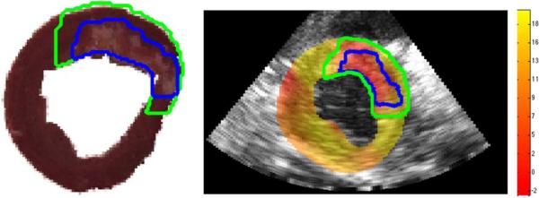
The sparse input displacements from shape tracking and speckle tracking are shown in Fig. 2(a). Fig. 2(b) shows the 3D radial strain map overlaid on the B-mode image with the infarct region identified. A sample accumulated displacement field is shown in Fig. 5. The displacement field accumulated to ES is overlaid on the ED B-mode image. Radial, circumferential, and longitudinal strain curves for a single canine for four short-axis slices in six regions are shown in Fig. 4. Abnormal strain curves were used to identify regions affected by the MI. For the canine in Fig. 4, the infarct was located primarily in the anterior segments. Some normal variability in peak strain values in each of the normal segments is expected [70].
Fig. 2.

(a) Sparse input vectors with shape tracking (red: epicardial, purple: endocardial), and speckle tracking (green). (b) Corresponding dense 3D myocardial radial strain map showing normal thickening in most regions (red for positive strain) and dyskinesis in the infarct (blue for negative strain) near ES.
Fig. 5.

Representative ED image for three perpendicular image planes of the ED B-mode image with segmentation (red) and accumulated displacements at ES overlaid (green).
Fig. 4.

Radial (solid), circumferential (dashed), and longitudinal (dotted) strain curves in percent strain derived from 4DE as a function of percent systole from a single representative canine six weeks post-MI.
Fig. 6 shows both radial and circumferential strain curves from four slices from MR tagging with corresponding slices from the full volume ultrasound strain data. The slices range from the apex to the base and the six segments correspond to those depicted in Fig. 3. We see that there is good correlation in the strain curves between the two methods for both radial and circumferential strains. The MRI strain results are subject to potential variability due to the difficulty of manually segmenting the tagged images.
Fig. 6.

Radial (positive) and circumferential (negative) strain curves in % derived from 4DE using our method (solid blue) and from MR tagging using HARP analysis (solid red) for a single post-occlusion dog at the four slices shown in Fig. 3 ranging from the apex to the base (top to bottom) divided into six segments from anteroseptal (left) to anterior (right) as a function of percent systole. Correlation coefficients between the two methods for both radial and circumferential strains are shown in the title of each frame. Infarct region is in the top right plots. Strains derived using an FFD approach (dashed blue) are shown for comparison.
Fig. 6 also shows multiple anterior LV wall segments with decreased radial strains. This pattern is consistent with the expected regional LV dysfunction after a MI due to LAD occlusion-reperfusion. Infarcted myocardial tissue in those segments results in the decreased contractility that is seen here.
Obtaining dense longitudinal strain information from MR requires either 3D tagging approaches or strain-encoded (SENC) imaging, which were not employed in the current study. These approaches are time-consuming and require specialized sequences that were not available. Using 2D conventional tagging and HARP (both of which are well-established methods), a sparse set of 4–6 long-axis slices is typically acquired. This, in turn, is not equivalent to the dense longitudinal strain information obtained by our integrated speckle and shape tracking approach. Nevertheless, the longitudinal strain values we obtained (reported here without comparison to MR) did show decreases consistent with post-MI LV dysfunction. Including all animals, mean end-systolic LS was –6.64% in the anterior mid-LV segment compared to –14.12% in a remote noninfarcted mid-LV segment.
Table I shows the median correlation coefficients for radial and circumferential strains from the combined approach outlined in Section II-D compared to the MR tagging strains for the six segments corresponding to the diagram in Fig. 7 for four short-axis slices shown in Fig. 3. Each correlation coefficient was computed by comparing MR tagging and 4DE-derived mean strain values at time points between ED and ES in the same anatomical segment for all dogs. Ultrasound provides much greater temporal resolution than MR and therefore the echo-derived strain curves were down-sampled to the temporal resolution of the MR. Short-axis slices and the segments within each slice were registered using anatomic landmarks seen in images from both modalities. We see strong correlation between the two methodologies with 75% of the correlation values being greater than 0.8 across the six segments at four slices in all dogs. The correlation coefficients are noted to be lowest in the apical anterior LV segments. This region always included infarcted tissue that led to decreased contractility and low strain magnitudes (often close to zero) that were more susceptible to noise with both imaging modalities.
TABLE I.
Median Correlation Coefficients for N = 8 Post-Occlusion Open-Chest Dogs Between Combined Method and MR Tagging for Six Sectors From Four Short Axis Slices Between the Apex and Base
| Anteroseptal | Inferoseptal | Inferior | Inferolateral | Anterolateral | Anterior | |||||||
|---|---|---|---|---|---|---|---|---|---|---|---|---|
| Combined | Radial | Circ. | Radial | Circ. | Radial | Circ. | Radial | Circ. | Radial | Circ. | Radial | Circ. |
| Apical | 0.86 | 0.87 | 0.87 | 0.97 | 0.95 | 0.81 | 0.84 | 0.95 | 0.77 | 0.90 | 0.70 | 0.66 |
| 0.92 | 0.93 | 0.93 | 0.97 | 0.88 | 0.79 | 0.85 | 0.86 | 0.67 | 0.89 | 0.81 | 0.95 | |
| 0.94 | 0.98 | 0.96 | 0.97 | 0.96 | 0.96 | 0.96 | 0.93 | 0.85 | 0.96 | 0.88 | 0.95 | |
| Basal | 0.96 | 0.96 | 0.96 | 0.97 | 0.96 | 0.98 | 0.92 | 0.96 | 0.90 | 0.98 | 0.91 | 0.97 |
In addition to correlation we also computed root-mean-square errors (RMSE) between the peak systolic strain values over all sectors and found that the RMSE (between 4DE and MR-tag) was 8.59% for the radial strain and 5.24% for the circumferential strain. We found the region with the largest RMSE in the radial direction to be the anteroseptal region, with an RMSE of 10.03%. This is likely due to the fact that radial motion in this segment is perpendicular to the ultrasound beam causing a greater variance in the calculated strain. The best agreement was found in the anterior region, where the RMSE in the radial direction was 4.95%. This is what we would expect because this region is closest to the ultrasound probe and the motion is in the axial direction. The circumferential strains were consistent across all six regions, with a max RMSE of 5.10% and a min of 3.18%.
To determine if any bias is present in the strain between 4DE-derived and MR tag-derived measurements, Bland–Altman analyses were performed for ES strain values from all eight dogs for four slices with six segments each. The Bland–Altman plots for radial and circumferential strains from 4DE and MR tagging are shown in Fig. 9. For radial strain, a mean difference of 1.09 strain was observed, with echo-derived values being slightly higher than MR-derived values. For circumferential strain, a mean difference of 1.38% strain was observed, with echo-derived values having slightly decreased magnitudes (of negative strain) compared to MR-derived values.
Fig. 9.

Bland–Altman plots for radial (top) and circumferential (bottom) end-systolic strain % for all eight dogs across four image slices in six image segments for ultrasound compared to MR. Mean difference (solid blue line) and 95% confidence interval (dashed blue line) are shown on the graphs.
The limits of agreement in the Bland–Altman plots are somewhat large. This could be the result of out-of-plane motion effects on MR-derived strain values that were calculated from 2D images. In contrast, echo-derived strain values were obtained from volumetric acquisitions and would not be affected by out-of-plane motion. Additionally, any registration errors made in selecting the anatomic slice subsets of echo-derived strains for comparison could lead to discrepancies. While tagged MR is recognized as providing reasonable estimates of strain, it does have limitations (especially with radial strain [70]) and there is no “gold standard” noninvasive technique [71]. Consequently, MR-derived strains should not be considered as ground truth and, where discrepancies exist, it is difficult to know which method is more accurate. We are planning experiments using implanted sonomicrometers to provide additional information about this question.
B. Comparison to Individual Methods
To compare the combined approach to the individual shape tracking and speckle tracking methods, we performed an analysis similar to our previously published 2D comparison [45], [46]. The adaptive radial basis function procedure was performed on the displacements from shape tracking alone, speckle tracking alone, and the combined values. Fig. 8 shows the correlations for the radial strain between shape combined approach and the two individual approaches. We see that the correlation values are good overall for the combined approach, as well as many of the segments for the individual methods. This is due to the processing that is performed on the raw displacement values by the radial basis function procedure. While the values for the individual methods are good, we can see that there are some regions where one of the individual methods performs poorly compared to the combined method. This shows the power of the combined approach. Similar analysis was performed on circumferential strains and the values were high for both individual and combined approaches.
Fig. 8.

Correlation coefficients for radial strain calculated from the combined method and MR (red), shape tracking alone and MR (blue), and speckle tracking alone and MR (green). Images were divided into six segments at four slices, as shown in Fig. 3. Columns of the figure represent the six segments around the myocardium with four correlation values in each column. Colored shading highlights the range of correlation values from the combined method (red) compared to the two individual methods (blue).
C. Comparison to Alternative Combined Technique (FFD)
To show the power of our adaptive RBF approach, we compared the strain values from our approach to those generated using a fixed-grid FFD approach for regularization. FFD approaches have been used to regularize the displacement field used to model the deformation fields in image registration-based tracking approaches [31], [32], [34]. To facilitate comparison, we performed regularization using FFD on the displacement values found with shape and speckle tracking derived from the same myocardial region used in the RBF approach.
The specific implementation in this work uses cubic B-spline functions for interpolation [72]. To ensure that a fair comparison is made between our method and the FFD method, an equal number of control points must be used. The adaptive RBF approach does not use the same number of control points for each image, so the average number of control points used for each volume over the cardiac cycle was found. One 4DE canine dataset was analyzed for this comparison. It had an average of 1421 control points over the cardiac cycle. To achieve a comparable number of control points for FFD, a fixed grid of 12 × 11 × 11 was used to give 1452 control points. The input displacement values to the FFD approach were the shape tracked displacements and the speckle tracked displacements with correlation coefficients above 0.6. The individual frame-to-frame dense displacement field was generated using FFD and accumulated using the same methods implemented for RBF in order to calculate cardiac coordinate strains. The strain values were then compared to the corresponding MR tagging strain values. A disadvantage of the fixed-regular grid of FFD is that control points will be located within the blood pool of the LV where there are no myocardial displacement values present.
Fig. 6 shows the radial and circumferential strain curves from RBF, FFD, and MR. There is a clear bias shown in the FFD plots. We can see that the FFD method underestimates the strain in both the radial and circumferential directions in comparison to the MR. To further investigate the differences between the methods, we compared the mean absolute difference between end-systolic strain values. The RBF approach was much closer to the values generated by MR. For circumferential strain, the mean difference compared to MR was 10.29% strain for FFD and 3.23% strain for RBF. Both ultrasound methods yielded lower magnitude circumferential strains than MR, but the RBF approach shows better agreement than the FFD approach. Future work could involve comparison to a multi-resolution FFD approach, but we believe that these initial results show the advantage of using RBF over FFD. A multi-resolution method would still require control points spaced on a regular grid or control points to be placed within the blood-pool that are required by FFD.
D. Comparison to Postmortem Images
After registration of the ultrasound images to the postmortem images, we are able to identify the infarct on the strain map derived from the ultrasound data. From the postmortem defined infarct zone, we define the peri-infarct zone by extending the infarct zone out by 5 mm. This resulted in peri-infarct volumes similar to those reported in the literature [73], [74]. A sample image showing a single slice from the full 3D volume of ES radial strains superimposed on the ED frame is shown in Fig. 11. In the strain image, we can see the decreased strain values within the infarct zone. The radial strains in the peri-infarcted zone are also seen to be lower than those in the remote noninfarcted tissue. For the same eight animals analyzed in the previous section mean ES strain in the radial, circumferential and longitudinal directions were found in the remote, border, and infarct regions of the myocardium. The results are shown in Table II. We can see that radial strain is best able to distinguish these three functional regions. There are large standard deviations due to differences in the infarct sizes across the eight dogs. The differences between the remote and border strains and the border and infarct strains were found to be statistically significant (p < 0.001) for all three strain directions using a paired-sample t-test for each. These comparisons all survive multiple comparison (Bonferroni) correction.
Fig. 11.
Slice of the postmortem heart with the infarct border (blue) and peri-infarct border (green) defined (left). Corresponding slice of the 3D radial strain map in percent strain overlaid on the B-mode image at the terminal time point with the mapped infarct border (blue) and peri-infarct (green) border warped to the B-mode image (right).
TABLE II.
Mean End-Systolic Strain for the Radial,Circumferential, and Longitudinal Directions for Remote, Border, and Infarct Tissue Regions Defined From Post-Mortem Image Slices
| Remote | Border | Infarct | ||||
|---|---|---|---|---|---|---|
| % Strain | STD | % Strain | STD | % Strain | STD | |
| Radial | 18.3 | 6.7 | 10.8 | 7.3 | 5.9 | 6.7 |
| Circ. | −11.39 | 1.52 | −8.35 | 3.43 | −8.05 | 5.64 |
| Long. | −15.4 | 5.9 | −14.7 | 5.6 | −11.2 | 16.1 |
Accurate strain estimation can help determine the distribution and severity of myocardial injury. This would provide valuable information for both diagnostic and therapeutic decision-making. While assessment of infarct size is obviously important, evaluation of surrounding tissue in the border or peri-infarct zone may also be helpful for monitoring pathophysiologic changes or for directing the administration of treatments [75], [76]. The low spatial resolution of MR tagging makes functional evaluation of the peri-infarct zone difficult. Anatomic MR or CT scans to identify infarct and border zones would require contrast administration (and associated complication risks) with either modality as well as radiation exposure with CT. Echocardiographic strain analysis can avoid these limitations while potentially providing important functional and anatomic information.
Much of the research literature has focused on longitudinal strain. While this measurement may be well suited for identifying myocardial dysfunction from an apical approach by taking advantage of high axial resolution, this may not be universally true. From a 3D parasternal short-axis view, radial strains will be associated with high axial resolution in the central regions of the acquisition while longitudinal strains will be associated with decreased resolution in a lateral direction. More so, these central radial strains will be unaffected by the lateral dropout that occurs, even with apical images, due to myocardial fiber orientations parallel to the ultrasound beam [71]. In the short axis view the motion parallel to the ultrasound beam in the center of the field of view is in the radial direction meaning that radial strain measurements could be very sensitive for detecting myocardial dysfunction. The relative scarcity of evidence supporting this may be due to current challenges in accurately assessing radial strains (especially in a lateral direction), rather than inherent physiologic factors. Our work aims to provide a more robust hybrid approach for strain determination that may be particularly useful in this setting.
V. Conclusion
In this work, we have presented an adaptive multi-level CSRBF approach for combining displacement information from shape and speckle tracking. We apply our methods to displacement values generated from shape tracking on myocardial boundaries and RF speckle tracking across the myocardium. We have shown that this combined approach correlates well to strain values derived from MR tagging. The combined approach performs better than either individual method when compared to MR tagging. Through a comparison with fixed grid FFD, we have shown that our adaptive approach is better than a single level approach on a fixed grid. The ability to noninvasively identify and quantify regional myocardial dysfunction is important for diagnosis and treatment planning. Through postmortem defined infarct, border, and remote regions we have shown that we are able to accurately identify regions of decreased contractility that correspond to prior myocardial infarctions. We have also shown that radial strain analysis can be useful in distinguishing infarct, border, and remote myocardial tissue regions.
Acknowledgment
The authors would like to thank C. Jia and L. Huang for their help with RF speckle tracking as well as Z. Zhang, K. Purushothaman, X. Hu, C. Hawley, X. Wang, M. Maxfield, and Z. Zhuang for assistance with data acquisition.
This work was supported in part by the National Institutes of Health (R01 HL082640, 5T32HL098069-03). The work of B. A. Lin was supported by an ASE Foundation Career Development Award.
Contributor Information
Colin B. Compas, IBM Research-Almaden, San Jose, CA 95120 USA..
Emily Y. Wong, Department of Bioengineering, University of Washington, Seattle, WA 98015 USA.
Xiaojie Huang, Department of Electrical Engineering, Yale University, New Haven, CT 06520 USA..
Smita Sampath, Department of Diagnostic Radiology, Yale University, New Haven, CT 06520 USA..
Ben A. Lin, Department of Internal Medicine, Yale University, New Haven, CT 06520 USA.
Prasanta Pal, Department of Diagnostic Radiology, Yale University, New Haven, CT 06520 USA..
Xenophon Papademetris, Departments of Diagnostic Radiology and Biomedical Engineering, Yale University, New Haven, CT 06520 USA..
Karl Thiele, Philips Medical Systems, Andover, MA 01810 USA..
Donald P. Dione, Department of Internal Medicine, Yale University, New Haven, CT 06520 USA.
Mitchel Stacy, Department of Internal Medicine, Yale University, New Haven, CT 06520 USA..
Lawrence H. Staib, Departments of Diagnostic Radiology, Electrical Engineering, and Biomedical Engineering, Yale University, New Haven, CT 06520 USA.
Albert J. Sinusas, Departments of Internal Medicine and Diagnostic Radiology, Yale University, New Haven, CT 06520 USA.
Matthew O'Donnell, Department of Bioengineering, University of Washington, Seattle, WA 98015 USA..
James S. Duncan, Departments of Diagnostic Radiology, Electrical Engineering, and Biomedical Engineering, Yale University, New Haven, CT 06520 USA.
References
- 1.Murray CJ, Jamison DT, Lopez AD, Ezzati M, Mathers CD. Global Burden of Disease and Risk Factors. World Bank, Oxford Univ. Press; Washington, DC: 2006. [PubMed] [Google Scholar]
- 2.Kramer C, Rogers W, Theobald T, Power T, Petruolo S, Reichek N. Remote noninfarcted region dysfunction soon after first anterior myocardial infarction. Circulation. 1996;94:660–666. doi: 10.1161/01.cir.94.4.660. [DOI] [PubMed] [Google Scholar]
- 3.Marcus JT, Götte MJ, Van Rossum AC, Kuijer JP, Heethaar RM, Axel L, Visser CA. Myocardial function in infarcted and remote regions early after infarction in man: Assessment by magnetic resonance tagging and strain analysis. Magn. Reson. Med. 1997 Nov.38:803–810. doi: 10.1002/mrm.1910380517. [DOI] [PubMed] [Google Scholar]
- 4.Kramer CM, Lima JA, Reichek N, Ferrari V. a., Llaneras MR, Palmon LC, Yeh IT, Tallant B, Axel L. Regional differences in function within noninfarcted myocardium during left ventricular remodeling. Circulation. 1993 Sep.88:1279–1288. doi: 10.1161/01.cir.88.3.1279. [DOI] [PubMed] [Google Scholar]
- 5.Bohs LN, Trahey GE. A novel method for angle independent ultrasonic imaging of blood flow and tissue motion. IEEE Biomed. Eng. 1991 Mar.38(3):280–286. doi: 10.1109/10.133210. [DOI] [PubMed] [Google Scholar]
- 6.Amundsen BH, Helle-Valle T, Edvardsen T, Torp H, Crosby J, Lyseggen E, Stoylen A, Ihlen H, Lima JC, Smiseth OA, Slordahl SA. Noninvasive myocardial strain measurement by speckle tracking echocardiography: Validation against sonomicrometry and tagged magnetic resonance imaging. J. Am. Coll. Cardiol. 2006 Feb.47:789–793. doi: 10.1016/j.jacc.2005.10.040. [DOI] [PubMed] [Google Scholar]
- 7.O'Donnell M, Skovoroda AR, Shapo BM, Emelianov SY. Internal displacement and strain imaging using ultrasonic speckle tracking. IEEE Trans. Ultrason., Ferroelectr. Freq. Control. 1994 May;41(3):314–325. [Google Scholar]
- 8.Lubinski M, Emelianov S, O'Donnell M. Speckle tracking methods for ultrasonic elasticity imaging using short-time correlation. IEEE Trans. Ultrason., Ferroelectr., Freq. Control. 1999 Jan.46(1):82–96. doi: 10.1109/58.741427. [DOI] [PubMed] [Google Scholar]
- 9.Ma C, Varghese T. Comparison of cardiac displacement and strain imaging using ultrasound radiofrequency and envelope signals. Ultrasonics. 2013 Mar.53:782–792. doi: 10.1016/j.ultras.2012.11.005. [DOI] [PMC free article] [PubMed] [Google Scholar]
- 10.Lopata RG, Nillesen MM, Thijssen JM, Kapusta L, de Korte CL. Three-dimensional cardiac strain imaging in healthy children using RF-data. Ultrasound Med. Biol. 2011 Sep.37:1399–1408. doi: 10.1016/j.ultrasmedbio.2011.05.845. [DOI] [PubMed] [Google Scholar]
- 11.Kaluzynski K, Chen X, Emelianov SY, Skovoroda AR, O'Donnell M. Strain rate imaging using two-dimensional speckle tracking. IEEE Trans. Ultrason., Ferroelectr. Freq. Control. 2001 Jul.48(4):1111–1123. doi: 10.1109/58.935730. [DOI] [PubMed] [Google Scholar]
- 12.Lee W-N, Qian Z, Tosti CL, Brown TR, Metaxas DN, Konofagou EE. Preliminary validation of angle-independent myocardial elastography using MR tagging in a clinical setting. Ultrasound Med. Biol. 2008 Dec.34:1980–1997. doi: 10.1016/j.ultrasmedbio.2008.05.007. [DOI] [PMC free article] [PubMed] [Google Scholar]
- 13.Lee W-N, Provost J, Fujikura K, Wang J, Konofagou EE. In vivo study of myocardial elastography under graded ischemia conditions. Phys. Med. Biol. 2011 Mar.56:1155–1172. doi: 10.1088/0031-9155/56/4/017. [DOI] [PMC free article] [PubMed] [Google Scholar]
- 14.Konofagou E, Lee W-N, Luo J, Provost J, Vappou J. Physiologic cardiovascular strain and intrinsic wave imaging. Annu. Rev. Biomed. Eng. 2011 Aug.13:477–505. doi: 10.1146/annurev-bioeng-071910-124721. [DOI] [PubMed] [Google Scholar]
- 15.Duan Q, Angelini E, Gerard O, Homma S, Laine A. Comparing optical-flow based methods for quantification of myocardial deformations on RT3D ultrasound. Proc. IEEE Int. Symp. Biomed. Imag.: Nano to Macro. 2006:173–176. [Google Scholar]
- 16.Horn B, Schunck B. Determing optical flow. Artif. Intell. 1981;17:185–203. [Google Scholar]
- 17.Lucas B, Kanade T. An iterative image registration technique with an application to stereo vision. Proc. DARPA Image Understand. Workshop. 1981:121–130. [Google Scholar]
- 18.Song SM, Leahy RM. Computation of 3-D velocity fields from 3-D cine CT images of a human heart. IEEE Trans. Med. Imag. 1991 Jan.10(1):295–306. doi: 10.1109/42.97579. [DOI] [PubMed] [Google Scholar]
- 19.Papademetris X, Sinusas A, Dione D. Estimation of 3D left ventricular deformation from echocardiography. Med. Image Anal. 2001 Mar.5:17–28. doi: 10.1016/s1361-8415(00)00022-0. [DOI] [PubMed] [Google Scholar]
- 20.Lin N, Duncan J. Generalized robust point matching using an extended free-form deformation model: Application to cardiac images. Proc. 2004 IEEE Int. Symp. Biomed. Imag.: From Nano to Macro. 2004:320–323. [Google Scholar]
- 21.Besl PJ, McKay ND. A method for registration of 3-D shapes. IEEE Trans. Pattern Anal. Mach. Intell. 1992 Feb.14(2):239–256. [Google Scholar]
- 22.Rusinkiewicz S, Levoy M. Efficient variants of the ICP algorithm. 3-D Digital Imag. Model. 2001 [Google Scholar]
- 23.Rangarajan A, Chui H, Mjolsness E, Pappu S, Davachi L, Goldman-Rakic P, Duncan J. A robust point-matching algorithm for autoradiograph alignment. Med. Image Anal. 1997 Sep.1:379–398. doi: 10.1016/s1361-8415(97)85008-6. [DOI] [PubMed] [Google Scholar]
- 24.Myronenko A, Song X, Carreira-Perpinan M. Non-rigid point set registration: Coherent point drift. IEEE Trans. Pattern Anal. Mach. Intell. 2010 Dec.32:2262–2275. doi: 10.1109/TPAMI.2010.46. [DOI] [PubMed] [Google Scholar]
- 25.Zerhouni E, Parish D, Rogers W, Yang A. Human heart: Tagging with MR imaging—A method for noninvasive assessment of myocardial motion. Radiology. 1988;(2):59–63. doi: 10.1148/radiology.169.1.3420283. [DOI] [PubMed] [Google Scholar]
- 26.Axel L, Dougherty L. MR imaging of motion with spatial modulation of magnetization. Radiology. 1989:841–845. doi: 10.1148/radiology.171.3.2717762. [DOI] [PubMed] [Google Scholar]
- 27.Osman NF, Prince JL. Visualizing myocardial function using HARP MRI. Phys. Med. Biol. 2000 Jun;45:1665–1682. doi: 10.1088/0031-9155/45/6/318. [DOI] [PubMed] [Google Scholar]
- 28.Epstein FH. MRI of left ventricular function. J. Nucl. Cardiol. 2007;14(5):729–744. doi: 10.1016/j.nuclcard.2007.07.006. [DOI] [PubMed] [Google Scholar]
- 29.Ryf S, Spiegel MA, Gerber M, Boesiger P. Myocardial tagging with 3D-CSPAMM. J. Magn. Reson. Imag. 2002 Sep.16:320–325. doi: 10.1002/jmri.10145. [DOI] [PubMed] [Google Scholar]
- 30.Sederberg TW, Parry SR. Free-form deformation of solid geometric models. ACM SIGGRAPH Comput. Graph. 1986;20(4) [Google Scholar]
- 31.Ledesma-Carbayo MJ, Kybic J, Desco M, Santos A, Sühling M, Hunziker P, Unser M. Spatio-temporal nonrigid registration for ultrasound cardiac motion estimation. IEEE Trans. Med. Imag. 2005 Sep.24(9):1113–1126. doi: 10.1109/TMI.2005.852050. [DOI] [PubMed] [Google Scholar]
- 32.Elen A, Choi HF, Loeckx D, Gao H, Claus P, Suetens P, Maes F, D'hooge J. Three-dimensional cardiac strain estimation using spatio-temporal elastic registration of ultrasound images: A feasibility study. IEEE Trans. Med. Imag. 2008 Nov.27(11):1580–1591. doi: 10.1109/TMI.2008.2004420. [DOI] [PubMed] [Google Scholar]
- 33.De Craene M, Piella G, Camara O, Duchateau N, Silva E, Doltra A, D'hooge J, Brugada J, Sitges M, Frangi AF. Temporal diffeomorphic free-form deformation: Application to motion and strain estimation from 3D echocardiography. Med. Image Anal. 2012 Feb.16:427–450. doi: 10.1016/j.media.2011.10.006. [DOI] [PubMed] [Google Scholar]
- 34.Heyde B, Cygan S, Choi HF, Lesniak-Plewinska B, Barbosa D, Elen A, Claus P, Loeckx D, Kaluzynski K, D'hooge J. Regional cardiac motion and strain estimation in three-dimensional echocardiography: A validation study in thick-walled univentricular phantoms. IEEE Trans. Ultrason., Ferroelectr. Freq. Control. 2012 Apr.59(4):668–882. doi: 10.1109/TUFFC.2012.2245. [DOI] [PubMed] [Google Scholar]
- 35.Myronenko A, Song X, Sahn D. Maximum likelihood motion estimation in 3D echocardiography through non-rigid registration in spherical coordinates. Funct. Imag. Model. Heart. 2009:427–436. [Google Scholar]
- 36.Coquillart S. Extended free-form deformation: A sculpturing tool for 3D geometric modeling. ACM SIGGRAPH Comput. Graph. 1990 Sep.24:187–196. [Google Scholar]
- 37.Shi P, Sinusas A, Constable R, Duncan J. Volumetric deformation analysis using mechanics-based data fusion: Applications in cardiac motion recovery. Int. J. Comput. Vis. 1999;35(1):87–107. [Google Scholar]
- 38.Clough R, Tocher J. Finite element stiffness matrices for analysis of plates in bending. Proc. Conf. Matrix Methods Struct. Mechan. 1965:515–545. [Google Scholar]
- 39.Brebbia CA, Wrobel LC. The boundary element method. Comput. Methods Fluids. 1980:26–48. [Google Scholar]
- 40.Yan P, Lin N, Sinusas AJ, Duncan JS. A boundary element-based approach to analysis of LV deformation. Med. Image Comput. Comput. Assist. Intervent. 2005 Jan.8:778–785. doi: 10.1007/11566465_96. [DOI] [PubMed] [Google Scholar]
- 41.Rohde GK, Aldroubi A, Dawant BM. The adaptive bases algorithm for intensity-based nonrigid image registration. IEEE Trans. Med. Imag. 2003 Nov.22(11):1470–1479. doi: 10.1109/TMI.2003.819299. [DOI] [PubMed] [Google Scholar]
- 42.Bistoquet A, Oshinski J, Skrinjar O. Myocardial deformation recovery from cine MRI using a nearly incompressible biventricular model. Med. Image Anal. 2008 Feb.12:69–85. doi: 10.1016/j.media.2007.10.009. [DOI] [PubMed] [Google Scholar]
- 43.Huang SW, Rubin JM, Xie H, Witte RS, Jia C, Olafsson R, O'Donnell M. Analysis of correlation coefficient filtering in elasticity imaging. IEEE Trans. Ultrason., Ferroelectr. Freq. Control. 2008 Nov.55(11):2426–2441. doi: 10.1109/TUFFC.950. [DOI] [PubMed] [Google Scholar]
- 44.Lubinski M, Emelianov SY, Raghavan K, Yagle A, Skovoroda A, O'Donnell M. Lateral displacement estimation using tissue incompressibility. IEEE Trans. Ultrason., Ferroelectr. Freq. Control. 1996 Mar.43(2):247–256. doi: 10.1109/58.660158. [DOI] [PubMed] [Google Scholar]
- 45.Compas CB, Lin BA, Sampath S. Combining shape and speckle tracking for deformation analysis in echocardiography using radial basis functions. Proc. IEEE Int. Symp. Biomed. Imag.: From Nano to Macro. 2011:1322–1325. [Google Scholar]
- 46.Compas CB, Lin BA, Sampath S, Jia C, Wei Q, Sinusas AJ, Duncan JS. Functional Imaging and Modeling of the Heart. Springer; New York: 2011. Multi-frame radial basis functions to combine shape and speckle tracking for cardiac deformation analysis in echocardiogramation analysis in echocardiographyphy; pp. 113–120. [Google Scholar]
- 47.Compas CB, Lin BA, Sampath S, Huang L, Wei Q, Sinusas AJ, Duncan JS. Comparing shape tracking, speckle tracking, a combined method for deformation analysis in echocardiography. Proc. 1st IEEE Int. Conf. Healthcare Informat., Imag. Syst. Biol. 2011 Jul.:120–125. [Google Scholar]
- 48.Compas CB, Wong EY, Huang X, Sampath S, Lin BA, Papademetris X, Thiele K, Dione DP, Sinusas AJ, O'Donnell M, Duncan JS. A combined shape tracking and speckle tracking approach for 4d deformation analysis in echocardiography. Proc. 2012 IEEE Int. Symp. Biomed. Imag.: From Nano to Macro. 2012 May;:458–461. [Google Scholar]
- 49.Pearlman PC, Tagare TD, Lin BA, Sinusas AJ, Duncan JS. Segmentation of 3d radio frequency echocardiography using a spatio-temporal predictor. Med. Image Anal. 2011;16(2):351–360. doi: 10.1016/j.media.2011.09.002. [DOI] [PMC free article] [PubMed] [Google Scholar]
- 50.Bosch JG, Mictchell SC, Lelieveldt BPF, Nijland F, Kamp O, Sonka M, Reiber JHC. Automatic segmentation of echocardio-graphic sequences by active appearance motion models. IEEE Trans. Med. Imag. 2002 Nov.21(11):1374–1382. doi: 10.1109/TMI.2002.806427. [DOI] [PubMed] [Google Scholar]
- 51.Sun W, Çetin M, Chan RC, Reddy VY, Holmvang G, Chandar V, Willsky AS. Segmenting and tracking the left ventricle by learning the dynamics in cardiac images. In: Christensen GE, Sonka M, editors. Information Processing in Medical Imaging. Vol. 3565. Springer; New York: 2005. pp. 553–565. LNCS. [DOI] [PubMed] [Google Scholar]
- 52.Zhu Y, Papademetris X, Sinusas AJ, Duncan JS. A dynamical shape prior for LV segmentation from RT3D echocardiography. In: Yang G-Z, Hawkes DJ, Rueckert D, Noble JA, Taylor CJ, editors. Medical Image Computing and Computer Assisted Intervention. Vol. 5761. Springer; New York: 2009. pp. 206–213. LNCS. [DOI] [PMC free article] [PubMed] [Google Scholar]
- 53.Yang L, Georgescu B, Zheng Y, Meer P, Comaniciu D. 3d ultrasound tracking of the left ventricle using one-step forward prediction and data fusion of collaborative trackers. Proc. IEEE Conf. Comput. Vis. Pattern Recognit. 2008 Jun.:1–8. [Google Scholar]
- 54.Huang X, Lin BA, Compas CB, Sinusas AJ, Staib LH, Duncan JS. Segmentation of left ventricles from echocardiographic sequences via sparse appearance representation. Proc. IEEE Workshop Math. Methods Biomed. Image Anal. 2012 Jan.:305–312. [Google Scholar]
- 55.Huang X, Dione DP, Compas CB, Papademetris X, Lin BA, Sinusas AJ, Duncan JS. A dynamical appearance model based on multiscale sparse representation: Segmentation of the left ventricle from 4d echocardiography. Med. Image Comput. Comput. Assist. Intervent. 2012:58–65. doi: 10.1007/978-3-642-33454-2_8. [DOI] [PMC free article] [PubMed] [Google Scholar]
- 56.Freund Y, Schapire R. A Desicion-Theoretic Generalization of on-Line Learning and an Application to Boosting. Vol. 904. Springer; New York: 1995. pp. 23–37. LNCS. [Google Scholar]
- 57.Aharon M, Elad M, Bruckstein A. K-SVD: An algorithm for designing overcomplete dictionaries for sparse representation. IEEE Trans. Signal Process. 2006 Nov.54(11):4311–4322. [Google Scholar]
- 58.Papademetris X, Sinusas AJ, Dione DP, Constable RT, Duncan JS. Estimation of 3-D left ventricular deformation from medical images using biomechanical models. IEEE Trans. Med. Imag. 2002 Jul.21(7):786–800. doi: 10.1109/TMI.2002.801163. [DOI] [PubMed] [Google Scholar]
- 59.Shi P, Sinusas AJ, Constable RT, Ritman E, Duncan JS. Point-tracked quantitative analysis of left ventricular surface motion from 3-D image sequences. IEEE Trans. Med. Imag. 2000 Jan.19(1):36–50. doi: 10.1109/42.832958. [DOI] [PubMed] [Google Scholar]
- 60.Jia C, Yan P, Sinusas A, Dione DP, Lin B, Wei Q, Thiele K, Theodore J, Rubin J, Huang L, Duncan J, O'Donnell M. 3D elasticity imaging using principal stretches on an open-chest dog heart. Proc. 2010 IEEE Ultrason. Symp. 2010:583–586. [Google Scholar]
- 61.Loupas T, Powers J, Gill R. An axial velocity estimator for ultrasound blood flow imaging, based on a full evaluation of the Doppler equation by means of a two-dimensional autocorrelation approach. IEEE Trans. Ultrason., Ferroelectr. Freq. Control. 1995 Jul.42(4):672–688. [Google Scholar]
- 62.Wendland H. Piecewise polynomial, positive definite and compactly supported radial functions of minimal degree. Adv. Comput. Math. 1995 Dec.4:389–396. [Google Scholar]
- 63.Buhmann M. Radial Basis Functions: Theory and Implementations. Cambridge Univ. Press; Cambridge, U.K.: 2003. [Google Scholar]
- 64.Reimer KA, Lowe JE, Rasmussen MM, Jennings RB. The wavefront phenomenon of ischemic cell death. 1. Myocardial infarct size vs duration of coronary occlusion in dogs. Circulation. 1977 Nov.56:786–794. doi: 10.1161/01.cir.56.5.786. [DOI] [PubMed] [Google Scholar]
- 65.Yan P, Sinusas A, Duncan JS. Boundary element method-based regularization for recovering of LV deformation. Med. Image Anal. 2007 Dec.11:540–554. doi: 10.1016/j.media.2007.04.007. [DOI] [PubMed] [Google Scholar]
- 66.Young AA, Imai H, Chang CN, Axel L. Two-dimensional left ventricular deformation during systole using magnetic resonance imaging with spatial modulation of magnetization. Circulation. 1994 Feb.89:740–752. doi: 10.1161/01.cir.89.2.740. [DOI] [PubMed] [Google Scholar]
- 67.Osman NF, Kerwin WS, McVeigh ER, Prince JL. Cardiac motion tracking using CINE Harmonic Phase (HARP) magnetic resonance imaging. Magn. Reson. Med. 1999;42(6):1048–1060. doi: 10.1002/(sici)1522-2594(199912)42:6<1048::aid-mrm9>3.0.co;2-m. [DOI] [PMC free article] [PubMed] [Google Scholar]
- 68.Duncan J, Papademetris X, Yang J, Jackowski M, Zeng X, Staib LH. Geometric strategies for neuroanatomical analysis from MRI. NeuroImage. 2004;23:S34–S45. doi: 10.1016/j.neuroimage.2004.07.027. [DOI] [PMC free article] [PubMed] [Google Scholar]
- 69.Papademetris X, Jackowski M, Rajeevan N, Constable R, Staib L. BioImage Suite: An integrated medical image analysis suite Sect. Bioimag. Sci., Dept. Diagnostic Radiol., Yale School Med. [Online] Available: http://www.bioimagesuite.org.
- 70.Moore CC, Lugo-Olivieri CH, McVeigh ER, Zerhouni EA. Three-dimensional systolic strain patterns in the normal human left ventricle: Characterization with tagged MR imaging. Radiology. 2000;214(2):453–466. doi: 10.1148/radiology.214.2.r00fe17453. [DOI] [PMC free article] [PubMed] [Google Scholar]
- 71.Mor-Avi V, Lang RM, Badano LP, Belohlavek M, Cardim NM, Derumeaux G, Galderisi M, Marwick T, Nagueh SF, Sengupta PP, et al. Current and evolving echocardiographic techniques for the quantitative evaluation of cardiac mechanics: ASE/EAE consensus statement on methodology and indications: Endorsed by the Japanese society of echocardiography. J. Am. Soc. Echocardiogr. 2011;24(3):277–313. doi: 10.1016/j.echo.2011.01.015. [DOI] [PubMed] [Google Scholar]
- 72.Bardinet E, Cohen LD, Ayache N. A parametric deformable model to fit unstructured 3D data. Comput. Vis. Image Understand. 1998 Jul.71:39–54. [Google Scholar]
- 73.Peters DC, Appelbaum EA, Nezafat R, Dokhan B, Han Y, Kissinger KV, Goddu B, Manning WJ. Left ventricular infarct size, peri-infarct zone, papillary scar measurements: A comparison of high-resolution 3D and conventional 2D late gadolinium enhancement cardiac MR. J. Magn. Reson. Imag. 2009 Oct.30:794–800. doi: 10.1002/jmri.21897. [DOI] [PMC free article] [PubMed] [Google Scholar]
- 74.Yan AT, Shayne AJ, Brown KA, Gupta SN, Chan CW, Luu TM, Di Carli MF, Reynolds HG, Stevenson WG, Kwong RY. Characterization of the peri-infarct zone by contrast-enhanced cardiac magnetic resonance imaging is a powerful predictor of post-myocardial infarction mortality. Circulation. 2006 Jul.114:32–39. doi: 10.1161/CIRCULATIONAHA.106.613414. [DOI] [PubMed] [Google Scholar]
- 75.McCain ML, Parker KK. Mechanotransduction: The role of mechanical stress, myocyte shape, cytoskeletal architecture on cardiac function. Eur. J. Physiol. 2011 Jul.462:89–104. doi: 10.1007/s00424-011-0951-4. [DOI] [PubMed] [Google Scholar]
- 76.Schuleri KH, Centola M, Evers KS, Zviman A, Evers R, Lima J. a. A., Lardo AC. Cardiovascular magnetic resonance characterization of peri-infarct zone remodeling following myocardial infarction. J. Cardiovasc. Magn. Reson. 2012 Jan.14:24. doi: 10.1186/1532-429X-14-24. [DOI] [PMC free article] [PubMed] [Google Scholar]