Spatial patterns of genome‐wide expression profiles reflect anatomic and fiber connectivity architecture of healthy human brain

Abstract

Unraveling the relationship between molecular signatures in the brain and their functional, architectonic, and anatomic correlates is an important neuroscientific goal. It is still not well understood whether the diversity demonstrated by histological studies in the human brain is reflected in the spatial patterning of whole brain transcriptional profiles. Using genome‐wide maps of transcriptional distribution of the human brain by the Allen Brain Institute, we test the hypothesis that gene expression profiles are specific to anatomically described brain regions. In this work, we demonstrate that this is indeed the case by showing that gene similarity clusters appear to respect conventional basal‐cortical and caudal‐rostral gradients. To fully investigate the causes of this observed spatial clustering, we test a connectionist hypothesis that states that the spatial patterning of gene expression in the brain is simply reflective of the fiber tract connectivity between brain regions. We find that although gene expression and structural connectivity are not determined by each other, they do influence each other with a high statistical significance. This implies that spatial diversity of gene expressions is a result of mainly location‐specific features but is influenced by neuronal connectivity, such that like cellular species preferentially connects with like cells. Hum Brain Mapp 35:4204–4218, 2014. © 2014 Wiley Periodicals, Inc.

INTRODUCTION

A major goal of neurological research is to understand the nature and causes of molecular, functional [Johnson et al., 2009] and architectonic [Swanson, 2000] diversity in the brain. Gene expression profiling [Schena et al., 1995; Shalon et al., 1996] is a powerful means to explore the molecular‐cellular basis of the spatial diversity of brain cells [Lein et al., 2007] as their differential phenotypic properties result from unique combinations of genotypes. Mouse brain atlases of gene expression showing inter‐regional differences of structure and function point to their molecular basis [Bohland et al., 2010; French and Pavlidis, 2011; French et al., 2011; Grange and Mitra, n.d.; Sunkin and Hohmann, 2007; Wolf et al., 2011; Zapala et al., 2005]. The spatial patterns of gene expression in mouse appear to match anatomic organization but few studies have explored these relationships in human data due to challenges in acquisition, limited number of samples and the destructive nature of molecular assays [Hawrylycz et al., 2012].

In this article, we interrogate the relationship between spatial patterning of gene expression and anatomic/functional boundaries in the human brain. We pose and rigorously test two specific hypotheses. First, we ask whether gene expression in the human brain is spatially clustered in a manner reflective of brain anatomy. Our main contribution is the application of a novel non‐linear dimensionality reduction algorithm based on manifold learning to discover spatial correlations in the genetic signature of different locations in the human brain, using the Allen Human Brain Atlas (ABA) [Jones et al., 2009] produced by the Allen Brain Institute (ABI), which provides microarray expression profiles of almost every gene of the human genome at hundreds of locations in the brain. We find strong evidence for the hypothesis that gene expression clusters are spatially segregated and reveal large‐scale organization of the human brain. Three distinct anatomic regions cluster together, roughly conforming to cytoarchitectonic groupings—a cerebellum/striatum/basal group, a posterior/occipital/medial cortical group, and a frontal cortical group. These findings are consistent with a recent study by ABI [Hawrylycz et al., 2012], which shows how transcriptional regulation varies enormously with anatomic location. These results represent the human analogue of caudal‐rostral clustering along the neural tube reported in animals [Bernard et al., 2012; Zapala et al., 2005].

Next, we explore whether regions that are structurally connected by white matter tracts have similar gene expression levels. Expression signature of C. elegans [Kaufman et al., 2006] and mouse neurons [French and Pavlidis, 2011; French et al., 2011] appear to carry significant information about its synaptic connectivity. Surprisingly, we found no evidence that structural connectivity, determined by MR diffusion tractography [Iturria‐Medina et al., 2005], determines gene similarity in the human brain. However, this method of exploring the expression‐connection question inappropriately assumes independence among brain regions. Instead, we set up a precise but more general hypothesis test by considering the entire network rather than individual connections independently. To our knowledge, this formulation has not been reported before. We find that although no inter‐regional connection is determined solely by gene similarity between them, the overall connectivity network conforms to inter‐regional gene similarity data in a way that cannot arise by chance. Thus, gene expression influences rather than strictly determines structural connectivity. Taken together, our results point to a molecular ontology of the human brain.

MATERIALS AND METHODS

Allen Brain Atlas Data

Genome‐wide ABA microarray expression data from two postmortem brains (H0351.2001 and H0351.2002) obtained at 946 and 896 distinct brain locations, respectively, provided complete anatomic coverage of the brain. The data was reformatted into two ( $\text{brainregion} \times \text{gene}\hspace{0.17em}$) matrices of size $946\times 58,000$ and $896\times 58,000$. Gene expression profiles from all locations within each of 323 distinct brain structures, identified using histopathological labels provided by ABI were averaged prior to performing spatial clustering.

Dimensionality Reduction

Given the extremely large number of genes involved, we implemented two dimensionality reduction schemes: conventional Singular Value Decomposition (SVD) and non‐linear Generalized Discriminant Analysis (GDA) [Singh and Silakari, 2009; Ye, 2005]. GDA is the reformulation of Linear Discriminant Analysis (LDA) [Fisher, 1936] in high‐dimensional space, constructed using a kernel function [Schaeffer, 2007]. Both methods transform high‐dimensional data into a meaningful representation of reduced dimensionality, a common procedure in gene expression data analysis to mitigate the curse of dimensionality and facilitate classification, visualization, and compression of under‐sampled but high‐dimensional microarray data. Nonlinear mappings like GDA are particularly useful when linear mappings are unable to reveal separability in data [Krzanowskit, 1995]. The first five dominant singular components were retained in the SVD analysis [Alter et al., 2000] of the $\text{brainregion} \times \text{gene}\hspace{0.17em}$ matrix (after removing the first component which simply captures mean expression). These five components, representing 98% of the variance, were used to reconstruct “reduced” matrices of size $946\times 5$ and $896\times 5$, respectively. Five components were chosen as this was the smallest number at which stable clusters were formed (see below for definition of stable), after testing 2–20 components. A similar procedure was applied using GDA [Singh and Silakari, 2009; Ye, 2005]; a Gaussian kernel was selected for subsequent analysis after experimentation with different kernels (linear, polynomial, and Gaussian).

All computations and visualizations were performed using Matlab (MATLAB 2011a). The above processes are common to both hypotheses 1 and 2, but the subsequent steps that vary are described below.

Specific Methods for Hypothesis 1

Obtaining gene similarity matrix

The next step was to convert the reduced $\text{brainregion} \times \text{gene}\hspace{0.17em}$ data into a $\text{brainregion} \times \text{gene}\hspace{0.17em}$ similarity matrix (or graph), whose ${(i,j)}^{\text{th}\hspace{0.17em}}$ element is given by the similarity in gene expression between regions $i$ and $j$. We did this so that we can apply graph clustering algorithms to the resulting similarity graph and obtain clusters of regions with similar gene expression. For this purpose, we chose the most commonly used similarity metric—Pearson's correlation coefficient.

Graph or spectral clustering

Spectral clustering uses information obtained from the eigenvalues and eigenvectors of adjacency matrices for graph partitioning [Schaeffer, 2007]. It approximates the sparsest cut of a graph through the second eigenvalue of its Laplacian [Smola and Kondor, 2003]. Spectral clustering methods find a cut through a connected graph such that the nodes within each cluster are tightly connected to each other and loosely connected to nodes in other clusters. They are especially powerful for high‐dimensional data, which may be clustered on a nonlinear manifold (as compared to a linear subspace in feature space, which would be easy to separate by linear techniques). It has been found that for gene expression data, multiway spectral clustering algorithms are the most stable of all clustering algorithms [Auffarth, 2007]. We used the algorithm by Jordan and Weiss [Ng and Jordan, 2002], which relies on the eigen‐decomposition of the Laplacian of the graph (defined as the difference of the degree matrix and the adjacency matrix), followed by a conventional k‐means clustering algorithm [Ng and Jordan, 2002].

Repeated seeding and majority vote

k‐means clustering requires an initial cluster assignment. Because the final clusters depend on the initial guess, a large number of trials with randomized initial guesses (called seeding) were typically performed. Unfortunately, randomized seeding of the k‐means spectral clustering algorithm ([Ng and Jordan, 2002] does not in general guarantee a unique clustering in repeated trials. If an outlier was chosen as an initial seed, then no other vector was assigned to it during subsequent iterations, giving a singleton cluster (a cluster with only one point). Poor initial seeding could also result in empty clusters. To overcome this problem, clustering was repeated 100 times and a majority vote was taken. This majority vote generally gave the most likely and stable clustering, i.e., the one that is repeatedly generated in most trials).

Finding exemplar genes

After spectral clustering and choosing the best results with three clusters, backtracking was performed to identify genes that might be responsible for spatial clustering. The $58,000\times 1$ gene vectors for each cluster were found and then ranked according to ascending P values after three paired t tests between the clusters. The top 10 genes from each paired test were then identified as genes that might be driving the spatial clustering.

Specific Methods for Hypothesis 2

The hypothesis testing the connection between gene expression and connectivity required whole brain structural connectivity data. We denote the extent of white matter fiber connectivity between two regions $i$ and $j$ by $c_{i,j}$, and let the matrix $C=\{c_{i,j}|i,j\in [1,N]\}$ represent the whole brain connectivity matrix. This information was obtained from diffusion MRI scans of the brain, followed by tractography and network extraction imposed upon a parcellated brain atlas using previously published methods [Ivković et al., 2012; Kuceyeski et al., 2011].

Formation of a new 219‐region brain atlas

To construct a parcellated atlas faithful both to the ABI's gene sample locations as well as to prior tractography‐based analyses, we constructed a new atlas as follows. We began with the 116‐region Automatic Anatomic Labeling (AAL) [Tzourio‐Mazoyer et al., 2002] brain atlas, available in standardized Montreal Neurological Institute (MNI) space, upon which we imposed further substructure parcellations to obtain a new atlas whose region sizes are roughly equal. To do this, we sliced each of the cortical regions in the original AAL atlas along the principal axis, taking care to not create a region that was smaller than a certain threshold, leaving subcortical regions untouched. This resulted in a 219‐region atlas; the genetic expression of points within the same region was averaged.

Diffusion tensor imaging, tractography, and brain network extraction

T1‐weighted structural MR and high angular resolution diffusion imaging (HARDI) data were collected on 14 healthy adults on a 3 Tesla GE Signa EXCITE scanner (GE Healthcare, Waukesha, WI). HARDI data were acquired from 55 isotropically distributed diffusion‐encoding directions at b = 1,000 s mm⁻² and one at b = 0 s mm⁻², with 72 1.8‐mm‐thick slices and $0.9\times 0.9$ mm² in‐plane resolution. The structural scan was an axial 3D inversion recovery fast spoiled gradient recalled echo (FSPGR) T1 weighted images (TE = 1.5 ms, TR = 6.3 ms, TI = 400 ms, flip angle of 15°) with $0.9\times 0.9\times 1$ mm³ resolution. The above 219‐region atlas was co‐registered onto each subject's structural MR volume using the individual brain atlases using statistical parametric mapping (IBASPM) [Aleman‐Gomez et al., 2006] and statistical parametric mapping (SPM5) [Friston et al., 2006] software packages in MATLAB. The resulting image was then co‐registered to the subject's diffusion space and the voxels at the gray/white interface were seeded for MR diffusion probabilistic tractography by drawing 50 seeds in each interface voxel [Iturria‐Medina et al., 2005]. Structural connectivity between any two gray matter structures in the 219‐region atlas was taken to be its Anatomical Connection Strength (ACS), which is a sum of tractography‐derived streamlines connecting two regions, weighted by each streamline's probability. The ACS is a proxy for the cross‐sectional area of connecting nerve fibers and was claimed to represent potential information flow between regions [Iturria‐Medina et al., 2008]. The mean ACS value over all 14 subjects was used to populate the connectivity matrix C, after removing possibly spurious connections identified by a conventional hypothesis test applied separately to each connection. Entries for which the z‐scores were below the (P < 0.001) threshold across the healthy normal ACS connectivity values were removed. This method of removing spurious connections was introduced in [Ivković et al., 2012], who also applied a statistical threshold of P = 0.001.

Formulating a testable brain connectivity—Gene expression hypothesis

This hypothesis was formulated as a precise mathematical problem in the following way. First, we let $g_i$ represent a vector containing the gene expression values for region $i$. Gene filtering was used to obtain a reduced “spatial‐eigengene” vector $x_i$. We denoted the collection of eigen‐genes from all brain regions by $x=\{x_i|i\in [1,N]\}$. We hypothesized that the gene expression in region $i$ was given simply by a linear combination of gene expressions in all regions structurally connected to it, and the influence of region $j$ to region $i$'s expression was proportional to the connectivity (ACS) between them, i.e. $c_i,j$. Thus

$$x_i={\displaystyle \sum _{j|(i,j)\in {\rm A}}{c}_i,ixj+{\zeta }_i,}$$

where the random signal ${\zeta }_i$ allowed each region to have a unique gene signature not shared by any other region. For the gene‐connectivity relation to hold, this unique signal must be independent and identically distributed (i.i.d.), i.e., an “innovation” signal. In addition, it should have a small norm compared to the overall gene expression data so that majority of the expression signal is accounted for by connectivity relationships. Expanding the above equation to all brain regions, we got

$$x=Cx+\zeta$$

where we collected all region‐wise innovation signals into $\zeta$. This gave

$$\zeta =(I-C)x=Lx$$

where $L=I-C$ is the normalized Laplacian of the connectivity matrix $C$.

This gene‐connectivity model implies that, given the connectivity matrix and the gene expression data, the matrix‐vector product $Lx$ must be i.i.d. with its covariance matrix given by the identity matrix.

Statistical Test to Determine Validity of the Hypothesis

We wish to test the condition that $E(\zeta {\zeta }^T)={\sigma }^{2}I$. Let $S=E(x{x}^T)$ represent the gene similarity matrix between each pair of gray matter regions in the brain. We previously defined a similarity metric in terms of the Pearson correlation between gene expressions, but here we used the cosine metric (or dot product), as it was a better fit for the definition of S above. Now $E(\zeta {\zeta }^T)=LE(x{x}^T)L^T=LS{L}^T={\sigma }^{2}I$, and $L^{T}L=\frac{1}{{\sigma }^2}{S}^{-1}$. Because $L$ by definition has unit 2‐norm [Smola and Kondor, 2003], we estimated ${\widehat{\sigma }}^2=\Vert S^{-1}{\Vert }_2$.

The objective was to prove that the error function $\delta (L,S)=\Vert {\widehat{\sigma }}^2{L}^{T}L-S^{-1}\Vert$ f was significantly smaller for the Laplacian of the actual connectivity matrix $L0$, than for 10,000 other random matrices $L$. We generated these matrices by randomly permuting the elements of $C$ and calculating $L_k=I-perm(C)$. The elements of the null matrices $L_k$ were drawn exactly from the set of structural connectivity strengths (ACS) $c_i,j$. Each time the random matrix was normalized to have unit 2‐norm (i.e. largest eigenvalue = 1). This method of generating connectivity matrices was not fully random, but was perhaps more relevant. Any structure present in the inter‐region correlations in gene expression in the brain was unlikely to be recovered by a fully random matrix even after a very large number of trials.

RESULTS

First Hypothesis: Gene Expression is Anatomically Specific

A plot of the singular values from the conventional SVD method is shown in Figure 1. Although there is no clear and abrupt drop‐off, the signal plateaus after the first 20 entries. Pearson's correlation between the reduced gene expression matrix was calculated, resulting in a 323 × 323 matrix on which we performed spectral clustering. It can be seen from the results in Figure 2 that reducing the dataset in this way gave no evidence of spatial clustering of gene expression. This may be due to noise in the dataset and/or other systematic errors [Brody et al., 2002; Brown et al., 2001; Russo et al., 2003]. However, a more likely explanation is the inherently complex manifold on which potential clusters live that precludes a purely linear separability.

Figure 1.

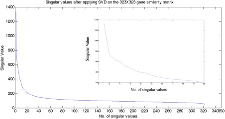
Singular Values after applying SVD on the braingene × gene matrix. It is observed that the singular values level off at around the 20th value. [Color figure can be viewed in the online issue, which is available at http://wileyonlinelibrary.com.]

Figure 2.

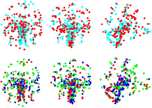
Effect of using SVD for dimensionality reduction on spectral clustering results. Clustering is done on the reduced correlation matrix constructed after applying SVD dimensionality reduction. It is observed that SVD fails to find distinct patterns in data, while using GDA for dimensionality reduction results in more distinct clusters (Figs. 3 and 4). The axial, coronal and sagittal views for two and three clusters are shown. [Color figure can be viewed in the online issue, which is available at http://wileyonlinelibrary.com.]

Because linear dimensionality reduction exhibited no discernible clustering tendency, nonlinear reduction was explored. After experimenting with various kernels, the Gaussian kernel of width σ = 1 was found to give the most stable clusters over repeated trials. Lower values of σ made the kernel too restricted in a higher dimensional space and higher values smoothed the data and curbed the method's ability to find nontrivial patterns. The clustering results of non‐linear dimensionality reduction via GDA with a Gaussian kernel of σ = 1, shown in Figure 3, demonstrate a clear spatial segregation. Typical of clustering techniques, our clustering results are consistent only about 80% of the time in repeated trials. To overcome the effect of initial seeding on the k‐means clustering algorithm, we implemented the majority vote rule. Cluster 1 (blue) represents the posterior/occipital/medial cortical group; cluster 2 (purple) represents the cerebellum/striatum/basal group; and cluster 3 (green) represents a frontal cortical group. The results for the other Microarray dataset are reproduced in Figure 4. Exploratory analysis was performed to test the influence of the kernel type and shape, as well as the selection of gene similarity measure; the results were similar to those shown here.

Figure 3.

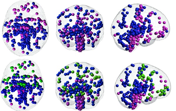
Spectral clustering of the gene correlation matrix for the first microarray expression dataset. GDA is applied to reduce the gene expression matrix and then Pearson's correlation is employed as a similarity measure. The axial, coronal and sagittal views are shown for 2 (top row) and 3 (bottom row) clusters. Brain regions that have a higher gene similarity are clustered together. The cluster shown in blue is consistent between groupings of two and three. Points belonging to the purple cluster in the top row split into two groups, represented by green and purple in the bottom row.

Figure 4.

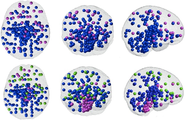
Spectral clustering of the gene correlation matrix for the second microarray expression dataset. GDA is applied to reduce the gene expression matrix and then Pearson's correlation is employed as a similarity measure. The axial, coronal and sagittal views are shown for 2 (top row) and 3 (bottom row) clusters. The high degree of similarity with the first data set (Fig. 3) is apparent. [Color figure can be viewed in the online issue, which is available at http://wileyonlinelibrary.com.]

Figure 5A shows the gene correlation matrices after using GDA (left) and SVD (right) for dimensionality reduction. There were obvious clusters present in the GDA matrix that are not as apparent in the SVD matrix, which was reflected in the clustering results in the previous section. In the GDA matrix, Cluster 1 (C1) represents the posterior/occipital/medial cortical group, cluster 2 (C2) represents the cerebellum/striatum/basal group and cluster 3 (C3) represents a frontal cortical group. Further clustering within the posterior/occipital/medial cortical group C1 shows 3 sub‐clusters CC1, CC2, and CC3 as displayed in Figure 5B. It is interesting to note that CC2, containing points in the cerebellum and the thalamus and displayed as red points in the C1 subcluster illustration, is also prominent in the SVD reduced correlation matrix. No discernible sub‐clusters were found for clusters 2 and 3.

Figure 5.

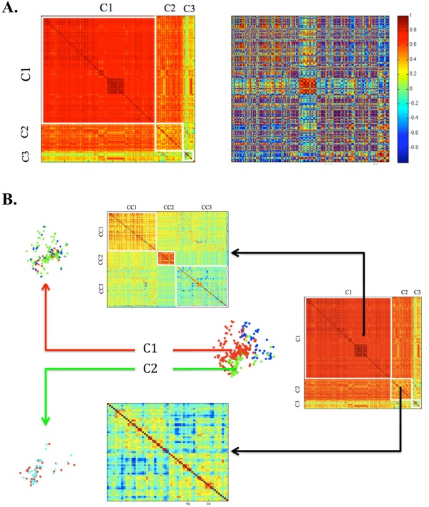
Gene correlation matrices after dimensionality reduction using GDA and SVD. (A) It can be inferred by looking at the correlation matrix after GDA (left) that a spectral clustering algorithm would give segregated clusters designated by C1, C2, and C3. However, the correlation matrix obtained after SVD (right) has no particular pattern except a red block in the center indicating a very high correlation between certain points, which is also observed in the GDA reduced correlation matrix. These gene points were found to belong to the cerebellum and the thalamus (B) Clustering was done considering C1, C2, and C3 individually to find sub‐clusters in the GDA reduced matrix. For C1, 3 subclusters were visible designated by CC1, CC2, and CC3. The corresponding gene points in the brain are shown on the left. Points shown in red (CC2) belong to the cerebellum and thalamus which according to this clustering result, share more gene expression compared to other gene points in the posterior/occipital/medial cortical cluster C1. However, clustering failed to segregate points within the cerebellum/striatum/basal group (C2) and the frontal cortical group (C3). [Color figure can be viewed in the online issue, which is available at http://wileyonlinelibrary.com.]

To determine the genes that may be responsible for spatial clustering, we took those with the most significant gene expression level differences between pairs of groups as measured by t tests between the three groups. Several genes which have functions like cell differentiation and morphogenesis appeared in the top 24 list. The gene list is shown in Table 1 with a clear designation of which pair of clusters the genes came from.

Table 1.

Gene list responsible for spatial clustering

S no.	Gene symbol	Description	Function	From paired t test between clusters
1.	CBLN2	Cerebellin 2 precursor	CBLN2 specific polypeptides serve as modulators of the endocrine system	1 and 2, 1 and 3
2.	TPPP3	Tubulin polymerization‐promoting protein family member 3	May play a role in cell proliferation and mitosis	1 and 2
3.	HGF	Hepatic Growth Factor	Acts as a growth factor for a broad spectrum of cell types	1 and 2
4.	BAIAP2L2	BAI1‐associated protein	Induces the formation of planar or gently curved membrane structures	1 and 2
5.	ADH7	Alcohol dehydrogenase 7	Could function in retinol oxidation for the synthesis of retinoic acid, a hormone important for cellular differentiation	1 and 2
6.	FAM110C	Family with sequence similarity 110, member C	May play a role in microtubule organization	1 and 2
7.	CDH12	Cadherin 12	Acts as a negative regulator of neural cell growth	1 and 3
8.	CDH13	Cadherin 13	Acts as a negative regulator of neural cell growth	1 and 3
9.	LGALS2	Lectin, galactoside‐binding,soluble 2	Binds beta‐galactoside. Its physiological function is not yet known	1 and 3
10.	GPR26	G protein‐coupled receptor 26	Orphan receptor. Displays a significant level of constitutive activity	1 and 3
11.	PFDN2	Prefoldin subunit 2	Binds to nascent polypepride chain and promotes folding in an environment	2 and 3
12.	CD63	CD63 molecule	The proteins mediate signal transduction events that play a role in the regulation of cell development, activation, growth and motility.	1 and 2
13.	PHIP	Pleckstrin Homology domain Interacting Protein	Probable regulator of the insulin and insulin‐like growth factor signaling pathways. Plays a role in the regulation of cell morphology and cytoskeletal organization	2 and 3
14.	H1FX	H1 histone family, member X	Histones H1 are necessary for the condensation of nucleosome chains into higher order structures	2 and 3
15.	SEMA4C		Required for normal brain development, axon guidance and cell migration (By similarity). Probable signaling receptor which may play a role in myogenic differentiation	2 and 3
16.	MY018A	Myosin XVIIIA	May be involved in the maintenance of the stromal cell architectures required for cell to cell contact	2 and 3
17.	NTS	Neurotensin		1 and 2
18.	ENC1	Ectodermal‐Neural Cortex 1	Actin‐binding protein involved in the regulation of neuronal process formation and in differentiation of neural crest cells. May be down‐regulated in neuroblastoma tumors
19.	SRGAP1	SLIT‐ROBO Rho GTPase activating protein 1	Together with CDC42 seems to be involved in the pathway mediating the repulsive signaling of Robo and Slit proteins in neuronal migration	1 and 2
20.	CAMK4	Calcium/Calmodulin‐Rdependent Protein Kinase IV	Phosphrylates the transcription activator CREB1 on 'Ser‐133' in hippocampal neuron nuclei and contribute to memory consolidation and Long Term Potentiation (LTP) in the hippocampus.	1 and 3
21.	TF	Transferrin	May have a role in stimulating cell proliferation	1 and 3
22.	PLP1	Proteolipid Protein 1	This is the major myelin protein from the Central Nervous System. It plays an important role in the formation and maintenance of the multilamellar structure of myelin	1 and 3
23.	MBP	Myelin Basic Protein	They are the most abundant protein components of the myelin membrane in the CNS. They have a role in both its formation and stabilization. The smaller isoforms might have an important role in remyelination of denuded axons in multiple sclerosis	1 and 3
24.	FTH1	Ferritin, heavy polypeptide 1	Defects in ferritin proteins are associated with several neurodegenerative diseases	1 and 3

A list of genes which might be responsible for spatial clustering indicating the clusters the genes came from. Cluster 1 represents the posterior/occipital/medial cortical group; cluster 2 represents the cerebellum/striatum/basal group; and cluster 3 represents a frontal cortical group.

Second Hypothesis: Anatomic Connectivity is Related to Gene Expression Similarity

First, we investigated correlations between pair‐wise structural connectivity (ACS) and similarity of gene expression profiles. The results, shown in (Fig. 6A) provided no evidence for significance at the level of pairwise connectivity. Next we tested whether the similarity of gene expression was significantly (negatively) correlated with the fiber distance between two regions. Fiber distance is defined here as the average length (in mm) of all fiber tracts going between the two regions as measured by whole brain tractography. Figure 6B illustrates a highly significant p‐value but a relatively weak R² likely due to the extremely large number of connections tested. Therefore, we concluded that again there is no evidence for this relationship. Finally, we tested whether gene similarity varies inversely with the geometric distance between gene sample points—here we directly used all 946 points and computed the distance (in mm) between them. The results, given in Figure 6C, again demonstrated weak evidence for this relationship.

Figure 6.

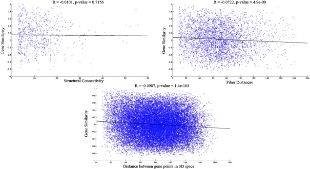
Scatter plots showing correlation coefficient and p‐values between gene similarity matrix and structural connectivity, fiber distance and Euclidean distance between gene points. (A) No correlation is found between the structural connectivity matrix obtained from tractography and the gene correlation matrix. (B) A negative correlation coefficient of 0.0722 with a significant p‐values = 0.001 <0.05 is found between the square matrix of fiber distances and the gene correlation matrix. (C) When the actual Euclidean distance between the gene points in 3D space is taken, a negative correlation of 0.0987 is found with the gene similarity matrix. However, small p‐values are probably occurring because of the large number of points in the comparison and hence these results may not indicate a true underlying relationship. [Color figure can be viewed in the online issue, which is available at http://wileyonlinelibrary.com.]

The objective of the statistical test as described in the Methods section was to prove that the error function $\delta (L,S)=\Vert {\widehat{\sigma }}^2{L}^{T}L-S^{-1}\Vert$ f was significantly smaller for the Laplacian of the actual connectivity matrix $L_0$, than for 10,000 other random matrices $L$. From Figure 7, it is clear that the value of the true discrepancy $\delta (L_0,S)$ is much lower than that of a large majority of equivalent models involving random matrices $L_k$. Figure 7A is the case when no filter is applied on the set of genes and cosine similarity of the gene points is used. Figure 7B,C show the histogram when the gene variance and the gene low‐value filters were used, retaining the top 10 percentile (left) and top 1‐percentile (right) genes, respectively. P values, representing the probability of type I error, obtained from each histogram are found to be significantly <0.05. Three of the five p‐values obtained from each histogram are <0.05 even after adjusting for multiple comparisons, thereby providing strong evidence for the gene‐connectivity hypothesis.

Figure 7.

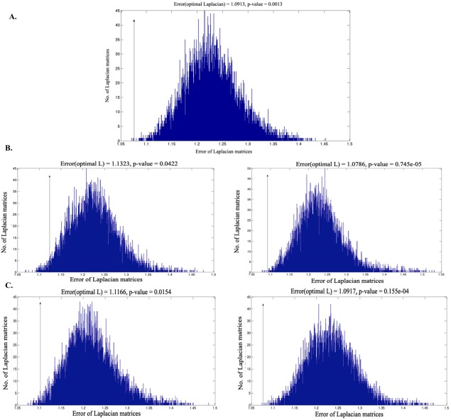
True matrix discrepancy δ(L₀, S) denoted with an arrow along with a histogram of the randomly generated matrix discrepancy δ(L, S). (A) No gene filtering. (B) Only the top 10 percentile and top 1 percentile genes with the highest variance are retained. (C) The top 10 percent and 1 percent genes with the highest absolute expression values are retained. [Color figure can be viewed in the online issue, which is available at http://wileyonlinelibrary.com.]

DISCUSSION

Comparison with Published Animal Data

Previously, many studies have compared gene expression atlases in the mouse brain and deduced inter‐regional differences in molecular signatures reflected by gene expression [Bohland et al., 2010; Chen et al., 2011; French and Pavlidis, 2011; French et al., 2011; Grange and Mitra, 2011; Lein et al., 2007; Sunkin and Hohmann, 2007; Wolf et al., 2011; Zapala et al., 2005], the earliest being on a nematode C. elegans [Kaufman et al., 2006]. The work in this nematode proved that the expression signature of a neuron carries significant information about its synaptic connectivity. There is evidence for both conserved genetic patterning mechanisms between rodents and humans as well as species‐specific differences [Chen et al., 2011]. In Bohland et al. [2010], clustering of voxels according to similarity of expression across a 3041 gene set was done to explore the spatial structure of gene expression patterns. In Hawrylycz et al. [2012], expression pattern clustering of 5000 prefiltered genes revealed similarity in regions like the striatum, cortex, hippocampus and smaller nuclei like the globus pallidus. In each of these studies, spatial location of gene expression appears to reflect anatomy, thus connecting knowledge at molecular level with higher‐level information about brain organization. Interestingly, similar clustering results were found when we used the similarity matrix based on only the human homologues of the 2000 mouse genes identified by ABI to be responsible for spatial organization in the mouse brain.

However, it is important to note that further subdivision of the cerebral cortex is not evident in any of these studies. Most authors have noted that neocortical gene expression patterns are relatively uniform across all cortical areas, although they vary considerably between laminae, suggesting that the canonical microcircuit is conserved across the cortex [Hawrylycz et al., 2012]. However, there is inconsistent evidence that functionally specific cortical regions, e.g. the somatosensory cortex, show enriched expression of specific genes.

Comparison with Published Human Data

Our results are consistent with a recent study by ABI [Hawrylycz et al., 2012], which correlated functional and genetic brain architecture, in several ways. No hemispheric differences are found in gene expression profiles in either study, with the neocortex displaying a relatively homogenous transcriptional pattern. Another approach to explore the spatial patterning of genetic information in the human brain was suggested on twin studies [Chen et al., 2011, 2012], where genetic patterning of cortical surface area revealed a bilaterally symmetric pattern of regionalization and an anterior–posterior division. Interestingly, their results mirror ours in the following ways: (1) the patterns identified in the left and right hemispheres were almost mirror images of one another, (2) they showed mixed effects of long‐distance anatomic connectivity on correlation patterns, and (3) they showed evidence for a hierarchical structure of genetic patterning [Chen et al., 2012]. It must be noted however, that these previous reports did not directly measure the spatial patterning of gene expression, what they investigated was the relationship of spatially distributed phenotypes on imaging metrics like cortical thickness and area. The observation that our results are broadly in agreement with those obtained from a very differently designed study provides a level of confidence in our results.

Hawrylycz et al. [2012] ask the question of how transcription varies across the neocortex and analyze genes underlying the function of specific brain regions. An online tool (WGCNA) is used to group genes with covarying expression patterns into modules and imputing eigengenes for each module. Our approach differs in that we do not preselect genes and we use a non‐linear dimensionality reduction method which, in conjunction with graph clustering, reveals three basic clusters in the neocortex. We also investigate genes which may be driving this clustering. Many of these genes are specifically geared for neuronal growth, differentiation and axonal guidance. The Cadherins (CDH12 and CDH13) are negative regulators of neural cell growth, PLP1 and MBP (Myelin Basic Protein) are specifically found in the CNS and play a role in formation and maintenance of myelin. SEMA4C is also known to play a role in normal brain development (http://www.genecards.org). HGF (hepatic growth factor) is responsible for growth of various cell types and of neurons, and TPPP3 for cell proliferation and mitosis. CBLN2, GPR26, and CAMK4 are found to be responsible for spatial clustering in the mouse brain [Kasukawa et al., 2011].

Except for the recent findings in [Hawrylycz et al., 2012], there is no comparable literature on gene clustering in the human brain. Human studies are hindered by challenging acquisition, limited tissue samples and, more importantly, because the architectonic, structural and molecular differences in the adult human neocortex are much more subtle than in animals [Hawrylycz et al., 2012; Lein et al., 2007]. This relative uniformity of expression within the neocortex has made it very difficult to obtain spatial clustering in humans.

Our clustering results indicate three regional groupings, largely conforming to known anatomic and functional boundaries. Evidence for further clustering is not present in our analysis. These results finally complete the circle from nematode to mouse to human, providing the same conclusion for each species. Although expression diversity conforms to architectonic and evolutionary differences between neocortex and older brain structures, there is now evidence that the neocortex is itself divided into primarily posterior/medial versus frontal structures.

Linear Versus Non‐linear Dimensionality Reduction

The linear approach (SVD) we used was successful in some prior studies on human genome microarray data, but only after manually selecting a very small subset of genes with known neurological relevance imputed from mouse data [Hawrylycz et al., 2012]. Given the differences between animal and human genomes and the possibility of biasing the analysis, we chose not to adopt this linear method; instead relying on our non‐linear dimensionality reduction method to uncover patterns buried in the entire genome. There is substantial evidence from machine learning literature [Fodor, 2002] that linear reduction is inadequate for large dimensions and complex interactions, where clusters may not be linearly separable. Usually these clusters lie on a manifold in feature space, and their separation becomes obvious only after “unrolling” the manifold. This is exactly what the presented non‐linear GDA method does. Besides avoiding manual intervention and providing a novel approach, using the non‐linear GDA method has the additional advantage of finding hitherto unknown genes that might be responsible for driving clustering. Our GDA results could propel new investigations of genomic data using this approach.

Comparison with Evolutionary/Embryological Evidence

The clustering groups that we found conform to previous animal studies, making our results the human analogue of reported caudal‐rostral clustering along the neural tube in animals. A recent study [Zapala et al., 2005] suggests that the adult mouse brain bears a transcriptional “imprint” reflecting embryological and evolutionary relationships between brain regions. Embryonic cellular position along the anterior–posterior axis of the neural tube was shown to be closely associated with gene expression patterns of adult brain structures. Gene expression clustering analysis revealed a hierarchical organization whereby the telencephalon, the diencephalon and the mesencephalon form gene‐expression based clusters. Furthermore, weak clustering of telencephalon into evolutionarily progressive regions (archicortex, paleocortex, and neocortex) was also found. Interestingly, the result shown here in human brains is similar to this observation on mouse brains. The three main spatial clusters we found are also organized along the caudal‐rostral neural axis, and represent the classic hindbrain‐midbrain‐forebrain evolutionary paradigm. We found some structures cluster more with their embryological/evolutionary groupings rather than by proximity or function. For instance, the Globus Pallidus and Substantia Nigra are grouped into different clusters, in keeping with their evolutionary origins—telencephalon versus mesencephelon, respectively—even though they are close both anatomically and functionally [Kasukawa et al., 2011]. This concordance with animal studies represents the most likely source of molecular diversity seen in the brain of any mammalian species: architectonic diversity arising from embryogenic and evolutionarily‐guided cell differentiation and specialization.

The Gene–Connectivity Relationship

The analysis presented in Figures 5 and 6 addresses a connectionist hypothesis, which posits that observed diversity of genetic expression in the brain might simply be a result or cause of structural connectivity between like species [Brodmann, 1909]. How can such connectivity come about? There exists a direct and well‐known correspondence between cytoarchitecturally defined brain regions and the inherent connectivity within them [Zilles and Amunts, 2010]. The visual, sensorimotor and limbic systems, for example, display expression heterogeneity from other regions in that they are connected in a manner different from the rest of the cortex. The so‐called default mode network possessed different cytoarchitectural attributes from other cortices [Greicius et al., 2003; Harrison et al., 2008]. The action of neurotransmitters is regionally dependent [Johnson et al., 2009] and the effect of neurotrophic factors ensures that connections between certain matched neurotrophin/receptor pairs survive in preference to non‐matched pairs [Ebendal, 1992; Heerssen and Segal, 2002; Skaper, 2012; Wetmore and Olson, 1995]. BDNF pairs specifically with trkB, and NGF with trkA [Skaper, 2012]. The totality of these observations suggests that there should be some molecular‐cellular correlate of structural connectivity, that is, connectivity between “like” or matched regions with similar population of cell types should enervate each other more often than non‐matched or unlike regions.

A small number of animal studies have considered this problem. In [French et al., 2011], the authors identify spatial correlations between gene expression and connectivity using the expression energy to rank genes according to Spearman correlation coefficient using only pairs with the strongest correlation for further analysis. Two new patterns of mouse brain gene expression were identified which reflect regional differences in cellular populations. In [French and Pavlidis, 2011], 17,530 genes in a 142 anatomical region atlas were used to show that gene expression signatures have a statistically significant relationship with connectivity between neurons. A similar analysis on selected neurotrophins and their receptors in [Lohof et al., 1993; Scott and Luo, 2001] suggests a correlation between connectivity and molecular similarity.

Although these studies have satisfactorily shown correlation, they are unable to determine whether observed molecular signatures are purely, mainly or partially a determinant of connectivity. This presents an important but overlooked issue: does the observed gene expression diversity arise from regional predilections resulting from embryogenic or evolutionary progression, or is it a simple consequence of the brain's “connectomics”? If both effects are present, which one dominates? Can the spatially distinct clustering of gene expression data we found be explained solely as an effect of networking between like‐species neurons? Human twin studies [Rimol et al., 2010] found high genetic correlations between homologous areas in opposite hemispheres, which cannot generally be explained by direct connections. Yet another twin study found evidence of long‐range genetic correlations mediated by anatomic connectivity [Chen et al., 2011]; for instance fronto‐temporal correlations were thought to be mediated by the Uncinate Fasciculus.

Likewise, the evidence from our results (Figs. 5 and 6) is mixed. Taken together, our results indicate that neither connectivity nor geometric distance determines gene diversity, and vice versa. We found no evidence that structural connectivity determines gene similarity. Although previous reports described above have demonstrated correlations in isolated region pairs, we concluded that it is not optimal to consider pairwise relationships because the brain connectivity network is a large‐scale, complex network. Even if a significant relationship existed between connectivity and gene expression, it is unlikely to be revealed by considering regions pairs separately. Instead, we need to consider the effect of the entire pattern of gene expression on whole brain connectivity. Because we found no published accounts of how to do this, we designed a novel whole brain connectivity formulation for testing this hypothesis. This latter, somewhat unconventional, analysis in which we assume a direct relationship between connectivity and gene similarity, was successful. On the basis of the statistical test we set up for our hypothesis, we concluded that although no inter‐regional connection is determined solely by gene similarity between them, the overall connectivity network conforms to inter‐regional gene similarity data in a way that cannot arise by chance. Thus, gene expression influences rather than determines structural connectivity.

Limitations and Future Work

Although our clustering and connectivity results appear robust and insensitive to parameter choice, they exhibit some sensitivity to the choice of anatomic atlas used for combining neighboring sample points. This may be due to the difference in methods used for regional dissections [Johnson et al., 2009]. A related limitation is our use of different brain parcellations for addressing the two hypotheses. The first hypothesis needed the sampled gene points to be combined by tissue type, into 323 regions according to the histopathological labels provided by the ABI. The second hypothesis required structural connectivity information, and for this we chose to begin with the MNI brain atlas parcellations used and tested in our previous connectivity work [Kuceyeski et al., 2011]. This atlas was subdivided into roughly equal anatomically and functionally cohesive regions, which by virtue of being grandfathered by an existing and widely used parcellation, would provide comparable connectomes. Because the ABA gene sample locations were not chosen with connectivity in mind, the ABA‐derived atlas used in Hypothesis 1 would not be well suited for Hypothesis 2. For example, the density of sampling in ABA is highly variable across the brain; taking extremely small regions as nodes is unreliable due to noise and problems in tractography [Ivković et al., 2012; Kuceyeski et al., 2011].

Another disadvantage of our work is the availability of only two subjects' gene expression profiles from the ABI at the time of writing. Although we have demonstrated high consistency between the two brains available from ABI, the absence of multiple subjects precludes filtering out outliers, inconsistent or divergent expression levels, and random and systematic noise arising from microarray analysis [Brody et al., 2002; Brown et al., 2001]. Microarray data has limited spatial resolution and accuracy compared to histopathological measurements. Another source of error could be in the connectivity matrix C used for hypothesis 2. This matrix is obtained using probabilistic tractography [Kuceyeski et al., 2011] which suffers from the inability to resolve long‐range fibers.

A possibility we did not investigate in this work is that gene expression similarity could be revealed by “chemical” connectivity via the distinct domains of various neurotransmitters and neurotrophic factors. Already we can see this in our clustering results: dopaminergic circuits in the brainstem and basal ganglia appear to be clustered together, and initial investigations into genes coding for neurotrophic factors also showed stereotyped spatial patterns. This is a very important and large new question, which will require careful and detailed work, currently underway in our laboratory.

REFERENCES

- Alemán‐Gómez Y, Melie‐García L, Valdés‐Hernandez P (2006): IBASPM: Toolbox for automatic parcellation of brain structures. Available on CD‐Rom in NeuroImage 31(Suppl 1). Available at http://www.thomaskoenig.ch/Lester/ibaspm.htm.
- Alter O, Brown PO, Botstein D (2000): Singular value decomposition for genome‐wide expression data processing and modeling. Proc Natl Acad Sci USA 97:10101–10106. [DOI] [PMC free article] [PubMed] [Google Scholar]
- Auffarth B (2007): Spectral graph clustering. Universitat de Barcelona, course report for Technicas Avanzadas de Aprendizaj, at Universitat Politecnica de Catalunya.
- Bernard A, Lubbers LS, Tanis KQ, Luo R, Podtelezhnikov AA, Finney EM, McWhorter MME, Serikawa K, Lemon T, Morgan R, Copeland C, Smith K, Cullen V, Davis‐Turak J, Lee CK, Sunkin SM, Loboda AP, Levine DM, Stone DJ, Hawrylycz MJ, Roberts CJ, Jones AR, Geschwind DH, Lein ES, (2012): Transcriptional architecture of the primate neocortex. Neuron 73:1083–1099. [DOI] [PMC free article] [PubMed] [Google Scholar]
- Bohland JW, Bokil H, Pathak SD, Lee C‐K, Ng L, Lau C, Kuan C, Hawrylycz M, Mitra PP (2010). Clustering of spatial gene expression patterns in the mouse brain and comparison with classical neuroanatomy. Methods (San Diego, CA) 50:105–512. [DOI] [PubMed] [Google Scholar]
- Brodmann K (1909): Vergleichende Lokalisationslehre der Gro hirnrinde. Notes.
- Brody JP, Williams BA, Wold BJ, Quake SR (2002): Significance and statistical errors in the analysis of DNA microarray data. Proc Natl Acad Sci USA 99:12975–12978. [DOI] [PMC free article] [PubMed] [Google Scholar]
- Brown CS, Goodwin PC, Sorger PK (2001): Image metrics in the statistical analysis of DNA microarray data. Proc Natl Acad Sci USA 98:8944–8949. [DOI] [PMC free article] [PubMed] [Google Scholar]
- Chen C‐H, Panizzon MS, Eyler LT, Jernigan TL, Thompson W, Fennema‐Notestine C, Jak AJ, Neale MC, Franz CE, Hamza S, Lyons MJ, Grant MD, Fischl B, Seidman LJ, Tsuang MT, Kremen WS, Dale AM (2011): Genetic influences on cortical regionalization in the human brain. Neuron 72:537–544. [DOI] [PMC free article] [PubMed] [Google Scholar]
- Chen C‐H, Gutierrez ED, Thompson W, Panizzon MS, Jernigan TL, Eyler LT, Fennema‐Notestine C, Dale AM (2012): Hierarchical genetic organization of human cortical surface area. Science (New York, NY) 335:1634–1636. [DOI] [PMC free article] [PubMed] [Google Scholar]
- Ebendal T (1992): Function and evolution in the NGF family and its receptors. J Neurosci Res 32:461–470. [DOI] [PubMed] [Google Scholar]
- Fisher R (1936): The use of multiple measurements in taxonomic problems. Ann Hum Genet 7:179–188. [Google Scholar]
- Fodor IK (2002): A survey of dimension reduction techniques. LLNL Technical Report, UCRL‐ID‐148494:1–18.
- French L, Pavlidis P (2011): Relationships between gene expression and brain wiring in the adult rodent brain. PLoS Comput Biol 7:e1001049. [DOI] [PMC free article] [PubMed] [Google Scholar]
- French L, Patrick P, Tan C, Pavlidis P, Wolf L (2011): Large‐scale analysis of gene expression and connectivity in the rodent brain: Insights through data integration. Gene Expression 5:1–11. [DOI] [PMC free article] [PubMed] [Google Scholar]
- Friston KJ, Ashburner JT, Kiebel SJ, Nichols TE, Penny WD (2006): Statistical parametric mapping: the analysis of functional brain images. Friston, K 454–470.
- Grange P, Mitra PP (2011): Statistical analysis of co‐expression properties of sets of genes in the mouse brain arXiv preprint arXiv:1111.6200 .
- Greicius MD, Krasnow B, Reiss AL, Menon V (2003): Functional connectivity in the resting brain: A network analysis of the default mode hypothesis. Proc Natl Acad Sci USA 100:253–258. [DOI] [PMC free article] [PubMed] [Google Scholar]
- Harrison BJ, Pujol J, López‐Solà M, Hernández‐Ribas R, Deus J, Ortiz H, Soriano‐Mas C, Yusel M, Pantelis C, Cardoner N, (2008): Consistency and functional specialization in the default mode brain network. Proc Natl Acad Sci USA 105:9781–9786. [DOI] [PMC free article] [PubMed] [Google Scholar]
- Hawrylycz MJ, Lein ES, Guillozet‐Bongaarts AL, Shen EH, Ng L, Miller JA, Van de Lagemaat LN, et al. (2012): An anatomically comprehensive atlas of the adult human brain transcriptome. Nature 489:391–399. [DOI] [PMC free article] [PubMed] [Google Scholar]
- Heerssen HM, Segal RA (2002): Location, location, location: A spatial view of neurotrophin signal transduction. Trends Neurosci 25:160–165. [DOI] [PubMed] [Google Scholar]
- Iturria‐Medina Y, Canales‐Rodriguez EJ, Aleman‐Gomez Y, Sotero RC, Melie‐Garcia L (2005): Bayesian formulation for fiber tracking. 11th Annual Meeting of the Organization for Human Brain Mapping (Toronto, Ontario, Canada) . 26.
- Iturria‐Medina Y, Canales‐Rodriguez EJ, Aleman‐Gomez Y, Sotero RC, Melie‐Garcia L (2008): Studying the human brain anatomical network via diffusion‐weighted MRI and graph theory. NeuroImage 40:1064–1076. [DOI] [PubMed] [Google Scholar]
- Ivković M, Kuceyeski A, Raj A (2012): Statistics of weighted brain networks reveal hierarchical organization and gaussian degree distribution. PloS One 7:e35029. [DOI] [PMC free article] [PubMed] [Google Scholar]
- Johnson MB, Kawasawa YI, Mason CE, Krsnik Z, Coppola G, Bogdanović D, Geschwind DH, Mane SM, State MW, Sestan N (2009): Functional and evolutionary insights into human brain development through global transcriptome analysis. Neuron 62:494–509. [DOI] [PMC free article] [PubMed] [Google Scholar]
- Jones AR, Overly CC, Sunkin SM (2009): The allen brain atlas: 5 years and beyond. Nat Rev Neurosci 10:821–828. [DOI] [PubMed] [Google Scholar]
- Kasukawa T, Masumoto K‐H, Nikaido I, Nagano M, Uno KD, Tsujino K, Hanashima C, Shigeyoshi Y, Ueda HR (2011): Quantitative expression profile of distinct functional regions in the adult mouse brain. PloS One 6:e23228 Available at: http://www.pubmedcentral.nih.gov/articlerender.fcgi?artid=3155528&tool=pmcentrez&rendertype=abstract. [DOI] [PMC free article] [PubMed] [Google Scholar]
- Kaufman A, Dror G, Meilijson I, Ruppin E (2006): Gene expression of Caenorhabditis elegans neurons carries information on their synaptic connectivity. PLoS Comput Biol 2:e167. [DOI] [PMC free article] [PubMed] [Google Scholar]
- Krzanowskit W (1995): Discriminant analysis with singular covariate matrices: Methods and applications to spectroscopic data. Appl Stat 44:101–115. [Google Scholar]
- Kuceyeski A, Maruta J, Niogi SN, Ghajar J, Raj A (2011): The generation and validation of white matter connectivity importance maps. NeuroImage 58:109–121. Available at: http://www.pubmedcentral.nih.gov/articlerender.fcgi?artid=3144270&tool=pmcentrez&rendertype=abstract. [DOI] [PMC free article] [PubMed] [Google Scholar]
- Lein ES, Hawrylycz MJ, Ao N, Ayres M, Bensinger A, Bernard A, Boe AF, Boguski MS, Brockway KS, Byrnes EJ, Chen L, Chen L, Chen TM, Chin MC, Chong J, Crook BE, Czaplinska A, Dang CN, Datta S, Dee NR, et al. (2007): Genome‐wide atlas of gene expression in the adult mouse brain. Nature 445:168–176. [DOI] [PubMed] [Google Scholar]
- Lohof Ann M, Nancy Y, Mu‐Ming P (1993): Potentiation of developing neuromuscular synapses by the neurotrophins NT‐3 and BDNF. Nature 363:350–353. [DOI] [PubMed] [Google Scholar]
- Ng AM, Jordan YW, Weiss Y, (2002): On spectral clustering: analysis and an algorithm. Advances in Neural Information Processing Systems 14:849–856. [Google Scholar]
- Rimol LM, Panizzon MS, Fennema‐Notestine C, Eyler LT, Fischl B, Franz CE, Hagler DJ, Lyons MJ, Neale MC, Pacheco J, Perry ME, Schmitt JE, Grant MD, Seidman LJ, Thermenos HW, Tsuang MT, Eisen SA, Kremen WS, Dale AM (2010): Cortical thickness is influenced by regionally specific genetic factors. Biol Psychiatry 67:493–499. [DOI] [PMC free article] [PubMed] [Google Scholar]
- Russo G, Zegar C, Giordano A (2003): Advantages and limitations of microarray technology in human cancer. Oncogene 22:6497–6507. [DOI] [PubMed] [Google Scholar]
- Schaeffer SE (2007): Graph clustering. Comp Sci Rev 1:27–64. [Google Scholar]
- Schena M, Shalon D, Davis RW, Brown PO (1995): Quantitative monitoring of gene expression patterns with a complementary DNA microarray Science (New York, N.Y.) 270:467–470. [DOI] [PubMed] [Google Scholar]
- Scott EK, Luo L (2001): How do dendrites take their shape? Nat Neurosci 4:359–365. [DOI] [PubMed] [Google Scholar]
- Shalon D, Smith SJ, Brown PO (1996): A DNA microarray system for analyzing complex DNA samples using two‐color fluorescent probe hybridization. Genome Res 6:639–645. [DOI] [PubMed] [Google Scholar]
- Singh S, Silakari S (2009): Generalized discriminant analysis algorithm for feature reduction in cyber. J Comp Sci 6:173–180. [Google Scholar]
- Skaper SD (2012): The neurotrophin family of neurotrophic factors: an overview. Methods Mol Biol 846:1–12. [DOI] [PubMed] [Google Scholar]
- Smola AJ, Kondor R (2003): Kernels and regularization on graphs. Learning theory and kernel machines (Springer Berlin Heidelberg). 144–158.
- Sunkin SM, Hohmann JG (2007): Insights from spatially mapped gene expression in the mouse brain. Hum Mol Genet 16:R209–R219. [DOI] [PubMed] [Google Scholar]
- Swanson LW (2000): What is the brain? Trends Neurosci 23:519–527. [DOI] [PubMed] [Google Scholar]
- Tzourio‐Mazoyer N, Landeau B, Papathanassiou D, Crivello F, Etard O, Delcroix N, Mazoyer B, Joliot M (2002): Automated anatomical labeling of activations in SPM using a macroscopic anatomical parcellation of the MNI MRI single‐subject brain. NeuroImage 15:273–289. [DOI] [PubMed] [Google Scholar]
- Wetmore C, Olson L (1995): Neuronal and nonneuronal expression of neurotrophins and their receptors in sensory and sympathetic ganglia suggest new intercellular trophic interactions. J Comp Neurol 353:143–159. [DOI] [PubMed] [Google Scholar]
- Wolf L, Goldberg C, Manor N, Sharan R, Ruppin E (2011): Gene expression in the rodent brain is associated with its regional connectivity. PLoS Comput Biol 7:e1002040. [DOI] [PMC free article] [PubMed] [Google Scholar]
- Ye J (2005): Characterization of a family of algorithms for generalized discriminant analysis on undersampled problems. J Machine Learn Res 6:483–502. [Google Scholar]
- Zapala MA, Hovatta I, Ellison JA, Wodicka L, Del Rio JA, Tennant R, Tynan W, Broide RS, Helton R, Stoveken BS, Winrow C, Lockhart DJ, Reilly JF, Young WG, Bloom FE, Lockhart DJ, Barlow C. (2005): Adult mouse brain gene expression patterns bear an embryologic imprint. Proc Natl Acad Sci USA 102:10357–10362. [DOI] [PMC free article] [PubMed] [Google Scholar]
- Zilles K, Amunts K (2010): Centenary of Brodmann's map—Conception and fate. Nat Rev Neurosci 11:139–145. [DOI] [PubMed] [Google Scholar]