Massive-Training Artificial Neural Network Coupled With Laplacian-Eigenfunction-Based Dimensionality Reduction for Computer-Aided Detection of Polyps in CT Colonography

Abstract

A major challenge in the current computer-aided detection (CAD) of polyps in CT colonography (CTC) is to reduce the number of false-positive (FP) detections while maintaining a high sensitivity level. A pattern-recognition technique based on the use of an artificial neural network (ANN) as a filter, which is called a massive-training ANN (MTANN), has been developed recently for this purpose. The MTANN is trained with a massive number of subvolumes extracted from input volumes together with the teaching volumes containing the distribution for the “likelihood of being a polyp;” hence the term “massive training.” Because of the large number of subvolumes and the high dimensionality of voxels in each input subvolume, the training of an MTANN is time-consuming. In order to solve this time issue and make an MTANN work more efficiently, we propose here a dimension reduction method for an MTANN by using Laplacian eigenfunctions (LAPs), denoted as LAP-MTANN. Instead of input voxels, the LAP-MTANN uses the dependence structures of input voxels to compute the selected LAPs of the input voxels from each input subvolume and thus reduces the dimensions of the input vector to the MTANN. Our database consisted of 246 CTC datasets obtained from 123 patients, each of whom was scanned in both supine and prone positions. Seventeen patients had 29 polyps, 15 of which were 5–9 mm and 14 were 10–25 mm in size. We divided our database into a training set and a test set. The training set included 10 polyps in 10 patients and 20 negative patients. The test set had 93 patients including 19 polyps in seven patients and 86 negative patients. To investigate the basic properties of a LAP-MTANN, we trained the LAP-MTANN with actual polyps and a single source of FPs, which were rectal tubes. We applied the trained LAP-MTANN to simulated polyps and rectal tubes. The results showed that the performance of LAP-MTANNs with 20 LAPs was advantageous over that of the original MTANN with 171 inputs. To test the feasibility of the LAP-MTANN, we compared the LAP-MTANN with the original MTANN in the distinction between actual polyps and various types of FPs. The original MTANN yielded a 95% (18/19) by-polyp sensitivity at an FP rate of 3.6 (338/93) per patient, whereas the LAP-MTANN achieved a comparable performance, i.e., an FP rate of 3.9 (367/93) per patient at the same sensitivity level. With the use of the dimension reduction architecture, the time required for training was reduced from 38 h to 4 h. The classification performance in terms of the area under the receiver-operating-characteristic curve of the LAP-MTANN (0.84) was slightly higher than that of the original MTANN (0.82) with no statistically significant difference (p-value).

I. Introduction

Colorectal cancer is the second leading cause of cancer deaths in the United States. Early detection and removal of polyps (the precursors of colorectal cancers) is a promising strategy for enhancing patients’ chance of survival. CT colonography (CTC) is an emerging technique for mass screening of colorectal carcinoma. The diagnostic performance of CTC in detecting polyps, however, remains uncertain because of a propensity for perceptual errors and substantial variations among readers in different studies. Computer-aided detection (CAD) of polyps has the potential to overcome these difficulties with CTC. CAD provides for radiologists the locations of suspicious polyps for their review, thus improving the diagnostic performance in the detection of polyps.

Automated detection of polyps with CAD schemes is a very challenging task, because the polyps have large variations in shapes and sizes and there are numerous colon folds and residual leftover colonic materials on the colon wall that mimic polyps. A number of researchers have recently developed automated or semi-automated CAD schemes in CTC. Although the performance of current CAD schemes has demonstrated a great potential, some limitations remain. One of the major limitations is a relatively large number of false-positive (FP) detections, which is likely to confound the radiologists’ image interpretation task and thus lower their efficiency. A large of number of FPs could adversely affect the clinical application of CAD for colorectal cancer screening. Therefore, methods for removal of computer FPs are in strong demand.

The common sources of FPs are haustral folds, residual stool, rectal tubes, and extra-colonic structures such as the small bowel and stomach, as reported in [1], [2]. Various methods have been proposed for the reduction of FPs, with variable success. Summers et al. [3], [4] employed the geometric features on the inner surface of the colon wall, such as the mean, Gaussian, and principal curvatures, to find polyp candidates. Yoshida et al. [5] and Näppi et al. [6] further characterized the curvature measures by using a shape index and curvedness to distinguish polyp candidates from the normal tissues of the colon wall. Paik et al. [7] and Kiss et al. [8] presented another solution for polyp detection in which they utilized the normal vector (rather than the curvature) and sphere fitting as references to extract some geometric features on the polyp surfaces. Because these traditional surface shape-based descriptions are sensitive to the irregularity of the colon wall, these CAD methods share a relatively high FP rate. Gokturk et al. [9] developed a scheme based on statistical pattern recognition, and they applied a 3-D pattern-processing method to the reduction of FPs. Acar et al. [10] used edge-displacement fields to model the changes in consecutive cross-sectional views of CTC data, as well as quadratic discriminant analysis. Jerebko et al. [11], [12] used a standard ANN to classify polyp candidates and improved the performance by incorporating a committee of ANNs and a committee of support vector machines. Yao et al. [13] explored image segmentation methods to reduce FPs. Iordanescu and Summers [14] developed an image-segmentation-based approach for the reduction of FPs due to rectal tubes.

The performance of a CAD scheme usually involves a trade-off between sensitivity and specificity. It is important to remove as many types of FPs as possible, while the sensitivity of a CAD scheme is maintained. For addressing this issue, a 3-D massive-training artificial neural network (MTANN) and a mixture of expert 3-D MTANNs were developed for elimination of a single type of FP [1] and multiple types of FPs [2], respectively. The mixture of expert 3-D MTANNs consists of several expert 3-D MTANNs in parallel, each of which is trained independently by use of a specific type of non-polyp and a common set of various types of polyps. Each expert MTANN acts as an expert for distinguishing polyps from a specific type of non-polyp. It was demonstrated in [15] that this mixture of expert MTANNs was able to eliminate various types of FPs at a high sensitivity level.

The training of an MTANN is, however, very time-consuming, [1], [2], [15]–[19]. For example, the training of a 3-D MTANN with ten polyps and ten FPs may take 38 h on a workstation [1], [2]. The training time will increase when the number of training cases increases. To address this time issue and make an MTANN work more efficiently, we propose here an MTANN coupled with a Laplacian-eigenfunction-based dimension reduction. In the MTANN framework, the input features are the large number of neighboring voxel values in each subvolume extracted from a CTC volume, and thus they have some underlying geometric structures and are highly dependent each other. Motivated by this fact, we employ a manifold-based dimension-reduction technique, a Laplacian eigenfunction [20], to improve the efficiency of the original MTANN. This will be demonstrated by use of both simulation and actual clinical data. Other nonlinear dimension reduction techniques such as the diffusion map [21] and Isomap [22] would have comparable results because they can take the local geometry information fairly well, whereas the classical principal-component analysis (PCA) is known for being sensitive to outliers and cannot incorporate the local intrinsic structure.

The paper is organized as follows. In Section II, we first describe our CTC database and review the basics of an MTANN, and we then explain the technical details for improvement by using Laplacian eigenfunctions. In Section III, we compare the results of the application of MTANNs with and without LAPs in experiments with both simulated and actual polyps. Finally, we further discuss the statistical issues of employment of LAPs in Section IV and give a conclusion in Section V.

II. Materials and Methods

A. Database

The database used in this study consisted of 246 CTC datasets obtained from 123 patients acquired at the University of Chicago Medical Center. Each patient was scanned in both supine and prone positions with a multi-detector-row CT scanner (LightSpeed QX/i, GE Medical Systems, Milwaukee, WI) with collimations between 2.5 and 5.0 mm, reconstruction intervals of 1.25–5.0 mm, and tube currents of 60–120 mA with 120 kVp. Each reconstructed CT section had a matrix size of 512 × 512 pixels, with an in-plane pixel size of 0.5–0.7 mm. In this study, we used 5 mm as the lower limit on the clinically significant size of polyps. Seventeen patients had 29 colonoscopy-confirmed polyps, 15 of which were 5–9 mm and 14 were 10–25 mm in size. We divided our database into a training set and a test set. The training set contained 10 polyps in 10 patients and 20 negative patients. The test set included 93 patients containing 19 polyps in 7 patients and 86 negative patients. We applied an initial CAD scheme for detection of polyps in CTC to our CTC database. The initial polyp-detection scheme is a standard CAD approach which consists of 1) colon segmentation based on CT value-based analysis and colon tracing [23], 2) detection of polyp candidates based on morphologic analysis of the segmented colon [5] followed by connected-component analysis [24]–[26], 3) calculation of 3-D pattern features of the polyp candidates [6], [27], [28], and 4) quadratic discriminant analysis [29] for classification of the polyp candidates as polyps or non-polyps based on the pattern features. The initial CAD scheme yielded a 95% (18/19) by-polyp sensitivity with 5.1 (474/93) FPs per patient for the test set. The major sources of FPs included rectal tubes, stool, haustral folds, colonic walls, and the ileocecal valve. These CAD detections were used for experiments for evaluating the performance of 3-D MTANNs.

B. Basics of an MTANN Framework

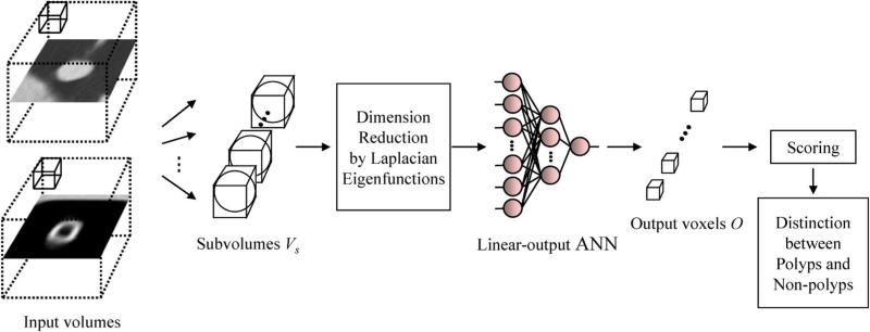
Supervised nonlinear image-processing techniques based on artificial neural networks (ANNs), called “neural filters” [30] and “neural edge enhancers” [31] were developed for reduction of the quantum mottle in X-ray images and for supervised detection of subjective edges traced by cardiologists [32], respectively. The neural filters and neural edge enhancers were extended to accommodate various pattern-classification tasks, and a 2-D MTANN was developed [15]. A 2-D MTANN was originally developed for distinguishing a specific opacity from other opacities in thoracic CT [15]. The 2-D MTANN was applied to the reduction of FPs in the computerized detection of lung nodules in chest radiography [17], low-dose CT [15], [18], and the suppression of ribs in chest radiographs [16]. A 3-D MTANN was recently developed for processing 3-D volume data in CTC [1], [2]. The architecture of a 3-D MTANN is shown in Fig. 1. A 3-D MTANN consists of a linear-output multilayer ANN model for regression, which is capable of operating on voxel data directly [31], [32]. The linear-output multilayer ANN model employs a linear function instead of a sigmoid function as the activation function of the unit in the output layer because the characteristics of an ANN were improved significantly with a linear function when applied to the continuous mapping of values in image processing [31]. Note that the activation functions of the units in the hidden layer are a sigmoid function for nonlinear processing, and those of the unit in the input layer are an identity function, as usual. The 3-D MTANN is trained with input CTC volumes and the corresponding teaching volumes for enhancement of polyps and suppression of non-polyps. The input to the expert 3-D MTANN consists of a collection of voxel values in a subvolume, V_s, extracted from an input volume, denoted as a vector $\mathbf{I}=(I^1,\dots ,I^n)\in {\Re }^n$, where each I_i denotes one input voxel in V_s. Here, n is the number of voxels in a sub-volume of a fixed size. The pixel values of the original CTC images are normalized first such that − 1000 HU (Hounsfield units) is zero and 1000 HU is one. The output of an MTANN is a continuous scalar value, which corresponds to the center voxel (p = 0, q = 0, r = 0)in the subvolume, V_s. The output at (x, y, z)is denoted by

$$O(x,y,z)=NN\{I(x-p,y-q,z-r)\mid (p,q,r)\in V_s\},$$ (1)

The entire output volume is obtained by scanning of the input subvolume of the MTANN on the entire input CTC volume. The input subvolume and the scanning of the MTANN can be analogous to the kernel of a convolution filter and the convolutional operation of the filter, respectively. Note that only one unit is employed in the output layer.

Fig. 1.

Architecture of a LAP-MTANN consisting of a massive-subvolume training scheme, dimension reduction by Laplacian eigenfunctions, and a linear-output ANN model. The input CTC volumes including a polyp or a non-polyp are divided voxel by voxel into a large number of overlapping 3-D subvolumes. Instead of all voxel values in each subvolume, only the top n Laplacian eigenfunctions of them are entered as an input vector to the linear-output ANN.

The teaching volume for polyps contains a 3-D Gaussian distribution with standard deviation σ_T, which approximates the average shape of polyps, and that for non-polyps contains only zeros. This distribution represents the likelihood of being a polyp

$$T(x,y,z)=\{\begin{array}{cc}\frac{1}{\sqrt{2\pi }{\sigma }_T}{e}^{-\frac{x^2+y^2+z^2}{2{\sigma }_T^2}}\hfill & \text{for a polyp}\hfill \\ 0\hfill & \text{for non}-\text{polyps}.\hfill \end{array}\phantom{\}}$$ (2)

For enrichment of the training samples, a massive number of overlapping subvolumes are extracted from a training volume V_T, and the same number of single voxels are extracted from the corresponding teaching volume as teaching values. The centers of consecutive subvolumes differ by just one pixel. All pixel values in each of the subvolumes may be entered as input to the 3-D MTANN, whereas one pixel from the teaching image is entered into the output unit in the 3-D MTANN as the teaching value. The error to be minimized in training is given by

$$E=\frac{1}{P}\sum _i\sum _{(x,y,z)\in V_T}{(T_i(x,y,z)-O_i(x,y,z))}^2$$ (3)

where i is a training case number, O_i is the output of the MTANN for the th case, T_i is the teaching value for the ith case, and P is the total number of training voxels in the training volume. The MTANN is trained by a linear-output back-propagation algorithm [31], [32] which was derived for the linear-output ANN model by use of the generalized delta rule [33].

After training, the MTANN is expected to output the highest value when a polyp is located at the center of the subvolume, a lower value as the distance from the subvolume center increases, and approximately zero when the input subvolume contains a non-polyp. The entire output volume is obtained by scanning of the whole input CTC volume to the MTANN. For the distinction between polyps and non-polyps, a 3-D scoring method based on the output volume of the trained MTANN is applied. A score for a polyp candidate is defined as

$$S=\sum _{(x,y,z)\in V_E}{f}_G(x,y,z;\sigma )\times O(x,y,z)$$ (4)

where

$$f_G(x,y,z;\sigma )=\frac{1}{\sqrt{2\pi }\sigma }{e}^{-\frac{x^2+y^2+z^2}{2{\sigma }^2}}$$ (5)

is a 3-D Gaussian weighting function with standard deviation σ with its center corresponding to the center of the volume for evaluation, V_E ; V_E is the volume for evaluation, which is sufficiently large to cover a polyp or a non-polyp; and O(x, y, z)is the output of the trained MTANN. The use of the 3-D scoring method allows us to combine the individual voxel-based responses (outputs) of a trained 3-D MTANN as a single score for each candidate. The score is the weighted sum of the estimates of the likelihood that a polyp candidate volume contains an actual polyp near the center, that is, a high score would indicate a polyp and a low score would indicate a non-polyp. The same 3-D Gaussian weighting function is used as in the teaching volumes. Thresholding is then performed on the scores for the distinction purpose.

C. LAP-MTANN: A 3-D MTANN Based on Manifold Embedding by Use of Laplacian Eigenfunctions

One drawback of the original MTANN described above is that the selected patterns are regarded as independent inputs to the ANN and the correlation among close sampled patterns is ignored. The training patterns sampled from common candidate volumes are highly overlapped, as illustrated in Fig. 3, and thus the corresponding voxel values are strongly dependent on each other. This intrinsic dependence structure of the selected patterns should be incorporated in the MTANN scheme.

Fig. 3.

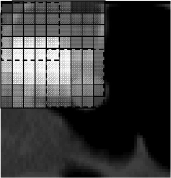
Illustration of highly overlapping training subvolumes. For simplicity, a 5 × 5 2-D subregion is used in this illustration. A subregion overlaps 80% of the next subregion. The subregion at the top left corner (enclosed by dashed lines) overlaps 4% of the subregion four pixels to the right and four pixels down from the top left corner one (enclosed by dashed lines).

Another drawback of the original MTANN is that the training is very time-consuming. This is caused by the high dimensionality of the input vector to the linear-output ANN and the large number of training subvolumes extracted from the training volumes. The use of a smaller subvolume can reduce the dimensionality of the input layer. However, the input subvolume to an MTANN has to be large enough to cover a sufficient part of a polyp candidate. A practical choice of a sphere-shaped subvolume gives n = 171 (see Fig. 2). This also limits the application of an MTANN to polyp candidates of large size. For reducing the training time, one possibility is to reduce the number of training subvolumes. The reduction of the number of training patterns, however, will obviously lead to an insufficiently trained MTANN and directly make the MTANN lose the power to distinguish polyps from non-polyps. To address the issue of dimensionality, we employed an unsupervised dimensionality reduction technique for reducing the dimensionality of the input layer.

Fig. 2.

Dimensionality reduction of the scanning spherical input subvolume to the linear-output ANN via Laplacian eigenfunctions. Each square matrix represents a cross section at a certain z position in the input subvolume, where z₀ represents the central slice of the subvolume. A gray square in each section indicates the input voxel to the linear-output ANN, and a white square indicates an unused voxel. The 171-dimensional original input vector is converted to the Laplacian eigenfunction (LAP) vector. The top n LAPs are extracted and entered to the linear-output ANN.

Dimensionality reduction techniques have long been an active research topic in pattern recognition and many other fields. The generic formulation of dimensionality reduction is stated as follows: Given a set of points I₁,..., I_N in ${\Re }^n$, find a set of points C₁,..., C_N in ${\Re }^d(d\ll n)$ such that C_i “represents” I_i well. PCA is perhaps one of the most popular linear dimension reduction methods because of its relative simplicity and effectiveness [34]. With the increasing research interests in reproducing kernel Hilbert space, a nonlinear extension of PCA based on kernel methods has been proposed in [35]. Other nonlinear dimension reduction approaches have also been proposed, such as Isomap [22] and locally linear embedding [36]. Recently, Belkin et al. have presented a dimension reduction method based on manifold embedding with Laplacian eigenfunctions [20]. They assumed that the original data resided in a low-dimensional manifold, and they constructed an adjacency map to approximate the geometric structure. Motivated by the above observation, we propose using Laplacian eigenfunctions to embed the underlying geometric patterns in the input sub-volume, without abuse of the notation denoted as $I\in {\Re }^n$, into a lower-dimensional manifold M and then applying ANN to the embedded patterns $C\in {\Re }^n$, where $d\ll n$. The method not only incorporates the correlation among inputs, but also achieves the dimension reduction of inputs. This implementation procedure is stated below.

• Step 1) Normalization of Data. We first normalize the inputs $\{I_i=(I_i^1,\dots ,I_i^n):i=1,\dots N\}$ by subtracting the sample mean μ = (μ¹,... μⁿ), where ${\mu }^j=(1∕N){\sum }_{i=1}^N{I}_i^j$, for j = 1,..., n, and then dividing by the estimated standard deviation $\sqrt{(1∕N){\sum }_{i=1}^N{(I_i^j-{\mu }^j)}^2}$. We will use B to denote the normalized data.

• Step 2) Construction of an adjacency graph. Following the above, we let $r_{ij}={\sum }_{k=1}^n{B}_j^k$ denote the correlation coefficient between B_i and B_j, i, j = 1,..., N. Now let G denote a graph with N nodes. The th node corresponds to the ith input $B_i=(B_i^1,\dots ,B_i^n)$. We connect nodes i to j with an edge if r_ij < ε for some specified constant ε > 0. That is, an edge is put only for close ε-neighbors. This implementation reflects the general phenomenon that faraway nodes are usually less important than close neighbors.

• Step 3) Assigning of a weight matrix. For each connected edge between nodes i and j, we assign the Gaussian weight

  $$W_{ij}=e^{-\frac{{\Vert B_i-B_j\Vert }^2}{i}}$$ (6)

  where t is a suitable constant and t = 1.0 in our computation. Otherwise, we assign W_ij = 0. Thus, W is a symmetric matrix. The weight matrix W approximates the manifold structure of the inputs {I_i: i = 1,..., N} in an intrinsic way. In other words, it models the geometry of inputs by preserving the local structure. The justification for our choice of the Gaussian weight relating to the heat kernel can be found in [20].
• Step 4) Laplacian eigenfunctions and embedding map. Let D be a diagonal matrix whose entries are the row or column sums of W, $D_{ii}={\sum }_j{W}_{ji}$, and let L = D − W be the associated Laplacian matrix. Next, compute the eigenvectors and eigenvalues for the generalized eigendecomposition problem

  $${\mathrm{BLB}}^T\mathbf{v}=\lambda {\mathrm{BDB}}^T\mathbf{v}.$$ (7)

Let V₀,..., Vd−1 be the eigenvectors, ordered according to their eigenvalues, λ₀ < λ₁ < ... < λ_d−1. Let the n × d size transformation matrix be

$${\mathbf{V}}_{\mathrm{lap}}=({\mathbf{v}}_0,{\mathbf{v}}_1,\dots ,{\mathbf{v}}_{d-1}).$$ (8)

The transformed data are given by the linear projection of the original data onto the transformation matrix, i.e., $C_i={\mathbf{V}}_{\mathrm{lap}}^T{B}_i=({\mathbf{f}}_0\left(i\right),\dots ,{\mathbf{f}}_{d-1}\left(i\right))$, where C_i is a d-dimensional vector. The overall embedding map is given as I_i → (f₀(i,..., f_d−1(i)). Laplacian eigenmap embedding is optimal in preserving local information. The generalized eigen-decomposition in (7) is derived from the following optimization problem:

$$\begin{array}{cc}\hfill {\mathbf{v}}_{\mathrm{lap}}=& \underset{{\mathbf{v}}^T{\mathrm{BDB}}^T\mathbf{v}=F}{\arg \min }\sum {\Vert {\mathbf{v}}^T{B}_i-{\mathbf{v}}^T{B}_j\Vert }^2{W}_{ij}\hfill \\ \hfill =& \underset{{\mathbf{v}}^T{\mathrm{BDB}}^T\mathbf{v}=F}{\arg \min }{\mathbf{v}}^T\mathrm{BLB}\mathbf{v}\hfill \end{array}$$ (9)

where F is a constraint to avoid a trivial solution. The optimal manifold embedding aims at minimizing the L₂ distance between transformed data in the low-dimensional manifold weighted by the adjacency matrix. The Laplacian matrix of a graph D is analogous to the Laplace Beltrami operator on manifolds [20].

In the context of dimension reduction, the optimal embedding projection matrix V_lap is trained with all the training data via the generalized eigendecomposition equation, (7). In the testing phase, we apply the projection matrix to each test sample independently and transform it to the low-dimensional space.

D. Simulation Experiments

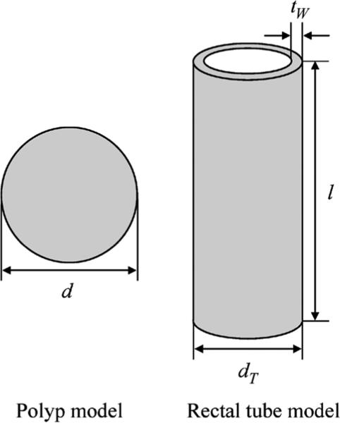
To understand the basic properties of a LAP-MTANN for FP reduction, we carried out an experiment with simulated polyps and rectal tubes, which are one of the major sources of FPs. A polyp is modeled as a sphere with diameter d, and a rectal tube is modeled as a hollow cylinder with diameter d_T, length ln, and wall thickness t_w, as shown in Fig. 4. We employed these simple models with the aim of understanding the essential role of a LAP-MTANN. We trained a LAP-MTANN with ten actual polyps and ten rectal tubes (see the top part of Fig. 3). We did this because this simplified simulated phantom could reveal the fundamental mechanism of the proposed approaches. The simulated CTC volumes with polyps and rectal tubes of five different sizes (d: 6, 8, 10, 12, 15, and 25 mm; d_T: 10, 12, 14, 15, and 16 mm) are illustrated in the top part of Fig. 4.

Fig. 4.

Polyp phantom (a sphere) and a rectal tube phantom (a hollow cylinder). These simple phantom models are employed for understanding the essential role of a LAP-MTANN.

According to the measurements of actual polyps and rectal tubes in clinical CTC volumes, the CT values for the simulated polyps and rectal tubes were set to 60 and 180, respectively. The length ln was 70 mm and the wall thickness t_w was 2 mm.

E. Experiments With Actual CTC Data

To evaluate and compare our proposed 3-D LAP-MTANNs with the original 3-D MTANNs, we carried out experiments with actual polyps and non-polyps in our CTC database.

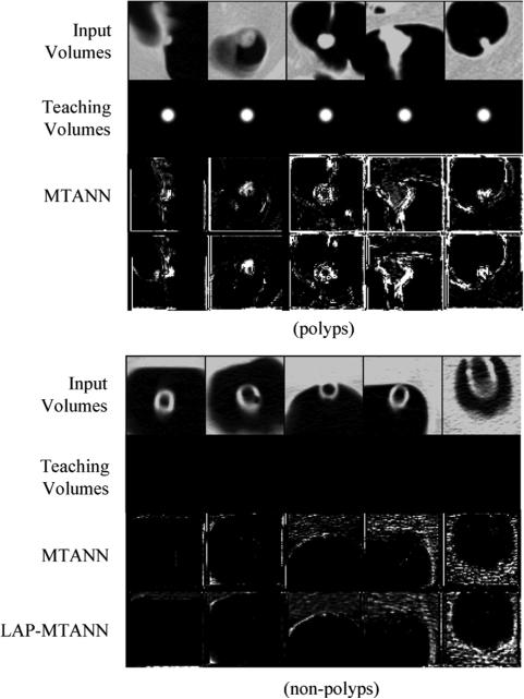
Ten representative polyp volumes (the same actual polyps as used above for simulation) from 46 true-positive volumes in our CTC database and ten non-polyp volumes from the training set were selected manually as the training cases for a 3-D MTANN (see the top part of Fig. 5). The selection was based on the visual appearance of polyps and non-polyps in terms of size, shape, and contrast to represent the database. A three-layer structure was employed for the 3-D MTANN, because it has been shown theoretically that any continuous mapping can be approximated by a three-layer ANN. Based on our previous studies [1], [2], the size of the training volume and the standard deviation of the 3-D Gaussian distribution were selected to be 15 × 15 × 15 voxels and 4.5 voxels, respectively. A quasisphere cubic subvolume of kernel size 7 × 7 × 7 containing 2×(9+21)+3×37 = 171 voxels was employed as the input subvolume for a 3-D MTANN, as shown in Fig. 2 above. Thus, the input layer of the original MTANN has 171 units. The training subvolumes were sampled by every other voxel in each dimension; thus, the total number of training subvolumes for both true positives (TPs) and FPs were 8 × 8 × 8 × 20 = 10240. This sampling scheme also explains the strong dependence structure among the closely sampled patterns which are measured by the correlation coefficient r_ij for the i and jth patterns; see Section II-C for details. The number of hidden units was determined to be 25 by an algorithm for designing the structure of an ANN [37].

Fig. 5.

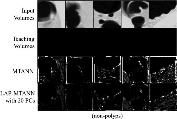
Illustrations of training polyps and the corresponding output volumes of the trained original 3-D MTANN and 3-D LAP-MTANNs with top 20 eigenfunctions and rectal tubes and the corresponding output volumes of the original 3-D MTANN and 3-D LAP-MTANNs in a resubstitution test. Shown are the central axial slices of 3-D volumes. Teaching volumes for polyps contain 3-D Gaussian distributions at the center, whereas those for non-polyps are completely dark, i.e., the voxel values for non-polyps are zero. In the output volumes of the original 3-D MTANN and the 3-D LAP-MTANNs, polyps are represented by bright voxels, whereas non-polyps are dark.

We used receiver-operating-characteristic (ROC) analysis [38] to assess the performance of the original MTANN and the LAP-MTANN in the task of distinguishing polyps from non-polyps. The area under the maximum-likelihood-estimated binormal ROC curve (AUC) was used as an index of performance. We used ROCKIT software [46] to determine the p-value of the difference between two AUC values [39]. For the evaluation of the overall performance of a CAD scheme with 3-D LAP-MTANNs, free-response ROC (FROC) analysis was used [40].

III. Results

A. Simulation Experiments

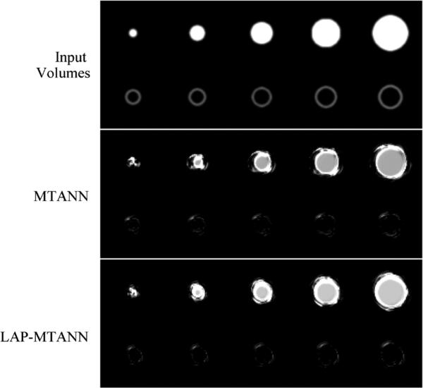
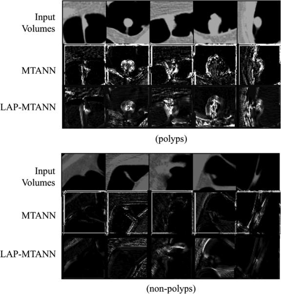
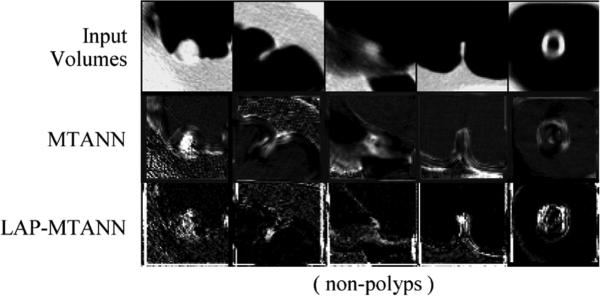
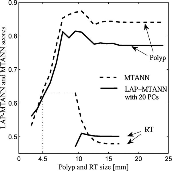
The actual training rectal tubes and their output volumes of the trained 3-D LAP-MTANN with 20 LAPs and the trained original 3-D MTANN were comparable and are illustrated in the lower part of Fig. 5. Both output volumes were well suppressed around the rectal-tube locations. The simulated polyps and rectal tubes and their output are illustrated in Fig. 6. Polyps are represented by bright voxels, whereas rectal tubes appear mostly dark with some bright segments around them. Overall, the LAP-MTANN performed comparably to the MTANN; see Figs. 7 and 8 for the illustration on polyps and non-polyps. The LAP-MTANN performed better than the original MTANN for some polyps and non-polyps, whereas the original MTANN did better for several cases, as seen in Fig. 9 for selected ROIs for illustration. The scores [defined in (4)] of the 3-D LAP-MTANN and the original 3-D MTANN for various-sized simulated polyps and rectal tubes are shown in Fig. 10. The original 3-D MTANN scores for polyps smaller than 4.5 mm overlapped with those of rectal tubes, indicating that simulated polyps larger than 4.5 mm could be distinguished from rectal tubes. On the other hand, although the difference between the 3-D LAP-MTANN scores for polyps larger than 11 mm and for rectal tubes becomes smaller, there was no overlap between the curves for polyps and rectal tubes. This result indicates that the performance of the 3-D LAP-MTANN can be superior to that of the original 3-D MTANN in the distinction of polyps from rectal tubes.

Fig. 6.

Illustrations of simulated polyps and rectal tubes and the corresponding output volumes of the original 3-D MTANN and the LAP-MTANN with 20 eigenfunctions.

Fig. 7.

Illustrations of training non-polyps and the corresponding output volumes. The true polyps used for training are the same as for the simulation. The central axial slices of the 3-D volumes are shown.

Fig. 8.

Illustrations of the performance of the trained 3-D original and LAPMTANNs with the top 20 eigenfunctions on polyps and non-polyps, and the corresponding output volumes. The central axial slices of the 3-D volumes are shown. The performance of the LAP-MTANN is comparable to that of the original MTANN.

Fig. 9.

Illustrations of selected non-polyps, where the LAP-MTANN performs better than the original MTANN on the first three and the original MTANN performs better than the LAP-MTANN on the last two. The central axial slices of the 3-D volumes are shown.

Fig. 10.

Effect of the size of simulated polyps on the distinction between simulated polyps and rectal tubes based on LAP-MTANN and MTANN scores. Based on the scores, polyps larger than 4.5 mm can be distinguished from rectal tubes by the original 3-D MTANN, whereas polyps of all sizes can be distinguished from rectal tubes by the 3-D LAP-MTANN with 20 eigenfunctions.

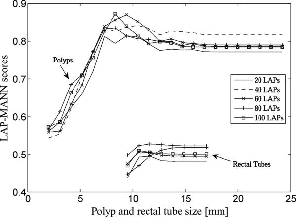
To investigate the effect of different numbers of LAPs used, we plotted the scores of the LAP-MTANNs with various numbers of LAPs for simulated polyps and rectal tubes in Fig. 11. When the number of LAPs increased from 20 to 100, the scores varied slightly, but had the same trend. The maximum scores for rectal tubes were well separated from the minimum scores for polyps. This adds evidence that the classification performance of the LAP-MTANNs with different numbers of LAPs is approximately at the same level. To investigate the effect of different scanning kernel sizes of subvolumes on the performance of a LAP-MTANN, we trained the LAP-MTANN with a larger kernel size of 9 × 9 × 9 voxels (437 voxels in each spherical subvolume). We used the top 20 LAPs for this larger-kernel LAP-MTANN. The training time for this LAP-MTANN was about 4 h, which was the same as that with a kernel size of 7 × 7 × 7 voxels, because the numbers of LAPs and training subvolumes were the same. It turns out that the scores for simulated polyps and rectal tubes dropped almost uniformly from a kernel size of 7 to that of 9, and there is no obvious advantage to employing large kernels in this case.

Fig. 11.

LAP-MTANN scores with various numbers of selected top Laplacian eigenfunctions in the distinction between simulated polyps and rectal tubes.

B. Training

We trained an original 3-D MTANN with the parameters described in the previous section. The training with 500 000 iterations took 38 h, and the mean absolute error between the teaching and output values converged approximately to 0.091. To compare with the proposed LAP-MTANN, we used all of the same above data and parameters with 20 top LAPs (i.e., n = 20). Certainly, different numbers of top LAPs selected would change the result slightly, but the difference was not statistically significant in our studies. We will further justify our choice of n below. The training of a LAP-MTANN was performed with 500 000 iterations, and the mean absolute error converged approximately to 0.10. The training time was reduced substantially to 4 h.

C. Evaluation of the Performance of LAP-MTANNs

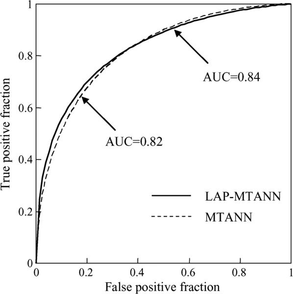
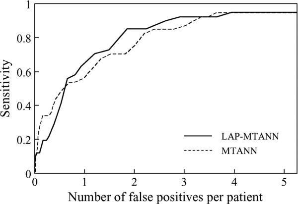
Table I shows the effect of various numbers of top LAPs on the performance of LAP-MTANNs in the distinction between actual polyps and non-polyps. The AUC values of the 3-D LAP-MTANNs with various numbers of LAPs were statistically significantly different from that of the original 3-D MTANN. The ROC curve of the 3-D LAP-MTANN with 20 LAPs is plotted in Fig. 12 together with that of the original MTANN. Fig. 13 shows FROC curves indicating the overall performance of the original 3-D MTANN and the 3-D LAP-MTANN for FP reduction. The original MTANN was able to eliminate 31% (151/489) of FPs without removal of any of the 18 TPs, i.e., a 95% (18/19) overall by-polyp sensitivity was achieved with 3.6 (338/93) FPs per patient. The LAP-MTANN achieved a comparable performance: it eliminated 25% (122/489) of FPs without removal of any TPs. At a sensitivity of 89% (17/19), the original MTANN produced 3.3 (308/92) FPs per patient, whereas the LAP_MTANN produced 2.9 (271/489) FPs per patient.

TABLE I.

Comparisons of the Performance (AUC Values) of LAP-MTANNs With Various Numbers of Top LAPs in the Distinction Between Actual Polyps and Non-Polyps. AUC Values,Standard Errors (SE) of AUC Values, and the P Values for the AUC Difference Between Each LAP-MTANN and the Original MTANN are Shown

MTANN						LAP-MTANN
# of LAPs	-	10	20	30	40	50	60	70	80	90	100	110
AUC	0.82	0.81	0.84	0.83	0.81	0.83	0.84	0.84	0.83	0.83	0.86	0.85
SE	0.03	0.03	0.03	0.03	0.03	0.03	0.03	0.03	0.03	0.03	0.03	0.03
p value	-	0.06	0.48	0.16	0.06	0.46	0.32	0.26	0.35	0.47	0.25	0.30

Fig. 12.

Comparison between the performance of the LAP-MTANN with 20 Laplacian eigenfunctions and that of the original MTANN. The difference between the AUC values for the ROC curves was not statistically significant (p = 0.48).

Fig. 13.

FROC curves indicating the performance of the LAP-MTANN with 20 Laplacian eigenfunctions and that of the original MTANN.

D. Analysis of the Performance of Laplacian Eigenmaps for Dimension Reduction

In order to gain further insights into Laplacian eigenmaps, we investigated the performance of Laplacian eigenmaps for dimension reduction from the pattern recognition perspective. To evaluate the fit of Laplacian eigenmaps, we used the residual variance defined as

$$1-R^2(\widehat{L},L)$$ (10)

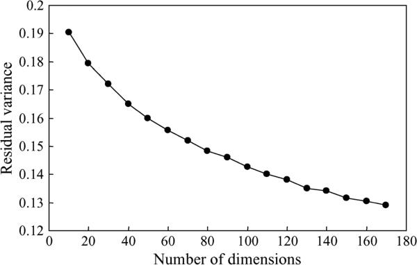
where L is the Laplacian matrix of the original data in the high-dimensional space, L̂ is the matrix of the Euclidean distance in the low-dimensional embedding recovered by the algorithm, R and is the correlation coefficient over all entries of two matrices. The residual variance measures how well the low-dimensional embedding represents the original data in the high-dimensional space. Fig. 14 plots the residual variance as a function of different numbers of dimensions after applying Laplacian eigen-maps to the entire training data. The residual variance decreases as the dimensionality d increases. The curve does not show an “elbow” at which the curve ceases to decrease significantly with extra dimensionalities, which is an indication of intrinsic dimensionality. This is usually the case for real-world data.

Fig. 14.

Residual variances with different numbers of dimensions after application of Laplacian eigenmaps to the entire training data for dimension reduction.

IV. Discussion

In the scheme of MTANN, the input patterns consist of a large number (171 in this study) of neighboring voxel values. Many of these voxels are redundant and may contain much noise in the dataset. On the one hand, large volumes of patterns require a long time for training; on the other hand, this can make the classification task more difficult because of the curse of dimensionality. A reduction of the training time is necessary for practical clinical applications. Dimension reduction can reduce the training time considerably and improve the performance of an MTANN significantly. In our proposed procedure, we first apply the classical PCA to eliminate noise in the data. The PCs of input voxels are the linear combinations of voxels which preserve the variations in the data. The variations of the PCs of the voxel values can approximate the variations of the underlying features. However, the patterns actually overlap close-by patterns. The more they overlap, the more they depend on each other. These close patterns usually have some intrinsic manifold structures, and this information can be employed for more accurately embedding the patterns in a lower-dimensional space.

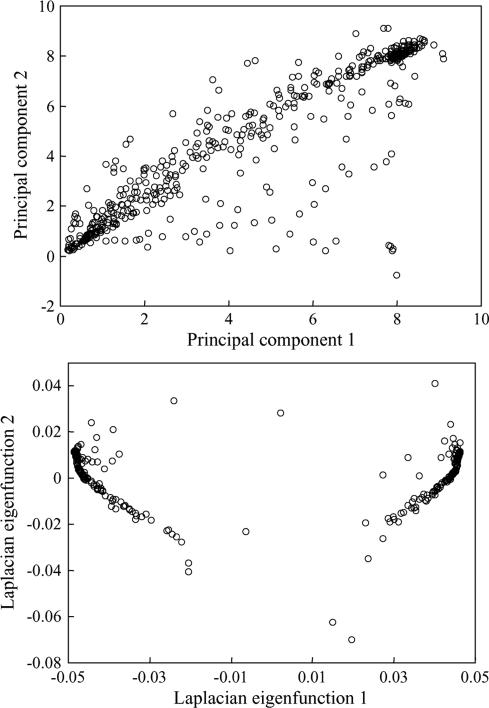
Laplacian eigenfunctions are a well-known manifold learning technique for dimension reduction. They construct a graph by regarding each pattern as a node and then compute the graph Laplacian eigenfunctions. In our proposed scheme, we measure the dependence of patterns by correlation coefficients and map the close-by patterns to close-by points in the reduced lower dimensional space via the Laplacian eigenfunctions. Fig. 15 is an illustration of a subset of 512 training patterns selected from a polyp. One can observe that the top Laplacian functions can learn the intrinsic dependence structures and map close ones to their clusters, whereas the classical PCs just spread the patterns out. Thus, the Laplacian approach fits the MTANN scheme very well. We note that other closely related manifold-based dimension reduction techniques have also been employed in CAD, for example by Summers et al. [41], who have applied a diffusion map for feature selection purposes, which is different from our usage.

Fig. 15.

The top two PCs (upper graph) and Laplacian eigenfunctions (lower graph) of a set of 512 training patterns.

Various manifold learning techniques for dimension reduction have been proposed. The kernel PCA [42] is one of the most widely used methods for dimension reduction. The kernel PCA projects original data into a high-dimensional feature space via a positive definite kernel function and performs PCA in that space. The kernel PCA has been applied successfully to denoising [42] and other areas [43]. On the other hand, Laplacian eigenmaps deal with data in the original input space, and the generalized eigendecomposition is applied to the adjacency graph weight matrix directly. Thus, these two methods are two different techniques in nonlinear dimension reduction. Kernel PCA aims at preserving global properties, whereas Laplacian eigenmaps try to capture neighborhood information of the data. In our application, the neighborhood dependency information is essentially important, because this is how subvolumes are extracted (please see Section II-B for details). Therefore, Laplacian eigenmaps would be more suitable in this particular application.

In practice, one trains each specific LAP-MTANN for each specific type of FPs beforehand and then applies trained LAPMTANNs to process CTC cases. Note that the processing time of new CTC cases has also been reduced to about one tenth of the original MTANN processing time of about 11.7 s per patient based on our database. Nevertheless, the CTC diagnosis is not necessarily real-time. The accuracy in terms of AUC values has also improved slightly from 0.82 to 0.84. We expect that further greater improvement can be obtained in practice, because multiple LAP-MTANNs would be applied, with each trained for a specific task.

The training of an original 3-D MTANN took 38 h. By incorporating Laplacian-eigenfunction-based dimension reduction, we reduced the training time substantially to 4 h. Once trained, the processing time of an original 3-D MTANN and that of a LAP-MTANN are both short, i.e., 11.7 s and 1.16 s per patient, respectively. In the development stage of a new CAD scheme, however, one may want to change the parameters of an MTANN, training cases for the MTANN, and the parameters of an initial detection scheme to optimize the entire CAD scheme. In this case, MTANNs need to be trained a number of times. One can see the result of a LAP-MTANN after 4 h, whereas the result of an original MTANN can be seen after 38 h. Moreover, when a mixture of expert MTANNs is used for reducing a large variety of FPs, the training time increases as the number of MTANNs increases. If six MTANNs are used, the training of an original mixture of expert MTANNs and that of a mixture of expert LAP-MTANNs take 244 (more than 10 days) and 24 h, respectively. Therefore, a LAP-MTANN is desirable especially in the development stage.

One limitation of the study is the use of a limited number of cases with polyps in our study. Evaluation with use of a larger database will generally give more reliable results regarding the performance of a LAP-MTANN. However, it should be noted that, although the 3-D LAP-MTANN trained with only 10 polyps, the performance for 29 polyps, including the 10 polyps and 19 nontraining polyps, was very similar at a high sensitivity level. This observation indicates the robustness of the 3-D LAP-MTANN and is consistent with the observations in our previous studies [1], [2], [16]–[19], [31], [44], [45]. Thus, we expect that the performance of the 3-D LAP-MTANN on a larger database would be potentially comparable to that demonstrated in this study.

V. Conclusion

We have developed 3-D LAP-MTANNs with the aim of improving the efficiency of an MTANN. With Laplacian eigen-functions, we were able to reduce the time required for training of MTANNs substantially while the classification performance was maintained in terms of the reduction of FPs in a CAD scheme for detection of polyps in CTC.

REFERENCES

- 1.Suzuki K, Yoshida H, Nappi J, Dachman AH. Massive-training artificial neural network (MTANN) for reduction of false positives in computer-aided detection of polyps: Suppression of rectal tubes. Med. Phys. 2006;33(10):3814–3824. doi: 10.1118/1.2349839. [DOI] [PubMed] [Google Scholar]
- 2.Suzuki K, Yoshida H, Nappi J, Armato SG, 3rd, Dachman AH. Mixture of expert 3-D massive-training ANNs for reduction of multiple types of false positives in CAD for detection of polyps in CT colonography. Med. Phys. 2008;35(2):694–703. doi: 10.1118/1.2829870. [DOI] [PubMed] [Google Scholar]
- 3.Summers RM, Beaulieu CF, Pusanik LM, Malley JD, Jeffrey RB, Jr., et al. Automated polyp detector for CT colonography: Feasibility study. Radiology. 2000;216(1):284–290. doi: 10.1148/radiology.216.1.r00jl43284. [DOI] [PubMed] [Google Scholar]
- 4.Summers RM, Johnson CD, Pusanik LM, Malley JD, Youssef AM, et al. Automated polyp detection at CT colonography: Feasibility assessment in a human population. Radiology. 2001;219(1):51–59. doi: 10.1148/radiology.219.1.r01ap0751. [DOI] [PubMed] [Google Scholar]
- 5.Yoshida H, Nappi J. Three-dimensional computer-aided diagnosis scheme for detection of colonic polyps. IEEE Trans. Med. Imag. 2001 Dec;20(12):1261–1274. doi: 10.1109/42.974921. [DOI] [PubMed] [Google Scholar]
- 6.Nappi J, Yoshida H. Feature-guided analysis for reduction of false positives in CAD of polyps for computed tomographic colonography. Med. Phys. 2003;30(7):1592–1601. doi: 10.1118/1.1576393. [DOI] [PubMed] [Google Scholar]
- 7.Paik DS, Beaulieu CF, Rubin GD, Acar B, Jeffrey RB, Jr., et al. Surface normal overlap: A computer-aided detection algorithm with application to colonic polyps and lung nodules in helical CT. IEEE Trans. Med. Imag. 2004 Jun;23(6):661–675. doi: 10.1109/tmi.2004.826362. [DOI] [PubMed] [Google Scholar]
- 8.Kiss G, Van Cleynenbreugel J, Thomeer M, Suetens P, Marchal G. Computer-aided diagnosis in virtual colonography via combination of surface normal and sphere fitting methods. Eur. Radiol. 2002;12(1):77–81. doi: 10.1007/s003300101040. [DOI] [PubMed] [Google Scholar]
- 9.Gokturk SB, Tomasi C, Acar B, Beaulieu CF, Paik DS, et al. A statistical 3-D pattern processing method for computer-aided detection of polyps in CT colonography. IEEE Trans. Med. Imag. 2001 Dec;20(12):1251–1260. doi: 10.1109/42.974920. [DOI] [PubMed] [Google Scholar]
- 10.Acar B, Beaulieu CF, Gokturk SB, Tomasi C, Paik DS, et al. Edge displacement field-based classification for improved detection of polyps in CT colonography. IEEE Trans. Med. Imag. 2002 Dec;21(12):1461–1467. doi: 10.1109/TMI.2002.806405. [DOI] [PubMed] [Google Scholar]
- 11.Jerebko AK, Malley JD, Franaszek M, Summers RM. Multiple neural network classification scheme for detection of colonic polyps in CT colonography data sets. Acad. Radiol. 2003;10(2):154–160. doi: 10.1016/s1076-6332(03)80039-9. [DOI] [PubMed] [Google Scholar]
- 12.Jerebko AK, Summers RM, Malley JD, Franaszek M, Johnson CD. Computer-assisted detection of colonic polyps with CT colonography using neural networks and binary classification trees. Med. Phys. 2003;30(1):52–60. doi: 10.1118/1.1528178. [DOI] [PubMed] [Google Scholar]
- 13.Yao J, Miller M, Franaszek M, Summers RM. Colonic polyp segmentation in CT colonography-based on fuzzy clustering and deformable models. IEEE Trans. Med. Imag. 2004 Nov;23(11):1344–1352. doi: 10.1109/TMI.2004.826941. [DOI] [PubMed] [Google Scholar]
- 14.Iordanescu G, Summers RM. Reduction of false positives on the rectal tube in computer-aided detection for CT colonography. Med. Phys. 2004;31(10):2855–2862. doi: 10.1118/1.1790131. [DOI] [PubMed] [Google Scholar]
- 15.Suzuki K, Armato SG, 3rd, Li F, Sone S, Doi K. Massive training artificial neural network (MTANN) for reduction of false positives in computerized detection of lung nodules in low-dose computed tomography. Med. Phys. 2003;30(7):1602–1617. doi: 10.1118/1.1580485. [DOI] [PubMed] [Google Scholar]
- 16.Suzuki K, Abe H, MacMahon H, Doi K. Image-processing technique for suppressing ribs in chest radiographs by means of massive training artificial neural network (MTANN) IEEE Trans. Med. Imag. 2006 Apr;25(4):406–416. doi: 10.1109/TMI.2006.871549. [DOI] [PubMed] [Google Scholar]
- 17.Suzuki K, Shiraishi J, Abe H, MacMahon H, Doi K. False-positive reduction in computer-aided diagnostic scheme for detecting nodules in chest radiographs by means of massive training artificial neural network. Acad. Radiol. 2005;12(2):191–201. doi: 10.1016/j.acra.2004.11.017. [DOI] [PubMed] [Google Scholar]
- 18.Arimura H, Katsuragawa S, Suzuki K, Li F, Shiraishi J, et al. Computerized scheme for automated detection of lung nodules in low-dose computed tomography images for lung cancer screening. Acad. Radiol. 2004;11(6):617–629. doi: 10.1016/j.acra.2004.02.009. [DOI] [PubMed] [Google Scholar]
- 19.Suzuki K. A supervised ‘lesion-enhancement’ filter by use of a massive-training artificial neural network (MTANN) in computer-aided diagnosis (CAD) Phys. Med. Biol. 2009;54(18):S31–S45. doi: 10.1088/0031-9155/54/18/S03. [DOI] [PMC free article] [PubMed] [Google Scholar]
- 20.Belkin M, Niyogi P. Laplacian Eigenmaps for dimensionality reduction and data representation. Neural Computat. 2003;15(6):1373–1396. [Google Scholar]
- 21.Coifman RR, Lafon S, Lee AB, Maggioni M, Nadler B, et al. Geometric diffusions as a tool for harmonic analysis and structure definition of data: Diffusion maps. Proc. Nat. Acad. Sci. USA. 2005;102(21):7426–7431. doi: 10.1073/pnas.0500334102. [DOI] [PMC free article] [PubMed] [Google Scholar]
- 22.Tenenbaum JB, de Silva V, Langford JC. A global geometric framework for nonlinear dimensionality reduction. Science. 2000;290(5500):2319–2323. doi: 10.1126/science.290.5500.2319. [DOI] [PubMed] [Google Scholar]
- 23.Nappi J, Dachman AH, MacEneaney P, Yoshida H. Automated knowledge-guided segmentation of colonic walls for computerized detection of polyps in CT colonography. J. Comput. Assist. Tomogr. 2002;26(4):493–504. doi: 10.1097/00004728-200207000-00003. [DOI] [PubMed] [Google Scholar]
- 24.He L, Chao Y, Suzuki K, Wu K. Fast connected-component labeling. Pattern Recognit. 2009;42:1977–1987. [Google Scholar]
- 25.He L, Chao Y, Suzuki K. A run-based two-scan labeling algorithm. IEEE Trans Image Process. 2008 May;17(5):749–756. doi: 10.1109/TIP.2008.919369. [DOI] [PubMed] [Google Scholar]
- 26.Suzuki K, Horiba I, Sugie N. Linear-time connected-component labeling based on sequential local operations. Comput. Vis. Image Understand. 2003;89(1):1–23. [Google Scholar]
- 27.Nappi J, Yoshida H. Automated detection of polyps with CT colonography: Evaluation of volumetric features for reduction of false-positive findings. Acad. Radiol. 2002;9(4):386–397. doi: 10.1016/s1076-6332(03)80184-8. [DOI] [PubMed] [Google Scholar]
- 28.Yoshida H, Dachman AH. CAD techniques, challenges, and controversies in computed tomographic colonography. Abdominal Imag. 2005;30(1):26–41. doi: 10.1007/s00261-004-0244-x. [DOI] [PubMed] [Google Scholar]
- 29.Fukunaga K. Introduction to Statistical Pattern Recognition. 2nd ed. Academic; San Diego, CA: 1990. [Google Scholar]
- 30.Suzuki K, Horiba I, Sugie N. Efficient approximation of neural filters for removing quantum noise from images. IEEE Trans. Signal Process. 2002 Jul;50(7):1787–1799. [Google Scholar]
- 31.Suzuki K, Horiba I, Sugie N. Neural edge enhancer for supervised edge enhancement from noisy images. IEEE Trans. Pattern Anal. Mach. Intell. 2003 Dec;25(12):1582–1596. [Google Scholar]
- 32.Suzuki K, Horiba I, Sugie N, Nanki M. Extraction of left ventricular contours from left ventriculograms by means of a neural edge detector. IEEE Trans. Med. Imag. 2004 Mar;23(3):330–339. doi: 10.1109/TMI.2004.824238. [DOI] [PubMed] [Google Scholar]
- 33.Rumelhart DE, Hinton GE, Williams RJ. Learning representations by back-propagating errors. Nature. 1986;323:533–536. [Google Scholar]
- 34.Jolliffe IT. Principal Component Analysis. 2nd ed. Springer; New York: 2002. [Google Scholar]
- 35.Scholkopf B, Smola A, Muller K-R. Nonlinear component analysis as a kernel Eigenvalue problem. Neural Computat. 1998;10:1299–1319. [Google Scholar]
- 36.Roweis ST, Saul LK. Nonlinear dimensionality reduction by locally linear embedding. Science. 2000;290(22):2323–2326. doi: 10.1126/science.290.5500.2323. [DOI] [PubMed] [Google Scholar]
- 37.Suzuki K. Determining the receptive field of a neural filter. J. Neural Eng. 2004;1(4):228–237. doi: 10.1088/1741-2560/1/4/006. [DOI] [PubMed] [Google Scholar]
- 38.Metz CE. ROC methodology in radiologic imaging. Invest. Radiol. 1986;21(9):720–733. doi: 10.1097/00004424-198609000-00009. [DOI] [PubMed] [Google Scholar]
- 39.Metz CE, Herman BA, Shen JH. Maximum likelihood estimation of receiver operating characteristic (ROC) curves from continuously-distributed data. Stat. Med. 1998;17(9):1033–1053. doi: 10.1002/(sici)1097-0258(19980515)17:9<1033::aid-sim784>3.0.co;2-z. [DOI] [PubMed] [Google Scholar]
- 40.Egan JP, Greenberg GZ, Schulman AI. Operating characteristics, signal detectability, and the method of free response. J. Acoust. Soc. Am. 1961;33:993–1007. [Google Scholar]
- 41.Wang S, Yao J, Summers RM. Improved classifier for computer-aided polyp detection in CT colonography by nonlinear dimensionality reduction. Med. Phys. 2008;35(4):1377–1386. doi: 10.1118/1.2870218. [DOI] [PMC free article] [PubMed] [Google Scholar]
- 42.Mika S, Schölkopf B, Müller ASK-R, Scholz M, Rätsch G. Kernel PCA and de-noising in feature spaces. Adv. Neural Inf. Process. Syst. 1999:536–542. [Google Scholar]
- 43.Hoffmann H. Kernel PCA for novelty detection. Pattern Recognit. 2007;40(3):863–874. [Google Scholar]
- 44.Suzuki K, Doi K. How can a massive training artificial neural network (MTANN) be trained with a small number of cases in the distinction between nodules and vessels in thoracic CT? Acad. Radiol. 2005;12(10):1333–1341. doi: 10.1016/j.acra.2005.06.017. [DOI] [PubMed] [Google Scholar]
- 45.Suzuki K, Rockey DC, Dachman AH. CT colonography: Computer-aided detection of false-negative polyps in a multicenter clinical trial. Med. Phys. 2010;30:2–21. doi: 10.1118/1.3263615. [DOI] [PMC free article] [PubMed] [Google Scholar]
- 46.ROCKIT software. ver. 1.1b [Online] Available: http://xray.bsd.uchicago.edu/krl/roc_soft6.htm.