

Abstract
Propensity-score matching is increasingly being used to reduce the confounding that can occur in observational studies examining the effects of treatments or interventions on outcomes. We used Monte Carlo simulations to examine the following algorithms for forming matched pairs of treated and untreated subjects: optimal matching, greedy nearest neighbor matching without replacement, and greedy nearest neighbor matching without replacement within specified caliper widths. For each of the latter two algorithms, we examined four different sub-algorithms defined by the order in which treated subjects were selected for matching to an untreated subject: lowest to highest propensity score, highest to lowest propensity score, best match first, and random order. We also examined matching with replacement. We found that (i) nearest neighbor matching induced the same balance in baseline covariates as did optimal matching; (ii) when at least some of the covariates were continuous, caliper matching tended to induce balance on baseline covariates that was at least as good as the other algorithms; (iii) caliper matching tended to result in estimates of treatment effect with less bias compared with optimal and nearest neighbor matching; (iv) optimal and nearest neighbor matching resulted in estimates of treatment effect with negligibly less variability than did caliper matching; (v) caliper matching had amongst the best performance when assessed using mean squared error; (vi) the order in which treated subjects were selected for matching had at most a modest effect on estimation; and (vii) matching with replacement did not have superior performance compared with caliper matching without replacement. © 2013 The Authors. Statistics in Medicine published by John Wiley & Sons, Ltd.
Keywords: propensity score, matching, computer algorithms, optimal matching, Monte Carlo simulations, propensity-score matching
1 Introduction
There is an increasing interest in estimating the causal effects of treatment using observational or non-randomized data. In observational studies, the baseline characteristics of treated or exposed subjects often differ systematically from those of untreated or unexposed subjects. Essential to the production of high-quality evidence to inform decision-making is the ability to minimize the effect of confounding. An increasingly frequent approach to minimizing bias when estimating causal treatment effects is based on the propensity score 1. The propensity score is the probability of treatment assignment conditional on observed baseline covariates. There are four methods in which the propensity score can be used: matching on the propensity score, stratification on the propensity score, covariate adjustment using the propensity score, and inverse probability of treatment weighting using the propensity score 1,2.
Propensity-score matching is frequently used in the medical and social sciences literatures 3–6. Propensity-score matching involves forming matched sets of treated and untreated subjects that share a similar value of the propensity score. The most common implementation is 1:1 or pair-matching in which pairs of treated and untreated subjects are formed. The effect of treatment on outcomes can be estimated by comparing outcomes between treatment groups in the matched sample. Pair-matching on the propensity score allows one to estimate the average treatment effect in the treated (ATT) 7. In the methodological literature, a wide range of different methods have been proposed for forming matched pairs. These include optimal matching, nearest neighbor matching, and nearest neighbor matching within specified propensity score calipers 8,9. In the medical literature, the latter appears to be the most common matching method, although there is no consistency in the caliper width that is used 3,4. Furthermore, one can consider matching with or without replacement. Matching with replacement and optimal matching appear to be used infrequently in the applied literature. Although prior studies have compared the relative performance of different caliper widths when using nearest neighbor matching within specified caliper widths 10,11, there is a paucity of research comparing different matching algorithms.
The objective of the current paper is to compare the performance of different algorithms for matching on the propensity score. The paper is structured as follows: in Section 2, we describe different matching algorithms. In Section 3, we describe a series of Monte Carlo simulations to examine the performance of these algorithms for estimating linear treatment effects. In particular, we report on bias, variance, mean squared error (MSE), and balance on baseline covariates induced by matching on the propensity score. In Section 4, we present a case study in which we compare the performance of different matching algorithms when estimating the effect of drug prescribing on mortality in a cohort of patients discharged from hospital with a diagnosis of acute myocardial infarction (AMI). Finally, in Section 5, we summarize our findings and place them in the context of the existing literature.
2 Descriptions of algorithms for pair-matching on the propensity score
In this section, we briefly review different algorithms for forming pairs of treated and untreated subjects matched on the propensity score. We describe optimal matching, greedy nearest neighbor matching without replacement, greedy nearest neighbor matching without replacement within specified caliper widths, nearest neighbor matching with replacement, and nearest neighbor matching with replacement within specified caliper widths. We restrict our attention to methods for forming pairs of treated and untreated subjects and do not consider different variations of many-to-one matching.
We first consider methods based on matching without replacement. Using this approach, we matched each untreated subject to at most one treated subject. Once an untreated subject has been matched to a treated subject, that untreated subject is no longer eligible for consideration as a match for other treated subjects. The primary distinction between different matching algorithms that use matching without replacement is between optimal matching and methods based on greedy matching 8. Optimal matching forms matched pairs so as to minimize the average within-pair difference in propensity scores. In contrast, greedy nearest neighbor matching selects a treated subject and then selects as a matched control subject, the untreated subject whose propensity score is closest to that of the treated subject (if multiple untreated subjects are equally close to the treated subject, one of these untreated subjects is selected at random). We examined four different approaches to greedy nearest neighbor matching. First, we selected sequentially treated subjects from highest to lowest propensity score; second, we selected sequentially treated subjects from lowest to highest propensity score; third, we selected sequentially treated subjects in the order of the best possible match. Thus, the first selected treated subject was that treated subject who was closest to an untreated subject. The second selected treated subject was that treated subject who was closest to the remaining untreated subjects; fourth, we selected treated subjects in a random order. When using this last approach, one can use a fixed random number seed so that the matched sample is reproducible in subsequent analyses. We refer to these four algorithms as greedy nearest neighbor matching (high to low), greedy nearest neighbor matching (low to high), greedy nearest neighbor matching (closest distance), and greedy nearest neighbor matching (random), respectively.
A modification to greedy nearest neighbor matching is greedy nearest neighbor matching within specified caliper widths. In this modification to greedy nearest neighbor matching, we can match treated and untreated subjects only if the absolute difference in their propensity scores is within a prespecified maximal distance (the caliper distance). When using caliper matching, we matched subjects on the logit of the propensity score using a caliper width that was defined as a proportion of the standard deviation of the logit of the propensity score 9,12. Although it may appear inconsistent to have some methods be based on matching on the propensity score whereas other methods are based on matching on the logit of the propensity score, there are valid reasons for this discrepancy. Matching on the propensity score would appear to be the natural metric to use, and we have used it as the default approach. However, when using caliper matching, we have chosen to match on the logit of the propensity score because the reduction in bias due to the use of different caliper widths has been described when matching on the logit of the propensity score 9. Because there are theoretical justifications for the choice of different calipers when matching on the logit of the propensity score, we have elected to use this approach for the caliper-based matching algorithms. We examined greedy nearest neighbor matching (high to low) within specified caliper widths, greedy nearest neighbor matching (low to high) within specified caliper widths, greedy nearest neighbor matching (closest distance) within specified caliper widths, and greedy nearest neighbor matching (random order) within specified caliper widths.
Optimal matching and greedy nearest neighbor matching on the propensity score will result in all treated subjects being matched to an untreated subject (assuming that the number of untreated subjects is at least as large as the number of treated subjects). However, greedy nearest neighbor matching within specified caliper widths may not result in all treated subjects being matched to an untreated subject, because for some treated subjects, there may not be any untreated subjects who are unmatched and whose propensity score lies within the specified caliper distance of that of the treated subject.
All of the methods described earlier used matching without replacement: once an untreated subject had been matched to a given treated subject, that untreated subject is no longer eligible for consideration as a match for a subsequent treated subject. Thus, we could include each untreated subject in at most one matched pair in the final matched sample. The final two algorithms that we considered used matching with replacement. Matching with replacement permits the same untreated subject to be matched to multiple treated subjects. We considered nearest neighbor matching with replacement and nearest neighbor matching within specified caliper widths with replacement. Each of these approaches simply matches each treated subject to the nearest untreated subject (subject to possible caliper restrictions). Because untreated subjects are recycled or allowed to be included in multiple matched sets, the order in which the treated subjects are selected has no effect on the formation of matched pairs.
3 Monte Carlo simulations
We used a series of Monte Carlo simulations to compare the performance of different algorithms for matching on the propensity score. We assessed the performance of each algorithm using the following four criteria: (i) bias in estimating linear treatment effects; (ii) variance of the estimated treatment effect; (iii) the MSE of estimated linear treatment effects; and (iv) the ability to induce balance on measured baseline covariates.
3.1 Monte Carlo simulations–methods
We based the design of our Monte Carlo simulations on a prior study that examined the performance of different caliper widths for use with greedy nearest neighbor caliper matching 11. As in the prior study, we assumed that there were 10 covariates (X1 − X10) that effected either treatment selection or the outcome. The treatment-selection model was logit(pi,treat) = α0,treat + αLx1,i + αLx2,i + αMx4,i + αMx5,i + αHx7,i + αHx8,i + αVHx10,i. For each subject, we generated treatment status (denoted by z) from a Bernoulli distribution with parameter pi,treat. For each subject, we generated both a continuous and a dichotomous outcomes. We generated the continuous outcome using the following model: yi = β0 + zi + αLx2,i + αLx3,i + αMx5,i + αMx6,i + αHx8,i + αHx9,i + αVHx10,i + ɛi, where ɛi ∼ N(0,σ = 3). Thus, treatment increased the mean response by one unit (thus, the ATT was 1). For each subject, we also generated a dichotomous outcome using the following logistic model: logit(pi,outcome) = β0,outcome + βtreatzi + αLx2,i + αLx3,i + αMx5,i + αMx6,i + αHx8,i + αHx9,i + αVHx10,i. We then generated a binary outcome for each subject from a Bernoulli distribution with parameter pi,outcome. We selected the intercept, β0,outcome, in the logistic outcome model so that the incidence of the outcome would be approximately 0.10 if all subjects in the population were untreated. This is approximately equal to the proportion of patients hospitalized with an AMI who are readmitted within 1 year (11%) and to the 30-day mortality rate for hospitalized AMI patients (12%) 13,14. In a given simulated dataset, we simulated a binary outcome for each subject, under the assumption that all subjects were not treated (z = 0). We then calculated the incidence of the outcome in the simulated dataset. We used a bisection approach to determine that value of β0,outcome that would result in an incidence of 0.10. We set the regression coefficients αL, αM, αH, and αVH to log(1.25), log(1.5), log(1.75), and log(2), respectively. Thus, there were two covariates that had a weak effect on each of treatment selection and outcomes, two covariates that had a moderate effect on each of treatment selection and outcomes, two covariates that had a strong effect on each of treatment selection and outcomes, and one covariate that had a very strong effect on both treatment selection and outcomes. We selected the conditional log-odds ratio, βtreat, using methods described elsewhere so that average absolute risk reduction in treated subjects due to treatment would be 0.02 15 (i.e., the true ATT was − 0.02). Briefly, for a given value of βtreat, we determined the probability of the occurrence of the outcome for each subject twice: first, under the assumption that the subject was untreated; second, under the assumption that the subject was treated. The subject-specific risk-difference was the difference between these two probabilities. We then determined the average subject-specific risk-difference across all subjects who ultimately received the treatment (because we are focusing on the ATT). We used an iterative process to determine the value of βtreat that would result in the desired risk difference ( − 0.02). We performed this iterative process prior to the main body of simulations. Thus, we used the same value of βtreat in all 1000 simulated datasets in a given scenario. Because we were simulating data with a desired ATT, the value of βtreat would depend on the proportion of subjects that were treated. Note that this approach allows for variation in subject-specific treatment effects (or differences in risk). We used a logistic model to simulate data with an underlying average treatment effect in the treated because such an approach will guarantee that individual probabilities of the occurrence of the outcome will lie within the unit interval. Although the use of a linear model to generate probabilities would result in a linear treatment effect on the probability scale, such an approach could result in subjects whose probabilities of the occurrence of the outcome lie outside of the unit interval (and thus violate the definition of a probability). The use of an appropriate link function will constrain predicted probabilities to lie within the unit interval, regardless of the values taken by the baseline covariates. The adopted approach results in a uniform effect of treatment on the relative odds scale, whereas the absolute effect of treatment may vary across subjects. However, this may be reflective of many clinical scenarios, because the absolute risk reduction may be greater for subjects at a greater baseline risk of the event compared with subjects with a lower baseline risk of the event. Despite potential non-uniformity of the absolute risk reduction, clinical investigators are still interested in estimating the average risk difference over the population (or over the treated subjects).
Our Monte Carlo simulations had a complete factorial design in which the following two factors were allowed to vary: (i) the distribution of the 10 baseline covariates; and (ii) the proportion of subjects who received the treatment. We considered five different distributions for the 10 baseline covariates: (a) the 10 covariates had independent standard normal distributions; (b) the 10 covariates were from a multivariable normal distribution. Each variable had mean zero and unit variance, and the pair-wise correlation between variables was 0.25; (c) the first five variables were independent Bernoulli random variables each with parameter 0.5, whereas the second five variables were independent standard normal random variables; (d) the 10 random variables were independent Bernoulli random variables, each with parameter 0.5; and (e) the 10 random variables were correlated Bernoulli random variables. In this setting, 10 continuous variables were generated as in scenario (b). Each continuous variable was then dichotomized at the population mean (zero). In a prior study, Austin 11 used the first four of these scenarios (a–d), whereas the fifth scenario was added to the current study. In a clinical context, the continuous variables can represent variables such as demographic characteristics (age, years of education, or income), vital signs (systolic and diastolic blood pressure, heart rate, and respiratory rate), and results of laboratory testing (e.g., hemoglobin, lipid levels, and creatinine). The dichotomous variables can represent demographic characteristics (sex) or the presence or absence of risk factors and co-existing illnesses (e.g., diabetes, hypertension, and kidney disease). For the second factor, we considered five different levels for the proportion of subjects that were treated: 0.05, 0.10, 0.20, 0.25, and 0.33. We modified the value of α0,treat in the treatment-selection model to obtain the desired prevalence of treatment in the simulated datasets. We thus considered 25 different scenarios: five different distributions for the baseline covariates times five levels of the proportion of subjects who were treated (0.05, 0.10, 0.20, 0.25, and 0.33).
In each of the 25 scenarios, we simulated 1000 datasets, each consisting of 1000 subjects. The decision to use simulated datasets of size 1000 was made for two reasons. First, matching algorithms can be computationally intensive. Because 12 different matching algorithms were being examined, the decision was made to use datasets of moderate size. Second, in a systematic review of the use of propensity score methods in the medical literature, we observed that these methods have been used in datasets of size less than 1000 16. In each simulated dataset, we estimated the propensity score using a logistic regression model to regress treatment assignment on the seven variables that affect the outcome. We selected this approach as it has been shown to result in superior performance compared with including all measured covariates or those variables that affect treatment selection 17. In practice, one can use the existing literature and clinical or subject-matter knowledge and expertise to identify those variables that affect the outcome. It is likely that this set of variables will be relatively consistent across regions or jurisdictions, whereas the set of variables that affect treatment selection may vary between regions or jurisdictions. In each simulated dataset, we used 12 different matching algorithms to match treated subjects to untreated subjects: optimal matching (on the propensity score and on the logit of the propensity score), greedy nearest neighbor matching (high to low), greedy nearest neighbor matching (low to high), greedy nearest neighbor matching (closest distance), greedy nearest neighbor matching (random order), caliper matching (low to high), caliper matching (high to low), caliper matching (closest distance), caliper matching (random order), nearest neighbor matching (with replacement), and caliper matching (with replacement). For the nearest neighbor matching algorithms, we matched subjects on the propensity score, whereas in the caliper matching algorithms, we matched subjects on the logit of the propensity score using a caliper of width equal to 0.2 of the standard deviation of logit of the propensity score 11. Thus, in each simulated dataset, we formed 12 matched sets.
In each matched set, we estimated the estimated treatment effect as the difference between the mean of the observed outcome in treated subjects in the matched sample and the mean of the observed outcome in untreated subjects in the matched sample:  , where Y1,i and Y0,i denote the outcome for the ith treated subject and ith untreated subject in the matched sample, respectively (and where the matched sample consists of N matched pairs). Thus, we estimated both a difference in means (continuous outcome) and a risk difference (binary outcome) in the propensity-score matched sample. This estimator removes the effect of confounding because the distribution of baseline covariates is expected to be the same in treated and untreated subjects in the matched sample 1. We also computed the absolute standardized difference comparing the distribution of each of the 10 baseline covariates between treatment groups in each of the matched samples 18,19. For continuous variables, the standardized difference is defined as
  where
where  and
and  denote the sample mean of the covariate in treated and untreated subjects, respectively, whereas
  and
and  denote the sample variance of the covariate in treated and untreated subjects, respectively. For dichotomous variables, the standardized differences are defined as
  , where
  and
and  denote the prevalence or mean of the dichotomous variable in treated and untreated subjects, respectively. For caliper matching, we determined the mean percentage of treated subjects that were matched to an untreated subject (for the other matching algorithms, 100% of treated subjects will be matched to an untreated subject because there is no restriction on the maximum difference in the propensity scores for a matched pair).
Let θ denote the true treatment effect (1 and − 0.02 for continuous and binary outcomes, respectively), and let θi denote the estimated treatment effect in the ith simulated sample (i = 1, … ,1000). We estimated the mean estimated treatment effect as  and the MSE as
  . For each of the 10 baseline covariates, we estimated the mean absolute standardized difference across the 1000 simulated datasets.
3.2 Monte Carlo simulations–results
To provide a context for the estimated treatment effects obtained using different matching algorithms, we examined the mean estimated crude or unadjusted treatment effects across the 25 different scenarios. The minimum and maximum crude treatment effects for the continuous outcome were 1.20 (percent bias: 20%) and 3.46 (percent bias: 246%). The first and third quartiles were 1.53 (53%) and 1.88 (88%), respectively. The minimum and maximum crude treatment effects for the binary outcome were 0 (percent bias: − 100%) and 0.238 (percent bias: − 1292%). The first and third quartiles were 0.026 ( − 232%) and 0.062 ( − 412%), respectively. These summary statistics allow one to examine the degree to which bias was reduced by using different matching algorithms.
The results for optimal matching on the propensity score were the same as those for optimal matching on the logit of the propensity score. In order to simplify the presentation of our results, we do not present results for the latter algorithm. Optimal matching, greedy nearest neighbor matching without replacement, and greedy nearest neighbor matching with replacement result, by design, in 100% of treated subjects being included in the matched sample. For the different caliper matching algorithms, the average percentage of treated subjects matched to an untreated subject in each of the 25 scenarios is described in Figure A1 in the Supporting information. For each of the five sets of distributions for the baseline covariates, the percentage of treated subjects successfully matched to an untreated subject was highest when caliper matching with replacement was used. The rank ordering of the four caliper methods that used matching without replacement was (from highest percentage of matched subjects to lowest percentage) selecting treated subjects from highest to lowest propensity score, selecting treated subjects at random, sequentially selecting treated subjects from best to worst match, and sequentially selecting treated from lowest to highest propensity score. The differences between caliper matching (highest to lowest) without replacement and the three other methods that used matching without replacement tended to increase as the prevalence of treatment increased (i.e., differences between caliper matching (highest to lowest) without replacement and the three other methods were the smallest when 5% of subjects were treated, whereas it was the greatest when 33% of subjects were treated).
The mean within-pair difference in the propensity score for the different matching algorithms is reported in Figure A2 in the Supporting information. Greedy nearest neighbor matching (lowest to highest) tended to result in mean differences in the propensity score that were greater than those from all other matching methods. Optimal matching tended to result in performance similar to that of three of the methods based on nearest neighbor matching without replacement (high to low, random, and closest distance). As would be expected, matching without replacement resulted in matched samples with the lowest mean within-pair difference in the propensity score. Caliper matching without replacement tended to have a performance between that of the nearest neighbor matching without replacement algorithms and the methods that used matching with replacement.
We report the mean estimated linear treatment effects in Figure 1 (continuous outcome) and Figure 2 (binary outcome). Recall that the true treatment effects were 1 and − 0.02, respectively. A horizontal line has been added to each panel denoting the magnitude of the true treatment effect. In general, optimal matching and nearest neighbor matching without replacement tended to have similar performance. Bias tended to be less with nearest neighbor caliper matching and matching with replacement. Amongst the methods that used caliper matching without replacement, bias tended to be less when treated subjects were selected in a random order or sequentially in the order of best match first.
Figure 1.
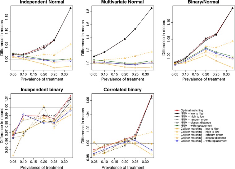
Treatment effect: difference in means.
Figure 2.
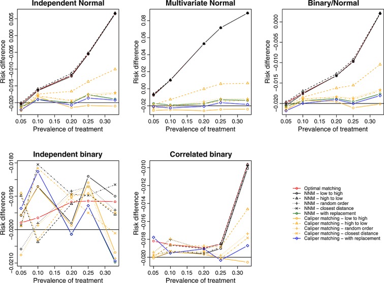
Treatment effect: risk difference.
We report the standard deviations of the estimated treatment effects across the 1000 simulated datasets for each scenario in Figure 3 (continuous outcome) and Figure A3 in the Supporting information (binary outcome). Matching with replacement tended to result in estimates that displayed greater variability than the methods based on matching without replacement. When at least some of the covariates were normally distributed and the outcome was continuous, optimal matching and the four implementations of nearest neighbor matching without replacement tended to result in estimates that displayed slightly less variability than the methods based on caliper matching without replacement.
Figure 3.
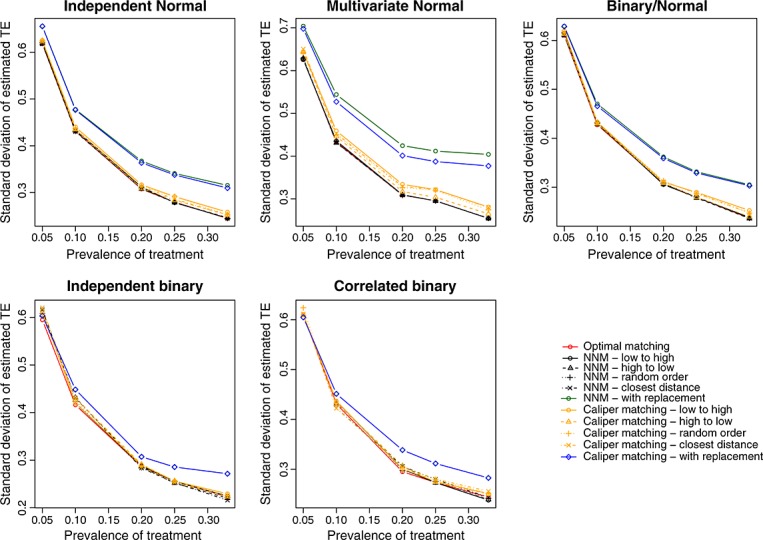
Standard deviation of estimated difference in means.
We report the MSE of the estimated treatment effects in Figure 4 (continuous outcome) and Figure 5 (binary outcome). Matching with replacement tended to result in estimates with greater MSE compared with methods based on matching without replacement. The four different nearest neighbor caliper matching algorithms that used matching without replacement tended to have very similar performance to one another. In some settings, they had very similar performance to optimal matching and to nearest neighbor matching without replacement. However, in a minority of scenarios, their performance substantially exceeded that of optimal matching and that of nearest neighbor matching without replacement.
Figure 4.
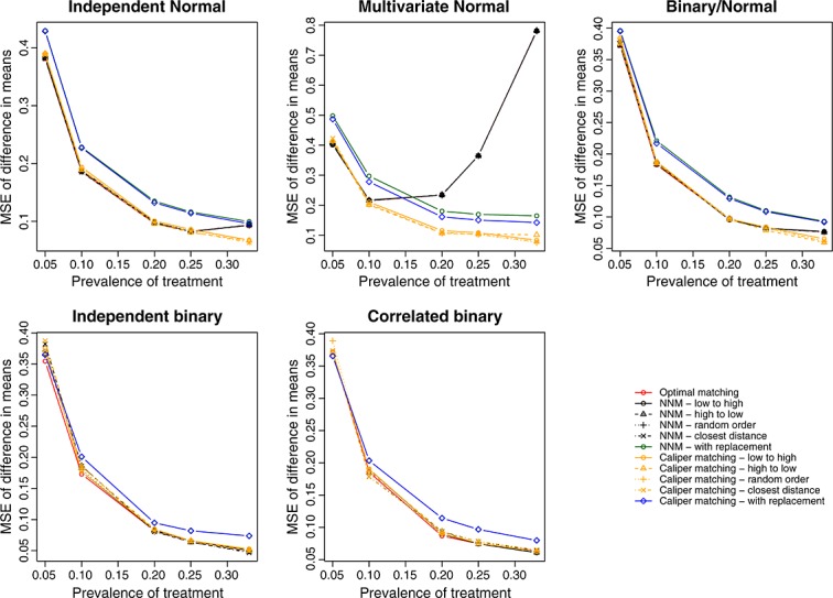
Treatment effect: mean squared error of difference in means.
Figure 5.
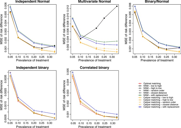
Treatment effect: mean squared error of risk difference.
We report the mean absolute standardized differences for the 10 covariates under the different matching algorithms in Figures A4–A8 in the Supporting information for the five different sets of distributions for the baseline covariates. Several observations merit comment. First, in a few of the scenarios, matching with replacement resulted in slightly greater imbalance in measured baseline covariates compared with matching without replacement. This finding at first appears counterintuitive, because matching with replacement matches each treated subject to the nearest untreated subject. Thus, one would expect better balance on baseline covariates compared with the competing approaches. However, this finding is a result of how balance is assessed. Matching with replacement will most likely result in the same untreated subject being included multiple times in the matched sample. Thus, when the variance of the baseline covariate is estimated in treated and untreated subjects, the inclusion of the same untreated subject in multiple matched pairs will reduce the variability of the baseline covariate in the matched untreated subjects. This will result in an inflation of the standardized difference, because the pooled variance of the baseline covariate forms the denominator of the standardized difference. Second, when at least some of the baseline covariates were normally distributed, caliper matching without replacement tended to result in improved balance compared with methods based on nearest neighbor matching without replacement. The differences between these two sets of algorithms increased as the proportion of subjects who were treated increased. Third, optimal matching and the different implementations of nearest neighbor matching without replacement tended to result in the same balance in baseline covariates across the different scenarios.
We conducted a brief, post-hoc analysis to examine the stability of our findings due to the use of 1000 simulated datasets. We restricted our attention to one scenario (multivariate normal covariates and a prevalence of exposure of 5%) and one method (caliper matching—random order). In this sensitivity analysis, we replicated our simulations 10 times—we created 1000 simulated datasets 10 times. We constructed each of the 10,000 simulated datasets using a different random number seed. We then determined the mean estimated treatment effect and the MSE of the estimated treatment effect in each of the 10 sets of 1000 simulated datasets. When using caliper matching (random order), the estimated difference in means ranged from 0.980 to 1.033 across the 10 sets of simulated datasets, whereas the MSE of the estimate ranged from 0.384 to 0.440. Similarly, the estimated mean risk difference ranged from − 0.022 to − 0.013, whereas the MSE of the estimate ranged from 0.0067 to 0.0074.
4 Case study
We used a sample of 9107 patients discharged from 103 acute care hospitals in Ontario, Canada, with a diagnosis of AMI (or heart attack) between April 1, 1999 and March 31, 2001. We collected data on these subjects as part of the Enhanced Feedback for Effective Cardiac Treatment (EFFECT) study, an initiative intended to improve the quality of care for patients with cardiovascular disease in Ontario 13,14. The EFFECT study consisted of two phases. We collected data on patient demographics, vital signs and physical examination at presentation, medical history, and results of laboratory tests for this sample.
For the current case study, the exposure of interest was whether the patient received a prescription for a statin lipid-lowering agent at hospital discharge. Three thousand and forty-nine (33.5%) patients received a prescription at hospital discharge. The outcome of interest for this case study was a binary variable denoting whether the patient died within 8 years of hospital discharge. Three thousand five hundred and ninety-three (39.5%) patients died within 8 years of hospital discharge. Additional propensity score analyses in this sample are described elsewhere 20,21.
We estimated a propensity score for statin treatment using logistic regression to regress an indicator variable denoting statin treatment on 30 baseline covariates. We used restricted cubic smoothing splines to model the relationship between each of the 11 continuous covariates and the log-odds of statin prescribing. We used each of the matching algorithms described earlier to form matched samples consisting of pairs of treated and untreated subjects.
Figure 6 reports the standardized difference for each of the 30 baseline covariates in the original, unmatched sample and in each of the matched samples. In the original sample, 10 of the 30 covariates had standardized differences that exceeded 0.10, with the largest standardized difference being for history of hyperlipidemia (0.88). Optimal matching and the nearest neighbor matching without replacement algorithms resulted in substantially improved balance. In the matched samples, 29 of the 30 covariates had standardized differences that were less than 0.10. The standardized difference for hyperlipidemia remained large (0.43) in these matched samples. The four algorithms based on caliper matching without replacement resulted in substantial reductions in imbalance: all standardized differences were less than 0.101. Of these algorithms, caliper matching (closest distance) resulted in the best balance (all standardized differences were less than 0.04).
Figure 6.
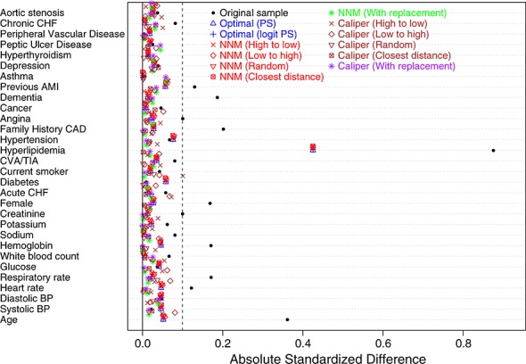
Balance of baseline covariates between treated/untreated subjects.
Figure 7 reports the absolute reductions in the probability of death within 8 years of discharge. The crude reduction in the probability of death was 0.154. The two optimal matching algorithms and the four greedy nearest neighbor matching algorithms that used matching without replacement resulted in similar estimates of the absolute risk reduction (0.021 to 0.023). We observed greater variability for caliper matching without replacement (0.017 to 0.058). The most disparate estimate (0.058) was caliper matching (high to low))
Figure 7.

Estimated absolute risk reduction.
5 Discussion
We used a series of Monte Carlo simulations to examine the relative performance of different algorithms for forming pairs of treated and untreated subjects matched on the propensity score. In this section, we briefly summarize our findings and place them in the context of the prior literature.
We made several important observations in our Monte Carlo simulations. First, because optimal and nearest neighbor matching result in a matched sample with a larger number of matched pairs, the use of these algorithms tended to result in estimates with greater precision compared with when caliper matching was used (i.e., we observed a smaller variation in the estimated treatment effects across the simulated samples). Second, because nearest neighbor matching within specified caliper widths imposes a maximum difference in propensity scores between treated and untreated subjects within a matched pair, it tended to result in less biased estimates compared with the other matching algorithms. Third, as a result of the aforementioned two observations, the choice between caliper matching and optimal or nearest neighbor matching reflects the variance-bias trade-off. Fourth, using MSE, caliper matching without replacement tended to have a performance that was at least as good as any of the competing algorithms. Fifth, for both caliper matching without replacement and nearest neighbor matching without replacement, we examined whether the order in which treated subjects were sequentially selected for matching had an impact on estimation. Although none of the orderings (low to high, high to low, closest distance, or random) had uniformly superior performance in terms of bias, sequentially selecting treated subjects from highest to lowest propensity score tended to result in greater bias compared with the other three methods of selecting subjects. Similarly, no method of sequentially selecting treated subjects was clearly optimal compared with the others when examining the MSE of the treatment effect. Finally, when comparing optimal matching with the four variants of nearest neighbor matching without replacement, in the majority of scenarios examined, nearest neighbor matching with random selection of treated units resulted in estimates of effect with MSE that was at least as low as that obtained using optimal matching.
Optimal matching and nearest neighbor matching both result in all treated subjects being included in the matched sample. However, nearest neighbor matching within specified calipers can result in the exclusion of some treated subjects from the matched sample if there are insufficient untreated subjects with a propensity score near that of some of the treated subjects. Rosenbaum and Rubin used the term ‘bias due to incomplete matching’ to describe the bias that arises when treated subjects are excluded from the matched sample 9. Matching allows one to estimate the effect of treatment in those subjects who are ultimately treated. If some treated subjects are excluded from the matched sample, then it is unclear to what treated population the estimated treatment effect applies. This may limit the generalizability of the estimated effect and the ability to describe the population to which it pertains. The use of optimal and nearest neighbor matching avoids bias due to incomplete matching but at the expense of greater bias in the estimated treatment effect.
Despite the observation that no method of selecting the treated subjects for matching had clearly superior performance to the other selection methods, we would recommend that, for conceptual reasons, random selection of treated units be used, particularly when using caliper matching. Matching allows one to estimate the ATT: the effect of treatment in treated subjects. When using caliper matching, some untreated subjects are often excluded from the final matched sample. We hypothesize that random selection of treated units will result in a final matched sample in which the matched treated subjects are most similar to a random sample from the set of all treated subjects. This may improve generalizability and reduce bias due to incomplete matching.
The current study is, to the best of our knowledge, the first to compare matching algorithms based on matching with replacement with other commonly-used matching algorithms. On the basis of our findings, we would discourage the use of matching with replacement when forming propensity-score matched samples. Matching with replacement did not result in estimates with less bias compared with the best-performing methods based on caliper matching without replacement. Furthermore, matching with replacement resulted in estimates that displayed greater variability and that had higher MSE compared with estimates obtained using caliper matching without replacement. Although we estimated the variability of the estimated treatment effects across the 1000 simulated datasets for each scenario, estimating the standard error of an estimated treatment effect obtained using matching with replacement requires specialized methods. Methods for this have been described when the outcome is continuous 22. However, comparable methods have not been described for settings with binary outcomes.
There is a paucity of research comparing different matching algorithms. Ming and Rosenbaum examined improvements in bias reduction when a variable number of controls were matched to each treated subject compared with when a fixed number of controls were used 23. They found that variable matching can result in substantial improvements in bias reduction at the cost of only a minor increase in variance. Gu and Rosenbaum compared optimal matching with nearest neighbor matching 24. Our findings were comparable to theirs: optimal matching resulted in matched pairs in which the mean difference in the propensity score was less than when nearest neighbor matching was used. However, optimal matching did not result in improved balance in measured baseline covariates. Gu and Rosenbaum restricted their attention to covariate balance and differences in the propensity score. The current study complements their study by examining estimation of treatment effects (both differences in means and risk differences) and reporting bias, variance, and MSE. Apart from these earlier studies, there is a dearth of studies comparing the performance of different matching algorithms.
There are certain limitations to the current study that bear noting. First, the focus was on methods for pair-matching on the propensity score. We did not consider full matching nor methods for matching multiple untreated or controls subject to each treated subject. We focused on methods for forming pairs of treated and untreated subjects as this is the most common implementation of propensity score matching in the applied literature 4. Although applied investigators have occasionally matched multiple untreated subjects to each treated subject, it is rarely optimal to include more than two untreated subjects per treated subject 25. A second limitation is that we only considered one caliper width when using nearest neighbor matching within a specified caliper width (0.2 of the standard deviation of the logit of the propensity score). This caliper width was selected as it has been shown to be optimal when estimating differences in means and risk differences in a variety of settings 11. To simplify the simulations and the presentation of the results, we did not consider a range of calipers in the current study. Third, our findings were based on Monte Carlo simulations and thus require replication under a variety of data-generating processes. However, we would note that our extensions were extensive, and we examined five different sets of distributions for the baseline covariates. Fourth, for nearest neighbor matching, we examined matching on the propensity score, whereas for nearest neighbor caliper matching, we examined matching on the logit of the propensity score. This was to reflect how these methods are commonly used in practice. To have examined matching on both metrics for each method would have made the results difficult to present, because there would have been 22 different algorithms, rather than the 12 that we examined. For optimal matching, we examined matching on the propensity score and on the logit of the propensity score. These two different implementations of optimal matching resulted in identical results. Thus, we suspect that the choice of whether to match on the propensity score or on the logit of the propensity may have at most a modest impact on the performance of the different algorithms.
In the methodological literature, researchers have conducted substantial research on methods to estimate effects using propensity-score methods. However, they have given relatively little attention to comparing the methods used for forming pairs of subjects matched on the propensity score. The current study addresses this gap in the existing literature and provides important information as to how best to implement propensity-score matching.
In conclusion, we would recommend that, in most situations, nearest neighbor caliper matching without replacement (random order or closest distance) be used when forming pairs of treated and untreated subjects with similar values of the propensity score. These two approaches tended to result in estimates with minimal bias compared with the other algorithms across a wide range of scenarios. Furthermore, the use of either of these two algorithms resulted in estimates that displayed only negligibly greater variability than the nearest neighbor matching algorithms, which tended to have the best performance. Finally, these two algorithms resulted in estimates that had amongst the lowest MSE.
Acknowledgments
The Institute for Clinical Evaluative Sciences (ICES) supported this study, which is funded by an annual grant from the Ontario Ministry of Health and Long-Term Care (MOHLTC). The opinions, results, and conclusions reported in this paper are those of the authors and are independent from the funding sources. No endorsement by ICES or the Ontario MOHLTC is intended or should be inferred. In part, a Career Investigator award from the Heart and Stroke Foundation of Ontario supported Dr. Austin. In part, an operating grant from the Canadian Institutes of Health Research (CIHR) (Funding number: MOP 86508) supported this study. The CIHR Team Grant in Cardiovascular Outcomes Research funded the EFFECT study. These data sets used for analysis were held securely in a linked, de-identified form and analyzed at the Institute for Clinical Evaluative Sciences.
Supporting Information
Supporting info item
References
- Rosenbaum PR, Rubin DB. The central role of the propensity score in observational studies for causal effects. Biometrika. 1983;70:41–55. [Google Scholar]
- Rosenbaum PR. Model-based direct adjustment. Journal of the American Statistical Association. 1987;82:387–394. [Google Scholar]
- Austin PC. Propensity-score matching in the cardiovascular surgery literature from 2004 to 2006: a systematic review and suggestions for improvement. Journal of Thoracic and Cardiovascular Surgery. 2007;134(5):1128–1135. doi: 10.1016/j.jtcvs.2007.07.021. [DOI] [PubMed] [Google Scholar]
- Austin PC. A critical appraisal of propensity-score matching in the medical literature between 1996 and 2003. Statistics in Medicine. 2008;27(12):2037–2049. doi: 10.1002/sim.3150. [DOI] [PubMed] [Google Scholar]
- Thoemmes FJ, Kim ES. A systematic review of propensity score methods in the social sciences. Multivariate Behavioral Research. 2011;46(1):90–118. doi: 10.1080/00273171.2011.540475. [DOI] [PubMed] [Google Scholar]
- Austin PC. A report card on propensity-score matching in the cardiology literature from 2004 to 2006: a systematic review and suggestions for improvement. Circulation: Cardiovascular Quality and Outcomes. 2008;1:62–67. doi: 10.1161/CIRCOUTCOMES.108.790634. [DOI] [PubMed] [Google Scholar]
- Imbens GW. Nonparametric estimation of average treatment effects under exogeneity: a review. Review of Economics and Statistics. 2004;86:4–29. [Google Scholar]
- Rosenbaum PR. Observational Studies. New York, NY: Springer-Verlag; 2002. [Google Scholar]
- Rosenbaum PR, Rubin DB. Constructing a control group using multivariate matched sampling methods that incorporate the propensity score. The American Statistician. 1985;39:33–38. [Google Scholar]
- Austin PC. Some methods of propensity-score matching had superior performance to others: results of an empirical investigation and Monte Carlo simulations. Biometrical Journal. 2009;51(1):171–184. doi: 10.1002/bimj.200810488. [DOI] [PubMed] [Google Scholar]
- Austin PC. Optimal caliper widths for propensity-score matching when estimating differences in means and differences in proportions in observational studies. Pharmaceutical Statistics. 2011;10:150–161. doi: 10.1002/pst.433. [DOI] [PMC free article] [PubMed] [Google Scholar]
- Cochran WG, Rubin DB. Controlling bias in observational studies: a review. Sankhya: The Indian Journal of Statistics. 1973;35:416–466. [Google Scholar]
- Tu JV, Donovan LR, Lee DS, Wang JT, Austin PC, Alter DA, Ko DT. Effectiveness of public report cards for improving the quality of cardiac care: the EFFECT study: a randomized trial. Journal of the American Medical Association. 2009;302(21):2330–2337. doi: 10.1001/jama.2009.1731. [DOI] [PubMed] [Google Scholar]
- Tu JV, Donovan LR, Lee DS, Austin PC, Ko DT, Wang JT, Newman AM. Toronto, Ontario: 2004. Quality of cardiac care in Ontario, Institute for Clinical Evaluative Sciences: [Google Scholar]
- Austin PC. A data-generation process for data with specified risk differences or numbers needed to treat. Communications in Statistics - Simulation and Computation. 2010;39:563–577. DOI: 10.1080/03610910903528301. [Google Scholar]
- Sturmer T, Joshi M, Glynn RJ, Avorn J, Rothman KJ, Schneeweiss S. A review of the application of propensity score methods yielded increasing use, advantages in specific settings, but not substantially different estimates compared with conventional multivariable methods. Journal of Clinical Epidemiology. 2006;59(5):437–447. doi: 10.1016/j.jclinepi.2005.07.004. [DOI] [PMC free article] [PubMed] [Google Scholar]
- Austin PC, Grootendorst P, Anderson GM. A comparison of the ability of different propensity score models to balance measured variables between treated and untreated subjects: a Monte Carlo study. Statistics in Medicine. 2007;26(4):734–753. doi: 10.1002/sim.2580. [DOI] [PubMed] [Google Scholar]
- Flury BK, Riedwyl H. Standard distance in univariate and multivariate analysis. The American Statistician. 1986;40:249–251. [Google Scholar]
- Austin PC. Balance diagnostics for comparing the distribution of baseline covariates between treatment groups in propensity-score matched samples. Statistics in Medicine. 2009;28(25):3083–3107. doi: 10.1002/sim.3697. [DOI] [PMC free article] [PubMed] [Google Scholar]
- Austin PC. A tutorial on the use of propensity scoremethods with survival or time-to-event outcomes: Reporting measures of effect similar to those used in randomized experiments. Statistics in Medicine. doi: 10.1002/sim.5984. In press. DOI: 10.1002/sim.5984. [DOI] [PMC free article] [PubMed] [Google Scholar]
- Austin PC, Mamdani MM. A comparison of propensity scoremethods: A case-study estimating the effectiveness of post-AMI statin use. Statistics in Medicine. 2006;25:2084–2106. doi: 10.1002/sim.2328. DOI: 10.1002/sim.2328. [DOI] [PubMed] [Google Scholar]
- Hill J, Reiter JP. Interval estimation for treatment effects using propensity score matching. Statistics in Medicine. 2006;25(13):2230–2256. doi: 10.1002/sim.2277. [DOI] [PubMed] [Google Scholar]
- Ming K, Rosenbaum PR. Substantial gains in bias reduction from matching with a variable number of controls. Biometrics. 2000;56(1):118–124. doi: 10.1111/j.0006-341x.2000.00118.x. [DOI] [PubMed] [Google Scholar]
- Gu XS, Rosenbaum PR. Comparison of multivariate matching methods: structures, distances, and algorithms. Journal of Computational and Graphical Statistics. 1993;2:405–420. [Google Scholar]
- Austin PC. Statistical criteria for selecting the optimal number of untreated subjects matched to each treated subject when using many-to-one matching on the propensity score. American Journal of Epidemiology. 2010;172(9):1092–1097. doi: 10.1093/aje/kwq224. [DOI] [PMC free article] [PubMed] [Google Scholar]
Associated Data
This section collects any data citations, data availability statements, or supplementary materials included in this article.
Supplementary Materials
Supporting info item