Interpreting observational studies: why empirical calibration is needed to correct p-values

Abstract

Often the literature makes assertions of medical product effects on the basis of ‘ p < 0.05’. The underlying premise is that at this threshold, there is only a 5% probability that the observed effect would be seen by chance when in reality there is no effect. In observational studies, much more than in randomized trials, bias and confounding may undermine this premise. To test this premise, we selected three exemplar drug safety studies from literature, representing a case–control, a cohort, and a self-controlled case series design. We attempted to replicate these studies as best we could for the drugs studied in the original articles. Next, we applied the same three designs to sets of negative controls: drugs that are not believed to cause the outcome of interest. We observed how often p < 0.05 when the null hypothesis is true, and we fitted distributions to the effect estimates. Using these distributions, we compute calibrated p-values that reflect the probability of observing the effect estimate under the null hypothesis, taking both random and systematic error into account. An automated analysis of scientific literature was performed to evaluate the potential impact of such a calibration. Our experiment provides evidence that the majority of observational studies would declare statistical significance when no effect is present. Empirical calibration was found to reduce spurious results to the desired 5% level. Applying these adjustments to literature suggests that at least 54% of findings with p < 0.05 are not actually statistically significant and should be reevaluated. © 2013 The Authors. Statistics in Medicine published by John Wiley & Sons Ltd.

1. Introduction

Observational studies deliver an increasingly important component of the evidence base concerning the effects of medical products. Payers, regulators, providers, and patients actively employ observational studies in therapeutic decision making. While randomized controlled trials (RCTs) are regarded as the gold standard of evidence when measuring treatment effects, conducting these experiments remains resource intensive, time consuming, can suffer from limitations in sample size and generalizability, and often may be infeasible or unethical to implement. In contrast, the non-interventional secondary use of observational data collected within the healthcare system for purposes such as reimbursement or for clinical care can yield timely and cost-efficient insights about real-world populations and current treatment behaviors at a small fraction of the cost and in days instead of years. With these potential advantages comes the recognition that observational studies can suffer from various biases and that results might not always be reliable. Results from observational studies often cannot be replicated ^1,2. For example, two recent independent observational studies investigating oral bisphosphonates and the risk of esophageal cancer produced results leading to conflicting conclusions ^3,4, despite the fact that the two studies analyzed the same database over approximately the same period. A systematic analysis has suggested that the majority of observational studies return erroneous results ⁵. The main source of these problems is that observational studies are more vulnerable than RCTs to systematic error such as bias and confounding. In RCTs, randomization of the exposure helps to ensure that exposed and unexposed populations are comparable. Observational studies, by definition, merely observe clinical practice, and exposure is no longer the only potential explanation for observed differences in outcomes. Many statistical methods exist that aim to reduce this systematic error, including self-controlled designs ⁶ and propensity score adjustment ⁷, but it is unclear to what extent these solve the problem.

Despite the fact that the problem of residual systematic error is widely acknowledged (often in the discussion section of articles), the results are sometimes misinterpreted as if this error did not exist. Most important, statistical significance testing, which only accounts for random error, is widely used in observational studies. Significance tests compute the probability that a study finding at least as extreme as the one reported could have arisen under the null hypothesis (usually the hypothesis of no effect). This probability, called the p-value, is compared against a predefined threshold α (usually 0.05), and if p < α, the finding is deemed to be ‘statistically significant’.

Although we believe that most researchers are aware of the fact that traditional p-value calculations do not adequately take systematic error into account, likely because of a lack of a better alternative, the notion of statistical significance based on the traditional p-value is widespread in the medical literature. Using PubMed, we conducted a systematic review of this literature in the last 10 years and identified 4970 observational studies exploring medical treatment with effect estimates in their abstracts. Of these, 1362 provided p-values in the abstract, and 83% of these p-values indicated statistical significance. The remaining 3608 articles provided 95% confidence intervals instead. Of these confidence intervals, 82% excluded 1 and therefore also indicated statistical significance. The details of this analysis are provided in the Supporting information, Appendix F^‡.

In this research, we focus on the fundamental notion of statistical significance in observational studies, testing the degree to which observational analyses generate significant findings in situations where no association exists. To accomplish this, we selected two publications: one investigating the relationship between isoniazid and acute liver injury ⁸ and one investigating sertraline and upper gastrointestinal (GI) bleeding ⁹. These two publications represent three popular study designs in observational research: the first publication used a cohort design, and the second paper used both a case–control design and a self-controlled case series (SCCS). We replicated these studies as best we could, closely following the specific design choices. However, because we did not have access to the same data, we used suitable substitute databases. For each study, we identified a set of negative controls (drug–outcome pairs for which we have confidence that there is no causal relationship) and explored the performance of the study designs. We show that the designs frequently yield biased estimates, misrepresent the p-value, and lead to incorrect inferences about rejecting the null hypothesis. We introduce a new empirical framework, based on modeling the observed null distribution for the negative controls that yields properly calibrated p-values for observational studies. Using this approach, we observe that about 5% of drug–outcome negative controls have p < 0.05, as is expected and desired. By applying this framework to a large set of historical effect estimates under various assumptions of bias, we show that for the majority of estimates currently considered statistically significant, we would not be able to reject the null hypothesis after calibration. Our framework provides an explicit formula for estimating the calibrated p-value using the traditionally estimated relative risk and standard error. As such, all stakeholders can easily employ this decision tool as an aid for minimizing the potential effects of bias when interpreting observational study results.

2. Methods

2.1. Example study 1: Isoniazid and acute liver injury using a cohort design

Smith et al. ⁸ used administrative health data from the province of Quebec to investigate the relationship (odds ratio) between tuberculosis treatment (mostly isoniazid) and hepatic events in a cohort design study. We conducted a similar study in the Thomson MarketScan Medicare Supplemental Beneficiaries database, which contains data on 4.6 million subjects. We selected two groups (cohorts): (1) all subjects exposed to isoniazid and (2) all subjects having the ailment for which isoniazid is indicated, in this case tuberculosis, and having received at least one drug that is not known to cause acute liver injury. We removed all subjects who belonged to both groups and subjects for which less than 180 days of observation time was available prior to their first exposure to the drug in question. Acute liver injury was identified on the basis of the occurrence of ICD-9-based diagnosis codes from inpatient and outpatient medical claims and was defined broadly on the basis of codes associated with hepatic dysfunction, as have been used in prior observational database studies ^10–13 The full list of codes is provided in the Supporting information, Appendix A. The time at risk was defined as the length of exposure + 30 days, and we determined whether subjects experienced an acute liver injury during their time at risk. Using propensity score stratification, the cohorts were divided over 20 strata, and an odds ratio over all strata was computed using a Mantel–Haenszel test. The propensity score was estimated using Bayesian logistic regression using all available drug, condition, and procedure covariates occurring in the 180 days prior to first exposure, in addition to age, sex, calendar year of first exposure, Charlson index, number of drugs, number of visit days, and number of procedures.

2.2 Example study 2: SSRIs and upper GI bleeding using a case–control design

Tata et al. ⁹ conducted a case–control analysis using a database of computerized medical records from general practices across England and Wales to study the relationship (odds ratio) between selective serotonin reuptake inhibitors (SSRIs) and upper GI bleeding. We used a comparable database of medical records from general practices in the USA, the General Electric (GE) Centricity database, which contains data on 11.2 million subjects. We used similar restrictions on study period (start of 1990 through November 2003), age requirements (18 years or older), available time prior to event (180 days), number of controls per case (6), and risk definition window (30 days following the prescription). Controls were matched on age and sex but not on postal code because these data were not readily available in our database. Instead of considering several SSRIs, we selected a single drug: sertraline. Cases of upper GI bleeding were identified on the basis of the occurrence of ICD-9 diagnosis codes in the problem list. These codes pertain to esophageal, gastric, duodenal, peptic, and gastrojejunal ulceration, perforation, and hemorrhage, as well as gastritis and non-specific gastrointestinal hemorrhage, and have previously been evaluated through source record verification ^14–16. The full list of codes is provided in the Supporting information, Appendix A.

2.3. Example study 3: SSRIs and upper GI bleeding using an SCCS design

To check the robustness of their findings, Tata et al. ⁹ also conducted an SCCS to estimate the incidence rate ratio using the same data. Again, we used the GE Centricity database and duplicated the study design choices, including the removal of the 30 days prior to the first prescription as introduced by the authors to account for possible contraindications.

2.4. Selection of negative controls

For our negative controls, we could either pick different drugs that are known not to cause the outcome of interest or pick outcomes that are known not to be caused by our drug of interest ¹⁷. Picking different outcomes would be more difficult in observational studies because some study designs such as case–control are focused on outcomes and would require resampling of subjects and because outcomes are often more difficult to extract from observational data, requiring complex algorithms that need to be validated. On the other hand, different drug exposures are usually easily and fairly accurately identified in prescription tables, and we therefore have opted for using negative control drugs.

We focus our analysis on the two outcomes in our example studies: acute liver injury and upper GI bleeding. Both outcomes arise frequently in drug safety studies. We attempted to perform an exhaustive search to define exposure controls for these two outcomes by starting with all drugs with an active structured product label. Subsequently, we selected only those drugs meeting the following criteria:

1. The outcome of interest could not be listed in any section of the Food and Drug Administration structured product label, nor could any related outcome be listed.

2. The drug could not be listed as a ‘causative agent’ for the outcome in the book Drug-Induced Diseases: Prevention, Detection and Management [18].

3. A manual review of the literature found no studies showing the drug caused the outcome.

For acute liver injury, we found 37 negative controls, while for upper GI bleeding, 67 drugs met these criteria. Appendix B (Supporting information) provides the full list.

2.5. Effect of confounding by indication

Arguably, when certain types of bias are expected to be present when designing a study, one might reject certain design choices for that reason. For example, a case–control design is deemed by some to be less appropriate when confounding by indication is considered likely because of limited options to adjust for this type of confounding. Instead, one would perhaps opt for a cohort design and restrict the comparator population to those also having the ailment for which the drug of interest is indicated and use propensity score adjustment, or choose a self-controlled design such as the SCCS. To estimate whether this ‘informed design’ would change the observed distribution, we refitted the distribution for the case–control design while eliminating control drugs with obvious potential for confounding by indication: amylases, endopeptidases, hyoscyamine, and sucralfate are all drugs for the treatment of peptic ulcers and are therefore more likely to be observed when studying upper GI bleeds, while epoetin alfa and ferrous gluconate are two drugs that are used to combat anemia, one of the possible consequences of upper GI bleeding.

2.6. Calibrating p-values

Traditional significance testing utilizes a theoretical null distribution that requires a number of assumptions to ensure its validity. Our proposed approach instead derives an empirical null distribution from the actual effect estimates for the negative controls. These negative control estimates give us an indication of what can be expected when the null hypothesis is true, and we use them to estimate an empirical null distribution. We fitted a Gaussian probability distribution to the estimates, taking into account the sampling error of each estimate. We have found that a Gaussian distribution provides a good approximation, and more complex models, such as mixtures of Gaussians and non-parametric density estimation, did not improve results. Let y_i denote the estimated log effect estimate (relative risk, odds or incidence rate ratio) from the ith negative control drug–outcome pair, and let τ_i denote the corresponding estimated standard error, i = 1,…,n. Let θ_i denote the true (but unknown) bias associated with pair i, that is, the log of the effect estimate that the study for pair i would have returned had it been infinitely large. As in the standard p-value computation, we assume that y_i is normally distributed with mean θ_i and standard deviation τ_i. Note that in traditional p-value calculation, θ_i is always assumed to be equal to zero, but that we assume the θ_i′s, arise from a normal distribution with mean μ and variance σ². This represents the null (bias) distribution. We estimate μ and σ² via maximum likelihood. In summary, we assume the following:

where N(a, b) denotes a Gaussian distribution with mean a and variance b, and estimate μ and σ² by maximizing the following likelihood:

We compute a calibrated p-value that uses the empirical null distribution. Let y_n + 1 denote the log of the effect estimate from a new drug–outcome pair, and let τ_n + 1 denote the corresponding estimated standard error. From the aforementioned assumptions and assuming θ_n + 1 arises from the same null distribution, we have the following:

When y_n + 1 is smaller than , the one sided p-value for the new pair is then

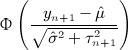where Φ( • ) denotes the cumulative distribution function of the standard normal distribution. When y_n + 1 is bigger than , the one sided p-value is then

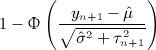Throughout the paper, we have converted these to a single two-sided p-value by taking the lowest of the upper and lower bound p-value and multiply it by 2. The R-code for estimating the null distribution and calibrating the p-value can be found in the Supporting information, Appendix D.

3. Results

Our replication of the published studies produced similar results. The original cohort study reported an odds ratio of 6.4 (95% CI 2.2–18.3, p < 0.001) for isoniazid and acute liver injury, compared with an odds ratio of 4.0 (95% CI 2.7–6.0, p < 0.001) found in our reproduction. In total, we identified 2807 subjects that were exposed to the drug, for a total of 384,659 days. In the whole population cover by the database, 264,122 subjects met our criteria for acute liver injury.

The original case–control study reported an odds ratio of 2.4 (95% CI 2.1–2.7, p < 0.001) for sertraline and upper GI bleeding, while our reproduction yielded an odds ratio of 2.2 (95% CI 1.9–2.5, p < 0.001). The original self-controlled case study of the same relationship reported an incidence rate ratio of 1.7 (95% CI 1.5–2.0, p < 0.001) compared with an incidence rate ratio of 2.1 (95% CI 1.8–2.4, p < 0.001) found in our reproduction. In total, 441,340 subjects were exposed to sertraline for a total duration of 108,759,375 days. In the entire database, 108,882 subjects met our criteria for upper GI bleeding.

3.1. Distribution of negative controls

We applied the three study designs to the negative controls for the respective health outcomes of interest.

Figure 1 shows the estimated odds ratios and incidence rate ratios, which can also be found in tabular form in the Supporting information, Appendix C. For the case–control and SCCS designs, applying the same study design to other drugs was straightforward. For the cohort method, most drugs had different comparator groups of patients and required recomputing propensity scores. For three of the negative controls for acute liver injury and 23 of the negative controls for upper GI bleeding, there were not enough data to compute an estimate, for instance, because none of the cases and none of the controls were exposed to the drug. However, an initial investigation in the minimum number of required controls showed the remaining number sufficed (Supporting information, Appendix E). Note that the number of exposed subjects varies greatly from drug to drug, from 67 subjects being exposed to neostigmine to 884,644 individuals having exposure to fluticasone (Supporting information, Appendix C). These differences account for the majority in variation of the widths of the confidence intervals.

Figure 1.

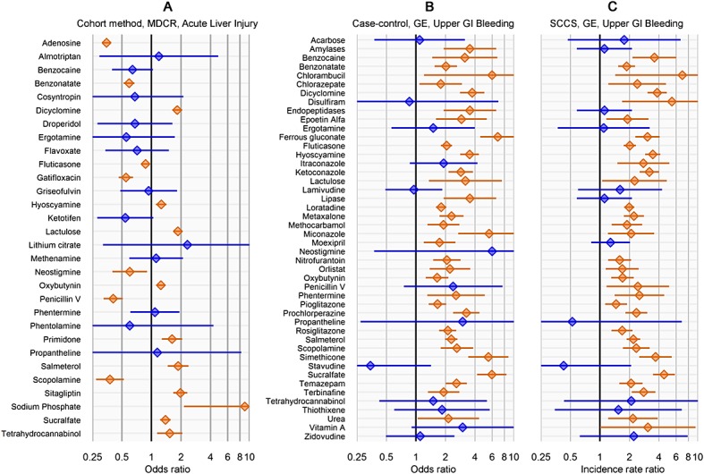
Forest plots of negative controls. Lines show 95% confidence interval. Orange indicates statistically significant estimates (two-sided p < 0.05), and blue indicates non-significant estimates.

From Figure 1, it is clear that traditional significance testing fails to capture the diversity in estimates that exists when the null hypothesis is true. Despite the fact that all the featured drug–outcome pairs are negative controls, a large fraction of the null hypotheses are rejected. We would expect only 5% of negative controls to have p < 0.05. However, in Figure 1A (cohort method), 17 of the 34 negative controls (50%) are either significantly protective or harmful. In Figure 1B (case–control), 33 of 46 negative controls (72%) are significantly harmful. Similarly, in Figure 1C (SCCS), 33 of 46 negative controls (72%) are significantly harmful, although not the same 33 as in Figure 1B.

These numbers cast doubts on any observational study that would claim statistical significance using traditional p-value calculations. Consider, for example, the odds ratio of 2.2 that we found for sertraline using the case–control method, we see in Figure 1B that many of the negative controls have similar or even higher odds ratios. The estimate for sertraline was highly significant (p < 0.001), meaning the null hypothesis can be rejected on the basis of the theoretical model. However, on the basis of the empirical distribution of negative controls, we can argue that we cannot reject the null hypothesis so readily.

3.2. Calibration of p-values

Using the empirical distributions of negative controls, we can compute a better estimate of the probability that a value at least as extreme as a certain effect estimate could have been observed under the null hypothesis. For the three designs we considered, Table 1 provides the maximum likelihood estimates for the means and variances of the empirical null distributions. Interestingly, in our study, while the cohort method has nearly zero bias on average, the case–control and SCCS methods are positively biased on average. It is important to note that for all three designs, is not equal to zero, meaning that the bias in an individual study may deviate considerably from the average.

Table 1.

Estimated mean and variance of the empirical null distribution for the three study designs.

Design
Cohort	− 0.05	0.54
Case–control	0.90	0.35
SCCS	0.79	0.28

When eliminating the six drugs where we expect confounding by indication, the estimated parameters for the case–control design change slightly to and .

Figure 2 shows for every level of α the fraction of negative controls for which the p-value is below α, for both the traditional p-value calculation and the calibrated p-value using the empirically established null distribution. For the calibrated p-value, a leave-one-out design was used: for each negative control, the null distribution was estimated using all other negative controls. A well-calibrated p-value calculation should follow the diagonal: for negative controls, the proportion of estimates with p < α should be approximately equal to α. Most significance testing uses an α of 0.05, and we see in Figure 2 that the calibrated p-value leads to the desired level of rejection of the null hypothesis. For the cohort method, case–control, and SCCS, the number of significant negative controls after calibration is 2 of 34 (6%), 5 of 46 (11%), and 3 of 46 (5%), respectively.

Figure 2.

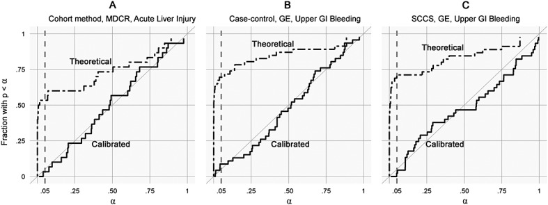
Calibration plots. Each subplot shows the fraction of negative controls with p < α, for different levels of α. Both traditional p-value calculation and p-values using calibration are shown. For the calibrated p-value, a leave-one-out design was used.

Applying the calibration to our three example studies, we find that only the cohort study of isoniazid reaches statistical significance: p = 0.01. The case–control and SCCS analysis of sertraline produced p-values of 0.71 and 0.84, respectively.

3.3. Visualization of the calibration

A graphical representation of the calibration is shown in Figure 3. By plotting the effect estimate on the x-axis and the standard error of the estimate on the y-axis, we can visualize the area where the traditional p-value is smaller than 0.05 (the gray area below the dashed line) and where the calibrated p-value is smaller than 0.05 (orange area). Many of the negative controls (blue dots) fall within the gray area indicating traditional p < 0.05, but only a few fall within the orange area indicating a calibrated p < 0.05.

Figure 3.

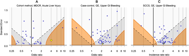
Traditional and calibrated significance testing. Estimates below the dashed line (gray area) have p < 0.05 using traditional p-value calculation. Estimates in the orange areas have p < 0.05 using the calibrated p-value calculation. Blue dots indicate negative controls, and the yellow diamond indicates the drugs of interest: isoniazid (A) and sertraline (B and C).

In Figure 3A, the drug of interest isoniazid (yellow diamond) is clearly separated from the negative controls, and this is the reason we feel confident we can reject the null hypothesis of no effect. In Figure 3B and C, the drug of interest sertraline is indistinguishable from the negative controls. These studies provide little evidence for rejecting the null hypothesis.

3.4. Literature analysis

The medical literature features many observational studies that use traditional significance testing to assert whether an effect was observed. Assuming that these studies have similar null distributions as our three example studies, we can test whether for historical significant findings, we can still reject the null hypothesis after calibration. Using an elaborate PubMed query (Supporting information, Appendix F), we identified 31,386 papers published in the last 10 years that applied a cohort, case–control, or SCCS design in a study using observational healthcare data. Through an automated text-mining procedure, we extracted 4970 articles where a relative risk, hazard, odds, or incidence rate ratio estimate was mentioned in the abstract. These estimates were accompanied by either a p-value or a confidence interval, and we used these to back calculate the standard error, allowing us to recompute the calibrated p-value under various assumptions of bias. The full list of estimates and recomputed p-values can be found in the Supporting information, Appendix G.

Figure 4 shows the number of estimates per publication year. The vast majority of these estimates (82% of all estimates) are statistically significant under the traditional assumption of no bias. But even with the most modest assumption of bias (mean  =  0, SD  =  0.25), this number dwindles to less than half (38% of all estimates). This suggests that at least 54% of significant findings would be deemed non-significant after calibration. With an assumption of medium size bias (mean  =  0.25, SD  =  0.25), the number of significant findings decreases further (33% of all estimates), and assuming a larger but still realistic level of bias leaves only a few estimates with p < 0.05 (14% of all estimates).

Figure 4.

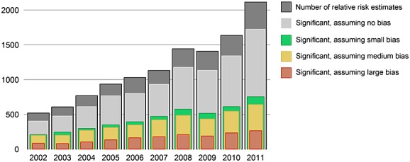
Effect estimates extracted from MEDLINE abstracts of observational studies using healthcare databases, by publication year. The number of estimates reaching statistical significance (p < 0.05) is estimated using four assumption on the null distribution: no bias (traditional significance testing): mean  =  0, SD  =  0; small bias: mean  =  0, SD  =  0.25; medium bias: mean  =  0.25, SD  =  0.25; large bias: mean  =  0.5, SD  =  0.5.

4. Discussion

Our reproduction of three observational studies published in literature produced similar odds and rate ratios, giving confidence that our studies are representative of real-world studies. Applying the same study design to sets of negative controls showed that all three studies were plagued by residual systematic error that had not been corrected for by the various study designs and data analyses. We do not believe that this problem is unique to our three studies, nor do we believe that these study designs are particularly bad designs. The papers from which the designs were borrowed represent excellent scientific studies, and Tata et al. ⁹ even went as far as including an SCCS in their analysis, a method that is believed to be less vulnerable to systematic error ⁶. We therefore must conclude that this problem is intrinsic to observational studies in general.

The notion of residual systematic error has already found some acceptance with methodologists, and several approaches for computing the potential impact of systematic error using a priori assumptions on potential source of error do exist (see ¹⁹ for an excellent review). However, very few observational studies have actually applied these techniques. Reasons for this include the need to make various subjective assumptions on the nature and magnitude of the systematic error, which themselves are subject to uncertainty, and the fact that some of these methods are highly complex. Using negative controls to empirically estimate the bias in a study provides a straightforward approach of interpreting the outcome of a study. The observed null distribution incorporates most forms of bias, including residual confounding, misclassification, and selection bias. The error distribution resulting from this bias (which does not depend on sample size) can be added to the random error distribution (which is based on sample size) to produce a single intuitive value: the calibrated p-value.

Our research is strongly related to previous research on estimating the false discovery rate (FDR) ^20–22, where an empirical null distributed is computed for either z-values or p-values ²². However, FDR methods were developed for analyzing high-throughput data representing many similar hypothesis tests. Most important, these tests typically have the same sample size and corresponding standard error. In the observational studies we investigated, we found widely differing standard errors even when using the same outcome, method, and database, primarily because of differences in drug prevalence. When applying FDR methods using z-value or p-value modeling, we found these methods had a counterintuitive property: large sample size (low standard error) could compensate for bias. For example, even when it was clear that a method was highly positively biased, we found highly prevalent drugs with effect estimates barely above one were still deemed statistically significant using these methods because of the large original z-value or small original p-value. Our intuition is that bias is irrespective of sample size and would remain present even in an infinitely large sample. We have therefore chosen to model our null distribution on the basis of the effect estimate, taking standard error into account as a measure of uncertainty.

We have demonstrated our approach in the field of drug safety but expect it could be applicable in other types of observational studies as well, as long as suitable negative controls can be defined. The most important characteristic of negative controls, apart from the fact that they are known not to cause the outcome, is that they somehow represent a sample of the bias that could be present for the exposure of interest. A completely random variable would make a poor negative control, because the bias will be zero, which is not what we would expect for any meaningful exposure of interest. For example, in nutritional epidemiology, other food types are most likely good negative controls, but the last digit of someone′s zip code is not.

One of the limitations of our study is the assumption that our negative controls truly represent drug–outcome pairs with no causal relationship. However, a few erroneously selected negative controls should not change the findings much, and we find it hard to believe that a large number of our negative controls are wrong. In FDR methods ²⁰ where there is no information on the presence of causal relationships, the majority of relationships ( > 90%) is simply assumed to be negative. Furthermore, we cannot say with certainty to what extent the results presented here are generalizable beyond the two databases (GE and Thomson MarketScan Medicare Supplemental Beneficiaries) used here. In no way would we suggest that the null distributions in other databases are comparable, even when using the same study design and analysis. For every database, the calibration process described here will have to be repeated. Another limitation is the notion that the same data, study design, and analysis can be used for different drugs. Although studies often already include more than one drug (for example, Tata et al. ⁹ studied both SSRIs and non-steroidal anti-inflammatory drugs), for some drugs, the study design would be deemed less appropriate because of known bias that would not be corrected for. For example, we identified some of our negative controls that might be confounded by indication, which might preclude the use of a case–control design. By removing those controls, we see only small changes in the fitted distribution. Furthermore, because we cannot pretend to know all bias that is present for the drug of interest, we would like to argue that we should include such negative controls to account for potential gaps in our knowledge.

For two of our three examples, we could not reject the null hypothesis of no effect after calibration, even though originally all three were considered highly statistically significant. The analysis of the effect estimates found in literature showed that the majority of significant results fail to reject the null hypothesis when even making the most modest assumptions of bias. This is in line with earlier estimations that most published research findings are wrong ⁵, although in this previous work, the main focus was on selective reporting bias (e.g., publication bias), which we have not even taken into consideration here. Reality may even be grimmer than our findings suggest, which is troubling because the evidence of these observational studies is widely used in medical decision making.

The method proposed here aims to correct the type I error (erroneously rejecting the null hypothesis) level, most likely at the cost of vastly increasing the number of type II errors (erroneously rejecting the alternative hypothesis). Ideally, we would improve our study designs to better control for bias, which would result in and approaching 0, and thereby maximizing statistical power after calibration. In that case, our approach would no longer be needed for calibration, only to show that bias has been dealt with. However, as shown here, the study designs currently pervading literature fall short of this goal, and more work is needed to reach this (potentially unobtainable) goal.

We recommend that observational studies always include negative controls to derive an empirical null distribution and use these to compute calibrated p-values.

Supporting Information

Supporting info item

References

- Mayes LC, Horwitz RI, Feinstein AR. A collection of 56 topics with contradictory results in case-control research. International Journal of Epidemiology. 1988;17:680–685. doi: 10.1093/ije/17.3.680. [DOI] [PubMed] [Google Scholar]
- Ioannidis JP, Tarone R, McLaughlin JK. The false-positive to false-negative ratio in epidemiologic studies. Epidemiology. 2011;22:450–456. doi: 10.1097/EDE.0b013e31821b506e. [DOI] [PubMed] [Google Scholar]
- Green J, Czanner G, Reeves G, Watson J, Wise L, Beral V. Oral bisphosphonates and risk of cancer of oesophagus, stomach, and colorectum: case-control analysis within a UK primary care cohort. BMJ. 2010;341:c4444. doi: 10.1136/bmj.c4444. [DOI] [PMC free article] [PubMed] [Google Scholar]
- Cardwell CR, Abnet CC, Cantwell MM, Murray LJ. Exposure to oral bisphosphonates and risk of esophageal cancer. Journal of the American Medical Association. 2010;304:657–663. doi: 10.1001/jama.2010.1098. [DOI] [PMC free article] [PubMed] [Google Scholar]
- Ioannidis JP. Why most published research findings are false. PLoS Medicine. 2005;2:e124. doi: 10.1371/journal.pmed.0020124. [DOI] [PMC free article] [PubMed] [Google Scholar]
- Farrington CP, Nash J, Miller E. Case series analysis of adverse reactions to vaccines: a comparative evaluation. American Journal of Epidemiology. 1996;143:1165–1173. doi: 10.1093/oxfordjournals.aje.a008695. [DOI] [PubMed] [Google Scholar]
- Rosenbaum P, Rubin D. The central role of the propensity score in observational studies for causal effects. Biometrika. 1983;70:41–55. [Google Scholar]
- Smith BM, Schwartzman K, Bartlett G, Menzies D. Adverse events associated with treatment of latent tuberculosis in the general population. Canadian Medical Association Journal. 2011;183:E173–179. doi: 10.1503/cmaj.091824. [DOI] [PMC free article] [PubMed] [Google Scholar]
- Tata LJ, Fortun PJ, Hubbard RB, Smeeth L, Hawkey CJ, Smith CJ, Whitaker HJ, Farrington CP, Card TR, West J. Does concurrent prescription of selective serotonin reuptake inhibitors and non-steroidal anti-inflammatory drugs substantially increase the risk of upper gastrointestinal bleeding. Alimentary Pharmacology & Therapeutics. 2005;22:175–181. doi: 10.1111/j.1365-2036.2005.02543.x. [DOI] [PubMed] [Google Scholar]
- McAfee AT, Ming EE, Seeger JD, Quinn SG, Ng EW, Danielson JD, Cutone JA, Fox JC, Walker AM. The comparative safety of rosuvastatin: a retrospective matched cohort study in over 48,000 initiators of statin therapy. Pharmacoepidemiology and Drug Safety. 2006;15:444–453. doi: 10.1002/pds.1281. [DOI] [PubMed] [Google Scholar]
- El-Serag HB, Everhart JE. Diabetes increases the risk of acute hepatic failure. Gastroenterology. 2002;122:1822–1828. doi: 10.1053/gast.2002.33650. [DOI] [PubMed] [Google Scholar]
- Jinjuvadia K, Kwan W, Fontana RJ. Searching for a needle in a haystack: use of ICD-9-CM codes in drug-induced liver injury. American Journal of Gastroenterology. 2007;102:2437–2443. doi: 10.1111/j.1572-0241.2007.01456.x. [DOI] [PubMed] [Google Scholar]
- Chan KA, Truman A, Gurwitz JH, Hurley JS, Martinson B, Platt R, Everhart JE, Moseley RH, Terrault N, Ackerson L, Selby JV. A cohort study of the incidence of serious acute liver injury in diabetic patients treated with hypoglycemic agents. Archives of Internal Medicine. 2003;163:728–734. doi: 10.1001/archinte.163.6.728. [DOI] [PubMed] [Google Scholar]
- Abraham NS, Cohen DC, Rivers B, Richardson P. Validation of administrative data used for the diagnosis of upper gastrointestinal events following nonsteroidal anti-inflammatory drug prescription. Alimentary Pharmacology & Therapeutics. 2006;24:299–306. doi: 10.1111/j.1365-2036.2006.02985.x. [DOI] [PubMed] [Google Scholar]
- Cooper GS, Chak A, Lloyd LE, Yurchick PJ, Harper DL, Rosenthal GE. The accuracy of diagnosis and procedural codes for patients with upper GI hemorrhage. Gastrointestinal Endoscopy. 2000;51:423–426. doi: 10.1016/s0016-5107(00)70442-1. [DOI] [PubMed] [Google Scholar]
- Andrade SE, Gurwitz JH, Chan KA, Donahue JG, Beck A, Boles M, Buist DS, Goodman M, LaCroix AZ, Levin TR, Platt R. Validation of diagnoses of peptic ulcers and bleeding from administrative databases: a multi-health maintenance organization study. Journal of Clinical Epidemiology. 2002;55:310–313. doi: 10.1016/s0895-4356(01)00480-2. [DOI] [PubMed] [Google Scholar]
- Lipsitch M, Tchetgen Tchetgen E, Cohen T. Negative controls: a tool for detecting confounding and bias in observational studies. Epidemiology. 2010;21:383–388. doi: 10.1097/EDE.0b013e3181d61eeb. [DOI] [PMC free article] [PubMed] [Google Scholar]
- Tisdale JE, Miller DA. Drug-Induced Diseases. Prevention, Detection, and Management, Bethesda, MD: American Society of Health-System Pharmacists; 2010. [Google Scholar]
- Gustafson P, McCandless LC. Probabilistic approaches to better quantifying the results of epidemiologic studies. International Journal of Environmental Research and Public Health. 2010;7:1520–1539. doi: 10.3390/ijerph7041520. [DOI] [PMC free article] [PubMed] [Google Scholar]
- Efron B. Large-scale simultaneous hypothesis testing: the choice of a null hypothesis. Journal of the American Statistical Association. 2004;99:96–104. [Google Scholar]
- Langaas M, Lindqvist BH, Ferkingstad E. Estimating the proportion of true null hypotheses, with application to DNA microarray data. Journal of the Royal Statistical Society Series B. 2005;67:555–572. [Google Scholar]
- Strimmer K. A unified approach to false discovery rate estimation. BMC Bioinformatics. 2008;9:303. doi: 10.1186/1471-2105-9-303. [DOI] [PMC free article] [PubMed] [Google Scholar]
Associated Data
This section collects any data citations, data availability statements, or supplementary materials included in this article.
Supplementary Materials