GraSP: Geodesic Graph-based Segmentation With Shape Priors for the Functional Parcellation of the Cortex

Abstract

Resting-state functional MRI is a powerful technique for mapping the functional organization of the human brain. However, for many types of connectivity analysis, high-resolution voxelwise analyses are computationally infeasible and dimensionality reduction is typically used to limit the number of network nodes. Most commonly, network nodes are defined using standard anatomic atlases that do not align well with functional neuroanatomy or regions of interest covering a small portion of the cortex. Data-driven parcellation methods seek to overcome such limitations, but existing approaches are highly dependent on initialization procedures and produce spatially fragmented parcels or overly isotropic parcels that are unlikely to be biologically grounded.

In this paper, we propose a novel graph-based parcellation method that relies on a discrete Markov Random Field framework. The spatial connectedness of the parcels is explicitly enforced by shape priors. The shape of the parcels is adapted to underlying data through the use of functional geodesic distances. Our method is initialization-free and rapidly segments the cortex in a single optimization. The performance of the method was assessed using a large developmental cohort of more than 850 subjects. Compared to two prevalent parcellation methods, our approach provides superior reproducibility for a similar data fit. Furthermore, compared to other methods, it avoids incoherent parcels. Finally, the method’s utility is demonstrated through its ability to detect strong brain developmental effects that are only weakly observed using other methods.

1. Introduction

Resting-state fMRI (rsfMRI) has emerged as a valuable tool for understanding the functional organization of the brain in both health (Yeo et al., 2011; Power et al., 2011) and disease (Leistedt et al., 2009; Baker et al., 2014; Lynall et al., 2010; Varoquaux et al., 2010). It has been widely adopted as a tool for understanding functional connectivity in the brain. The high dimensionality of these spatio-temporal images, however, is an impediment for extracting stable, reproducible and interpretable functional networks from rsfMRI data, necessitating effective dimensionality reduction methods. According to the segregation and integration principles (Tononi et al., 1994), information is processed in the brain by compact groups of neurons that collaborate as functional units. Rationally grouping neighboring brain regions that have similar activity patterns provides efficient dimensionality reduction for connectivity studies that focus on the interaction among these units. In this paper, we focus on methods producing a regional parcellation (Craddock et al., 2012), unlike ICA based methods (Calhoun et al., 2001; Smith et al., 2012) and sparse dictionary based methods (Varoquaux et al., 2011) that segment functional networks. These functional parcellations can provide a reduced set of functional units, to be further used in conjunction with ICA (Calhoun et al., 2001; Smith et al., 2012), graphical theoretical analysis (Bullmore and Sporns, 2009) or sparse network reconstruction methods (Eavani et al., 2013).

Data-driven parcellation methods proposed so far can be grouped into three broad categories.

The first category includes methods originating from the data mining literature. They cluster the different locations of the brain according to the similarity between their activation time-series (Shen et al., 2013; Cordes et al., 2002; Lashkari et al., 2010b; Blumensath et al., 2013; Honnorat et al., 2013). In these approaches, the geometry of the cortex is taken into account via the introduction of additional constraints, in particular when connected parcels are sought. Such grouping has been performed using K-means (Bellec et al., 2010; Mezer et al., 2009), fuzzy clustering (Baumgartner et al., 1997), spectral clustering (Thirion et al., 2006; van den Heuvel et al., 2008; Craddock et al., 2012; Shen et al., 2010, 2013; Kim et al., 2010; Yeo et al., 2011), affinity propagation (Frey and Dueck, 2007; Zhang et al., 2011) and hierarchical clustering (Salvador et al., 2005; Cordes et al., 2002). A hierarchical clustering parcellation is also the starting point of the method proposed in (Michel et al., 2012) that derives discriminative brain partitions in a supervised fashion. Critically, all of the existing approaches suffer from certain limitations: they require and are sensitive to initialization parameters (K-means clustering), rely on a heuristic (hierarchical clustering) or are known to provide overly isotropic parcels (spectral clustering; Craddock et al., 2012).

The second family of methods encompass numerous continuous graphical models, that model the generation of the rs-fMRI data observed. In the past, fMRI data has been modeled as a mixture of Gaussian components in (Golland et al., 2007; Tucholka et al., 2008), a mixture of von MisesFisher distributions (Lashkari et al., 2010b) or a mixture of Dirichlet processes (Jbabdi et al., 2009); continuous Markov Random Fields were proposed in (Liu et al., 2011, 2012). In the recent years, parcellation has been performed by models of increasing complexity accounting for variable number of parcels, multiple subjects comparison and spatial smoothness (Lashkari and Golland, 2009; Lashkari et al., 2010a). In these models, the optimization is jointly performed on the parcel labels and model parameters, through variational EM (Dempster et al., 1977) or Gibbs sampling. The recent approaches optimize a large number of parameters and rely on iterative or approximated solvers, which may impact the quality of the local optimum obtained.

The third family of methods originates from the computer vision literature. They require a graph encoding the geometry of the cortex, which is then segmented into compact components (Blumensath et al., 2013). Region growing is a common approach (Bellec et al., 2006; Heller et al., 2006; Lu et al., 2003; Blumensath et al., 2012, 2013). However, region growing requires initial seed regions, which are gradually enlarged and fused.

Generally, all of the above approaches are strongly initialization dependent or rely on complex models. As a result, their reproducibility is limited (Blumensath et al., 2013). Since the parcellation of a graph is a hard problem, unless P=NP, no method will perfectly address all these concerns. However, restricting the complexity of the approach, removing the initialization step (which could guide the method toward bad local optima) and exploiting advanced solvers could provide a substantial advance over existing methods and improve reproducibility. Therefore, we present a discrete MRF based segmentation approach. We propose a method that strongly imposes connectedness on the parcels, contrary to most continuous graphical models. Our data modeling is simpler than recent advanced continuous models (Lashkari and Golland, 2009; Lashkari et al., 2010a) but this simplicity portends a higher robustness, as our method does not rely on the estimation of numerous parameters. The discrete model proposed here is optimized by specific efficient solvers derived from graph theory (Boykov et al., 2001). Contrary to region growing and many clustering based methods, our method does not require an initialization.

This approach was suggested in part by previous work using MRF (Ryali et al., 2013), which we built upon a connectedness constraint in preliminary studies (Honnorat et al., 2013). Contrary to the original method of Ryali et al. that was used for segmenting small brain regions (Ryali et al., 2013), our method can segment the entire cortex into properly connected regions.

Here, we validated our approach on a large neurodevelopment data-set (Satterthwaite et al., 2014). Results demonstrate the superior performance of our method compared to two common parcellation approaches. As described below, we found that our constrained MRF method rapidly segments the human cortex with improved reproducibility compared to other methods. Finally, an application to neurodevelopment reveals robust developmental effects of interest, to which other methods are less sensitive.

2. Materials and Methods

Markov Random Fields (MRF) constitute a mature and versatile tool that has been useful for many computer vision and imaging tasks, such as registration (Glocker et al., 2011) and segmentation (Wang and Komodakis, 2013). For rs-fMRI processing, MRF were used for signal denoising (Descombes et al., 1998) and segmentation (Lashkari et al., 2010b; Liu et al., 2010, 2012, 2011). Most of the graph-based segmentation schemes proposed so far rely on continuous models, that are optimized by Gibbs sampling (Lashkari et al., 2010b; Liu et al., 2010) or variational methods (Lashkari and Golland, 2009).

By contrast, we propose a discrete formulation. Similar to the approach in (Ryali et al., 2013), the segmentation is performed by an efficient solver relying on graph cuts (Boykov et al., 2001; Komodakis and Tziritas, 2007; Komodakis et al., 2008). Contrary to (Ryali et al., 2013), however, our model segments the brain into parcels that are guaranteed to be spatially connected: the fragmentation of brain regions into discontinuous parts is prevented, which allows us to control the number of parcels precisely.

Connectedness is a challenging property to achieve with MRF segmentation scheme, because they rely on local interactions, while connectedness is a global property that can not be enforced locally. For this reason, this property was not modeled by other discrete graphical models before our preliminary work (Honnorat et al., 2013). In our approach, connectedness is guaranteed by enforcing a stronger topological property using shape priors. Shape priors (Veksler, 2008; Gulshan et al., 2010) are used for enforcing the star convexity of the parcels. By definition, this property states that there exists a node in each parcel that is connected to all the nodes of the parcel by at least one geodesic path entirely included in the parcel. This property implies that for all the parcels, any pair of nodes can be linked by a path that is entirely within the parcel. This is the topological definition of connectedness.

The current paper builds upon preliminary work presented in (Honnorat et al., 2013), by extending it in several ways. First, a reformulation rendered initialization completely unnecessary. Second, the cortex is parcellated in only one optimization step, using a different solver. This approach is simultaneously easier to implement, faster and more robust because the dependency on the initialization was removed. We finally present a comparison of our discrete MRF approach with alternative methods on a large database (≈ 850 scans) including detailed reproducibility experiments and novel scores accounting for the quality of the parcellations.

2.1. Graph-based Parcellation Model

This work adopts the traditional functional preprocessing procedure (Blumensath et al., 2013; Ryali et al., 2013). A mesh capturing the geometry of the cortex is first extracted using Freesurfer (Dale et al., 1999) and the rs-fMRI signal is projected on that mesh. A graph parcellation method is then applied, with the aim of clustering neighboring cortical locations into geometrically compact parcels according to a measure of the similarity of the time-series.

Several similarity measures were proposed for comparing the time-series of cortical regions. Simulation studies have shown that “full” correlation and partial correlation measures are reliable for network identification (Smith et al., 2011). Hence, in this paper, we adopt full correlations as the similarity measure between cortical node time-series and the related Pearson distance (Blumensath et al., 2013; Ryali et al., 2013; Honnorat et al., 2013). However, any similarity criterion and associated distance could be utilized within our modular framework.

Let us assume that a mesh 𝒫 of N cortical nodes has been extracted. We assume that the average signal of each parcel is represented by the signal of one of its nodes, which lies near the geometric center of the parcel. This node is referred to the parcel center in the remainder of the paper. The purpose of the parcellation is to determine a label l_j for each mesh node j that indicates which parcel should contain j. Since a parcel center belongs to only one parcel, we identify the parcels with their center: a parcel center is a node such that l_i = i and for any i ∈ 𝒫, the parcel i is the set of nodes j with labels l_j = i.

Our parcellation framework, GraSP, consists of three parts. (i) The functional coherence of the parcels is enforced by singleton potentials V_i(l_i), that diminish when the node i is assigned to a parcel l_i that is well correlated with its signal. (ii) The number of parcels is penalized by a sum of label costs L_i({l_j}_j∈𝒫), that penalize the introduction of a parcel of center i. (iii) The connectedness of the parcels is enforced using a star shape prior W_i({l_j}_j∈𝒫) for each parcel i. As a result, the optimal parcellation is determined by minimizing the following energy:

$$E({\{l_i\}}_{i\in 𝒫})=\sum _{i\in 𝒫}{V}_i(l_i)+L_i({\{l_j\}}_{j\in 𝒫})+W_i({\{l_j\}}_{j\in 𝒫})$$

The first two components of the model are described in the following section. They model the segmentation of the rs-fMRI data into a small number of functionally coherent parcels and is similar to the method proposed in (Ryali et al., 2013). One of the specific contributions of this paper, the functional shape priors W_i, is presented in the next section. These potentials prevent the fragmentation of the parcels into small regions as in (Ryali et al., 2013), allowing to precisely penalize the number of connected components, for any size of the cortical mesh.

2.2. Resting-state Data Modeling

Correlations and partial correlation are often used for measuring the similarity between activation time-series (Craddock et al., 2012; Blumensath et al., 2013; Lashkari et al., 2010b) and their robustness was validated on synthetic data (Smith et al., 2011). Our signal model tends to assign the nodes of the mesh to the parcels with the most similar signal, while penalizing the number of parcels. This behavior is dictated by two families of potentials: i) singleton “data potentials” favoring high correlation between a node and the signal of the parcel it is assigned to, and ii) labels costs penalizing the number of parcels.

Let us describe with i ∈ 𝒫 one of the node of the cortical mesh 𝒫 and with y_i the time-series of i. For the sake of simplicity, we will now only deal with normalized de-meaned time-series:

$${\mathbf{z}}_i=\frac{{\mathbf{y}}_i-y(i)}{{\Vert {\mathbf{y}}_i-y(i)\Vert }_2^2}$$

Where y(i) is the average of the BOLD signal y_i of the node i. With the above notation, the data singleton potentials introduced for each mesh mode, V_i(l_i), is given by:

$$V_i(l_i)=-\langle {\mathbf{z}}_i,{\mathbf{z}}_{l_i}\rangle$$

where 〈,〉 denotes the standard inner product.

The label costs penalize the presence of a given label in a segmentation result (Delong et al., 2012). For each parcel i, the following cost is introduced:

$$L_i({\{l_j\}}_{j\in 𝒫})=\{\begin{array}{cc}K\hfill & \exists j|l_j=i\hfill \\ 0\hfill & \text{otherwise}\hfill \end{array}$$

This potential adds a cost K as soon as a node j is assigned to the parcel i. Label costs are high-order MRF potentials, which can be decomposed into a sum of singleton and sub-modular pairwise potentials by introducing supplementary variables (Kohli and Kumar, 2010). Delong et al. suggested a new approach, that efficiently manages the labels costs by modifying a well-known MRF solver (Delong et al., 2012). Contrary to our preliminary work (Honnorat et al., 2013), the second approach was adopted here, and a similar label cost of value K was introduced for all the parcels. Since our singleton cost is fixed, K is also the parameter that balances the high-order potentials with respect to the singleton costs. As opposed to the model (Ryali et al., 2013), we have removed the spatial smoothing term for the sake of simplicity and with the aim of obtaining irregular parcels, as suggested by (Blumensath et al., 2013).

So far, the potentials that we have introduced are based only on the fMRI signal. Because connectedness is a geometric/topologic property, it requires a new set of potentials that are described in the next section.

2.3. Connectedness Enforcement

Connectedness is very challenging to achieve with MRF, because this is a global property that takes the whole segmentation into account, while graphical models are based on local interactions. We impose a stronger property that guarantees connectedness and is easier to model in discrete MRF: star-convexity. A set is star convex with respect to a center when the shortest path between any point of the set and the center is included in the set. It was proved that star convexity can be enforced in a MRF framework by introducing simple, sub-modular, pairwise potentials (Veksler, 2008). Below, we will refer to the sum of these potentials as “star shape prior”. Gulshan et al. suggested considering a geodesic data-dependent distance when deriving the shortest paths, in order to adapt the shape prior and have access to a broader set of parcel shapes (Gulshan et al., 2010). We propose to enforce the connectedness of the parcels with geodesic star shape priors based on the Pearson distance between the neighboring nodes of the cortical mesh. Their ability to fit challenging shapes is illustrated in section 4.2.2.

The geodesic star shape priors are built in the following manner. First, the Pearson distance between each pair of neighboring nodes i,j of the cortical mesh 𝒫 is computed:

$$d(i,j)=1-\langle {\mathbf{z}}_i,{\mathbf{z}}_j\rangle$$

The shortest paths through the mesh are computed in order to extend the definition of d to all the pairs of nodes. The figure (1) presents one of the geodesic distance map obtained.

Figure 1.

(a) For one of the subjects of the database: geodesic distances from a mesh node located in the cuneus (black cross), visualized on the inflated brain surface and on the pial brain surface. The irregularity of the distance level sets illustrates the ability of our geodesic distance to produce anisotropic parcel shape priors. (b) illustration of the constraints introduced by a shape prior. The black node i is the candidate parcel center. When a node j of the mesh is assigned to this center, the shape prior forces the neighboring node of j that is the closest to the center i according to the geodesic distance map, 𝒩(j,i) to be assigned to the center as well.

Once the geodesic distances have been computed, the shape priors are defined in the following manner: the connectedness of each parcel (of center) i is enforced by a shape prior W_i({l_j}_j∈𝒫) equal to the sum of pairwise potentials:

$$W_i({\{l_j\}}_{j\in 𝒫})=\sum _{j\in 𝒫}{W}_{i,j,𝒩(j,i)}(l_j,l_{𝒩(j,i)})W_{i,j,k}(l_j,l_k)=\{\begin{array}{cc}\infty \hfill & l_j-i\text{and}{l}_k\ne i\hfill \\ 0\hfill & \text{otherwise}\hfill \end{array}$$

where 𝒩(j,i) is the neighbor of the node j that is the closest to i, according to our geodesic distance d. Thus, when a node j is assigned to the parcel of center i, the node 𝒩(j,i) is constrained to be part of the parcel. Because 𝒩(j,i) is the closest point to j belonging to the shortest geodesic path between j and i, from node to node, these constraints guarantee that the whole shortest geodesic path between j and i is part of the parcel. This ensures the star-convexity of the parcel with respect to its center i. The construction of a star shape potential is shown in figure (1). In practice, the maximum value of W_i,j,k (theoretically infinite) was set to a value much larger than K and the singleton potentials (that are all lower than 2), in order to ensure that the shape priors dominate all the other terms and act like hard constraints.

In our framework, particular attention was paid to introducing only sub-modular potentials. For this reason, the optimization of our parcellation model can be solved by efficient solvers (Boykov et al., 2001; Delong et al., 2012) that optimize the MRF energy by performing a sequence of fast label expansions using a graph-cut algorithm.

The next section describes the indices that we have measured for assessing the performance of GraSP and the other parcellation methods that were tested on our data and provides further implementation details.

3. Validation Measures and Comparison with Existing Methods

This section presents the measures that were employed for comparing the parcellations across subjects, the different parcellation methods that we have tested, and how they were compared. Two indices measuring the reproducibility of the parcellation are first presented. The fit of the parcellation to the rs-fMRI signal is also evaluated using a set of measures that is presented in the second section. The third section presents the clustering approaches that we have compared with our method. Implementation details conclude the section.

3.1. Dice and Adjusted Rand Indices

In our framework, two parcellations do not necessarily contain the same number of parcels. Also, the parcels indices do not reflect their spatial proximity. For these reasons, the metrics that are classically employed in the registration literature are impractical, unless the parcels are matched across the parcellations (Blumensath et al., 2013). Such an approach requires a matching algorithm, which is time consuming and suffers from approximation when a one-to-one matching is performed (since such settings cannot match all the parcels). Because one-to-one matches are the only ones that can be performed efficiently, e.g. using the Hungarian method (Lange et al., 2004) and other strategies involve NP hard problems, this approach necessarily leads to complicated and unsatisfying comparisons.

We address this concern by exploiting clustering comparison metrics. Many such metrics deal with varying num-bers of clusters/parcels, and a review (Pfitzner et al., 2009) compares more than fifty similarity metrics that meet our requirements.

We have chosen two standard measures: the adjusted Rand index (aR) and the Dice index generalized for the simultaneous comparison of multiple clusters (Di). These were introduced in (Hubert and Arabie, 1985) and (Dice, 1945) respectively. These indices are efficiently computed from the elements of the mismatch matrix between the clusterings/parcellations. Let us denote with X = {x} and Y = {y} two parcellations (x and y are parcels) of the whole cortex and |x| the number of cortical nodes assigned to the parcel x. The mismatch matrix (m_x,y) contains one element m_x,y for each parcel x of the first parcellation and each parcel y of the second one, that is equal to the number of nodes that are shared by these two parcels:

$$m_{x,y}=|x\cap y|$$

The indices are computed from m_x,y and the sums a_x = Σ_y m_x,y and b_y = Σ_x m_x,y in the following manner:

$$Di=\frac{2a}{2a+b+c}aR=\frac{{\mathrm{\Sigma }}_{x,y}\left(\begin{array}{c}\hfill m_{x,y}\hfill \\ \hfill 2\hfill \end{array}\right)-\left[{\mathrm{\Sigma }}_x\right(\begin{array}{c}\hfill a_x\hfill \\ \hfill 2\hfill \end{array}\left){\mathrm{\Sigma }}_y\right(\begin{array}{c}\hfill b_y\hfill \\ \hfill 2\hfill \end{array}\left)\right]/\left(\begin{array}{c}\hfill N\hfill \\ \hfill 2\hfill \end{array}\right)}{\frac{1}{2}\left[{\mathrm{\Sigma }}_x\right(\begin{array}{c}\hfill a_x\hfill \\ \hfill 2\hfill \end{array})+{\mathrm{\Sigma }}_y(\begin{array}{c}\hfill b_y\hfill \\ \hfill 2\hfill \end{array}\left)\right]-\left[{\mathrm{\Sigma }}_x\right(\begin{array}{c}\hfill a_x\hfill \\ \hfill 2\hfill \end{array}\left){\mathrm{\Sigma }}_y\right(\begin{array}{c}\hfill b_y\hfill \\ \hfill 2\hfill \end{array}\left)\right]/\left(\begin{array}{c}\hfill N\hfill \\ \hfill 2\hfill \end{array}\right)}$$

where N is the size of the cortical mesh and a,b and c are defined as follows:

$$a=\frac{1}{2}\sum _{x,y}{m}_{x,y}(m_{x,y}-1)b=\frac{1}{2}[\sum _x{a}_x^2-\sum _{x,y}{m}_{x,y}^2]c=\frac{1}{2}[\sum _y{b}_y^2-\sum _{x,y}{m}_{x,y}^2]$$

The Dice and adjusted Rand indices assess the reproducibility of the parcellation, but a high reproducibility does not necessarily relate to good segmentation performance. The fit of the parcellation to the rs-fMRI data needs to be estimated as well when comparing parcellation methods, as some methods could have high reproducibility but fit the data poorly. The next section presents the measures that were adopted for this purpose.

3.2. Functional Coherence Measures

In order to measure the functional homogeneity of the parcellation, we introduced two indices. The first is a global index that was measured in the following manner. Let denote with X a parcellation segmenting the cortical mesh 𝒫 into n parcels x_i, i = 1 …n. The average signal z(x_i) of each parcel x_i was computed. Then, the correlation ratio between all the nodes of the parcels and the average signal was computed. Fisher z-transform:

$$f(r)=\frac{1}{2}ln\left(\frac{1+r}{1-r}\right)$$

was applied to these correlation ratios in order to obtain real scores that can be averaged. The average of the scores over the whole cortical mesh was used for measuring the functional homogeneity of the parcels. We refer to this as the Average Functional Coherence (AFC). The AFC increases when the signals of the nodes of the parcels are better correlated, and summarizes the global quality of a parcellation. However, it suffers from two limitations. First, it takes only the parcel coherence into account. As a result, it necessarily improves when the size of the parcels is reduced. Second, it computes a global fit to the data that does not take into account the quality of the individual parcels, and does not penalize methods that produce incoherent parcels.

In order to address these concerns, a variant of Dunn index (Dunn, 1973) was also adopted, that will be denoted as Functional Clustering Index (FCI). The FCI of a parcellation is equal to the ratio between the smallest Pearson distance between the averaged signals z(x_i) of the parcels x_i and the maximal functional heterogeneity of a parcel:

$$FCI(X)=\frac{{\text{min}}_{i,j}\{1-\langle \mathbf{z}(x_i),\mathbf{z}(x_j)\rangle \}}{{\text{max}}_i\mathrm{\Delta }(x_i)}$$

The Pearson distance associated with the “average” correlation inside the parcel was calculated for measuring the functional heterogeneity of a parcel, which is denoted as parcel scatter:

$$\mathrm{\Delta }(x_i)=1-f^{-1}(\frac{1}{|x_i|}\sum _{p\in x_i}f(\langle {\mathbf{z}}_p,\mathbf{z}(x_i)\rangle ))$$

where the inverse of the Fisher z-transform is given by:

$$f^{-1}(r)=\frac{e^{2r}-1}{e^{2r}+1}$$

The FCI increases when the parcels are more coherent and when the distance between the parcels signal increases. We increased the robustness of the index by replacing the minimum and the maximum with quantiles. Because the number of inter-parcel distances is proportional to the square of the number of parcels, we considered a tighter approximation for the numerator. More precisely, FCI_10%(X) will denote the FCI measured when the maximum parcel scatter is replaced by the ninth decile of the parcel scatter and the minimum of the inter-parcel distance is replaced by the smallest centile of the inter-parcel distances. It is strongly related to the indices that were proposed in the data mining literature for estimating the number of parcels from the data: the Dunn (Dunn, 1973) and Davies-Bouldin (Davies, 1979) indices as well as the Silhouette index that is also often used for the same purpose (Rousseeuw, 1987).

During our experiments, both AFC and FCI were measured; for our method and the alternate methods presented in the next section.

3.3. Comparison with Existing Methods

We compare the parcellation method presented in this paper, GraSP, with two clustering methods. The Ward hierarchical clustering method (Ward, 1963) was considered first. This agglomerative hierarchical clustering algorithm starts with singleton parcels, and iteratively merges neighboring parcels until the requested number of clusters is reached, in such a way that the variance of the parcels remains low. Such an approach has already been considered for segmenting fMRI data (Cordes et al., 2002; Salvador et al., 2005; Michel et al., 2012; Blumensath et al., 2013). For our experiments, we considered the normalized signals z_p and processed them with the Scikit-learn implementation of Ward clustering (Pedregosa et al., 2011).

A spectral clustering method was also considered (Shi and Malik, 2000). This algorithm first builds a dissimilarity matrix that is used for finding a projection of the data in a space where they are easier to cluster. A K-means clustering is finally performed in that space. As suggested by Shen et al. (Shen et al., 2010), we reduced the size of the similarity matrix by considering only the Pearson distances between the time-series of neighboring nodes. For each node, we considered approximately 400 neighbors (≈ 4% of the full graph) that were chosen according to their distance to the node (lower than 10 edges). The same weight matrix was computed and scaled by the median of the functional distance (Shen et al., 2010). Each K-mean clustering was repeated 10 times.

In order to obtain comparable results, these algorithms were run after our method while controlling for the same number of clusters. The next section describes the implementation improvements that were introduced to significantly increase the speed of our method during our experiments.

3.4. Implementation Details

In order to determine the pairs of cortical nodes that are constrained by the star-shape priors, it is necessary to compute the geodesic distances between all the pairs of nodes. The Floyd-Warshall algorithm could perform this task, but we used a Dijkstra’s algorithm variant known to perform faster on sparse graphs: the Johnson’s algorithm (Johnson, 1977). Contrary to our preliminary work (Honnorat et al., 2013), we used the MRF optimizer (Boykov et al., 2001; Kolmogorov and Zabih, 2004; Boykov and Kolmogorov, 2004; Delong et al., 2012). This choice was dictated by the different time/memory trade-off offered, which is more favorable when the MRF involves many different labels (in our case: more than 10k). The computational time was significantly reduced by restricting the span of the shape priors to a value ρ. A node j was only considered in a star shape prior of center i when its geodesic distance to i, d(i, j) was smaller than ρ. We set this maximum parcel radius to ρ = 10d_average, where d_average is the average Pearson distance between neighboring nodes of the cortical mesh. This operation discarded a large number of useless potentials and allowed us to fully exploit the acceleration abilities of the solver (Delong et al., 2012). The computational time was considerably reduced, and our implementation reached the speed of the other algorithms. For all the methods tested, the computational time was lower than ten minutes per parcellation on a standard office computer. The next section presents the parcellation results obtained at different resolutions/number for parcels and for the different age groups.

4. Results

To test our method, we used a sample of 859 subjects from the Philadelphia Neurodevelopmental Cohort (Satterthwaite et al., 2014). The next section highlight the limitations of the model introduced in (Ryali et al., 2013) and illustrates the flexibility of the geodesic star shape priors that we have chosen. The parcellation results are presented in the next section. The following section presents a detailed comparison of the three methods according to the measures presented in the previous section: Dice and adjusted Rand index, average functional coherence (AFC) and functional clustering index (FCI). The next section investigates age related trends and the ability of the different methods to highlight these trends. An identification of the default mode network in the group parcellations concludes this experimental section. This validation illustrates also the future exploitation of our method.

4.1. Databases and Preprocessing

We validated our method using 859 rs-fMRI scans. For each subject, a T1 image was acquired prior to a 6 minutes long fMRI scan at TR of 3000 ms (120 time-points). Each fMRI scans was first registered to its related T1 using (Greve and Fischl, 2009) with distortion correction provided by FSL 5 (Jenkinson et al., 2012). The T1 images were registered to the FreeSurfers fsaverage5 cortical template (10,242 nodes/hemisphere) (Dale et al., 1999). The fMRI subjects timeseries was projected to the fsaverage surface space using FreeSurfers mrivol2surf command. Motion correction was performed through confound regression (Satterthwaite et al., 2013). The rs-fMRI time-series were finally band-pass filtered in order to retain only the signal between 0.01 and 0.08 Hz.

As the left and right hemispheres are segmented separately by FreeSurfer, all the parcellation results presented were produced for the two hemispheres separately and are presented accordingly. The subjects were divided into three age groups: 8–14 years old (249 scans), 14–18 years old (357 scans) and 18–24 years old (253 scans). In order to reduce the effect of inter subject variability, the methods were compared in a group parcellation setting. The reproducibility of the parcellation methods was assessed by randomly dividing each group into 5 disjoint sets of scans, that were concatenated and parcellated. The reproducibility was measured by computing the Dice and Rand indices between all the pairs of parcellations, which provided $\left(\begin{array}{c}5\hfill \\ 2\hfill \end{array}\right)=10$ values for each age group and each cortical hemisphere.

4.2. Shape Priors Utility and Flexibility

4.2.1. Parcels Fragmentation

In this section, we show that even a significant parcellation smoothing can not prevent the method of (Ryali et al., 2013) from generating segments made of multiple parts. For this reason, the parcel cost does not grant the user a direct control of the number of parcels, unless a significant smoothing is applied, which results in isotropic parcels.

This validation was carried out using all the scans of the oldest subject groups (5 concatenated rs-fMRI scans, for each hemisphere). A non iterative version of (Ryali et al., 2013) corresponding to the following model was implemented:

$$E({\{l_i\}}_{i\in 𝒬})=\sum _{i\in 𝒬}{V}_i(l_i)+\sum _{i\in 𝒬}{L}_i({\{l_j\}}_{j\in 𝒫})+\nu \sum _{i,j\in 𝒩(i)}P(l_i,l_j)$$

Where the singleton costs V_i and labels costs L_i were described in sections 2.1 and 2.2, 𝒩(i) is the set of neighbors of the node i, P(l_i, l_j) is the classical Potts potential and the set of admissible labels 𝒬 contains 1000 mesh nodes randomly selected. The smoothing of the segmentation is controlled by the parameter ν: high ν leads to fewer, isotropic parcels, because the Potts potential penalize the length of the frontier between the segments.

This energy was optimized in one step using the solver (Delong et al., 2012). The figure 2.a reports the number of labels and the number of connected components obtained for ten different values of the labels cost K = {1,2,…10} and three different amounts of regularization ν = {0.05,0.1,0.15}. The regularization of the segmentation prevents the apparition of isolated nodes and small fragments. However, many segments are divided into large fragments, such as the red fragments (highlighted with black arrows) in the figure 2.b that correspond to the default mode network.

Figure 2.

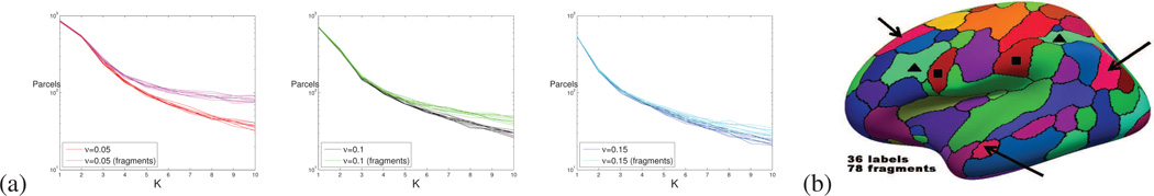
(a) Number of labels/segments introduced by the variant of (Ryali et al., 2013) tested, and true number of connected components (fragments) obtained. (b) One of the segmentation for ν = 0.05, where three fragmented segments have been highlighted (respectively with black squares, black triangles and black arrows).

When the parcel cost increases, the number of labels and the number of connected fragments diverge, as the algorithm starts merging nodes from different parts of the brain. An increased regularization of the segmentation delays this phenomenon, but generates isotropic parcels that are less realistic. Without smoothing, we obtained very fragmented results. Our dataset seems to be not very well adapted for investigating unconstrained clustering algorithms like (Thirion et al., 2014), unless very large parcels are required.

By contrast, shape priors have the advantage of preventing the fragmentation without smoothing the parcellation. In the next section, we demonstrate on a synthetic image that the geodesic shape prior based on Pearson distances that we have chosen is flexible enough to segment complex shapes.

4.2.2. Advantages of the Geodesic Shape Priors

Following (Gulshan et al., 2010), we parcellated a complex shape made of several loops in a 2D image. Each pixel of the image was considered as a node, and each node was linked to its 4 closest neighbors. The node timeseries considered were the RGB values at each pixel. Our parcellation algorithm was applied with parameters (K,ρ) = (10,0.05). Figure 3 presents the original image and its parcellation. The main parcel, containing the letter, is depicted in white (and its center is marked in red). In figure 4, we compare the supports of the smallest Euclidean and geodesic shape priors centered like the main parcel and containing all the pixels of the letter. These supports contain all the pixels that would belong to the main parcel if all the pixels of the letter were included. The geodesic shape prior and the underlying geodesic distance map clearly fit the data. They are perfectly able to handle tortuous parcels with holes, contrary to the Euclidean shape priors (Veksler, 2008). Such parcels being much more complex than the cortical functional areas, we think that the geodesic priors that we have chosen are flexible enough to not overconstrain the parcellation.

Figure 3.

(a) Original image (japanese hiragana character YU with yellow gausssian noise) (b) Parcellation: except the main parcel (in white), all the parcels are depicted with different green colors. The center of the main parcel is marked in red.

Figure 4.

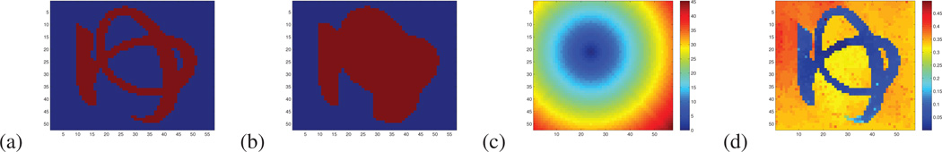
(a) Support of the smallest shape prior related to the main parcel containing all the pixel of the letter. (b) Support of the smallest Euclidean shape prior centered at the same location containing all the pixel of the letter. (c) Euclidean distance map from the center of the shape prior. (d) Pearson geodesic distance map.

4.3. Parcellation Results

In this section, we first present parcellations generated by our algorithm for different parcel costs/resolutions. The reproducibility results are then provided. We conclude the section by reporting the parcellation fit to the data, and the functional clustering indices obtained with the different methods.

All the experiments were reproduced four times, with the following parcel cost values: K = (75,15,10,5) and ρ = 10.0, more parcels being introduced as the parcel cost declines. With such parameters, the segmentations contain between 50 and 200 parcels, which corresponds to the number of nodes classically handled during connectivity analyses (Power et al., 2011). When less than 200 parcels are considered, they contain also more than 50 nodes in average (the fsaverage5 graph containing 10,242 nodes), which guarantees that the statistical analyses carried out at the parcel level are valid (normality can be assumed). Figure 5 presents the parcellations obtained for one concatenated group of fMRI scans. The number of parcels is reported in figure 6, for all the experiments. We present also in this figure a complete analysis of the variation of the number of parcels with the parameters K and ρ: the 10 concatenated scans of the oldest group of subjects where parcellated for all the parcels costs K = 2,4,…50 and five parcel maximal geodesic radii ρ = (5.0,7.5,10.0,15.0,20.0) (total: 1250 parcellations). When ρ is large, the parcels reach the maximum size at a larger K (but the computational burden is increased as well). While K is small enough with respect to the maximal radius, the curves of a same scan describe the same (purely data driven) relationship between K and the number of parcels (ρ does not have an effect until the largest parcel reaches the maximum geodesic radius).

Figure 5.

Parcellations of the same data with increasing number of parcels (for decreasing parcel cost K, and interpolated on the highest resolution fsaverage mesh). (a) medial surface of the left hemisphere. (b) lateral surface of the left hemisphere.

Figure 6.

(a) Number of parcels introduced by our method for the different age groups and parcels costs K, for each hemisphere. (b) A raw parcellation result in the native fsaverage5 space. (c) Evolution of the number of parcels with K for all the parcellations of the older group; for different parcel maximum radii ρ.

4.3.1. Reproducibility

Figure 7 shows the reproducibility for the different experiments, for the oldest age group separately, measured using Dice and adjusted Rand indices. For both measures, a value of unity indicates perfect reproducibility. From the figure, it is clear that the parcellation reproducibility is consistently higher for GraSP, for all the resolutions considered. The parcel coherence measures are presented in the next section.

Figure 7.

For the oldest age group (18 to 24 years old subjects) (a)Dice index and (b) Adjusted Rand index; computed for measuring the parcellation reproducibility, for our method (green), Ward clustering (red) and spectral clustering (blue); for both hemispheres and increasing number of parcels (decreasing parcel cost K).

4.3.2. Functional Coherence

Figure 8 shows that this increase in reproducibility does not come at the cost of a reduced parcellation fit to the rs-fMRI signal, as the average functional coherence of the parcels produced by the three methods is similar in the oldest age group. The complete results for all three age groups are displayed in Figure A.12.

Figure 8.

For the oldest age group (18 to 24 years old subjects) (a) Average Functional Coherence of the parcels. (b) Functional Clustering Index (FCI_10%) (c) Inter-parcel distance (numerator of the functional index FCI_10%) (d) Intra-parcel distance (denominator of the functional index FCI_10%); for our method (green), Ward clustering (red) and spectral clustering (blue) methods; for both hemispheres and increasing number of parcels.

Figure A.12.

Dice index computed for measuring the parcellation reproducibility, for our method (green), Ward clustering (red) and spectral clustering (blue); for both hemispheres and increasing number of parcels (decreasing parcel cost K). (a) for 8 to 14 years old subjects (b) for 14 to 18 years old subjects (c) for 18 to 24 years old subjects.

The values obtained for the functional clustering index introduced in section 3.2 are presented in Figure 8. This index emphasizes the ability of GraSP to find functionally coherent, yet functionally distinct brain regions, as seen in Figure 8.b. In order to better understand the origin of the difference observed, we have computed separately the inter-parcel distance and the parcel scatter (the numerator and denominator of the functional clustering index respectively). Figure 8.c shows that the inter-parcel distance is higher for GraSP, which means that our method was able to better separate the parcels. However, the significant differences seen in FCI between the methods are mainly due to difference in the parcel scatter, as shown in Figure 8.d. This suggests that our method produces fewer incoherent parcels compared to the other methods.

In the previous sections, an extensive comparison of the performance of the parcellation methods was carried out. The different age groups of the database were only used for replicating the experiments and accumulating evidence. The PNC database, however, was acquired as a part of a neurodevelopment study (Satterthwaite et al., 2014). It offers thus a supplementary way to validate the methods, by analyzing the trends across age groups that they are able to detect. This additional insight is presented in the next section.

4.4. Functional Coherence and Development

In order to investigate developmental effects, the results from the earlier experiments were grouped according to age. As shown in Figure 9, all the methods consistently depict a decrease of the functional coherence of the parcels when the age increases, for all the parcellation resolutions. The significance of this effect was measured by grouping the AFC obtained for both hemispheres and performing two-group t-tests between the 3 sets of values obtained at each resolution. All the methods detect significant trends (p-value < 0.05) for most of the parcellation resolutions, as shown in Figure 9.

Figure 9.

Average Functional Coherence across age groups; for both hemispheres and increasing number of parcels. (a) for the parcellation method proposed in this paper (b) for Ward clustering (c) for Spectral Clustering. All three methods detect a decrease of the average functional coherence with age. The brackets indicate the boxplots that are significantly different (p-value < 0.05)

According to Figure 10.a1–3, this trend is confirmed by the variations of the functional clustering index obtained with GraSP. Unpaired t-tests between the FCI measures of the younger group and the FCI measures of the older group revealed that this trend is significant for all the values of K (p-values: 2.6 10⁻³, 4.1 10⁻⁴, 1.6 10⁻⁵, 9.3 10⁻⁴). This age trend seen in FCI originates from a trend affecting the intra-parcel coherence, as the inter-parcel distances is constant over age.

Figure 10.

(1) Functional Clustering Index (FCI_10%) (2) inter-parcel distance (3) intra-parcel functional scatter; for (a.) our method (b.) Ward clustering and (c.) Spectral clustering, across age. The high variability of the intra-parcel scatter masks the development trend.

By contrast, Figure 10.b1–3 and 10.c1–3 show that the other methods are not able to capture the same age trend, because the intra parcel scatter measure is not reliable enough. The same t-tests lead to poor p-values (5.3 10⁻², 1.8 10⁻¹, 5.7 10⁻¹, 9.5 10⁻² for Ward clustering and 7.6 10⁻¹, 9.6 10⁻¹, 4.0 10⁻¹, 5.3 10⁻² for spectral clustering) and the trend is not consistently observed for the different resolutions. These results are further discussed in the next section.

4.5. Functional Network Identification

In this section, we qualitatively assess our parcellations by identifying the default mode network (DMN). In order to verify that the DMN can be identified at different parcellation resolutions and for different groups of subjects, we considered two groups of old subjects (18–24 years old subjects), at the most extreme resolutions that we have considered so far (K = 75 and K = 5). The average of the (normalized) bold signal over the parcels was first computed. A node part of the Posterior cingulate cortex (PCC) was chosen and, for each subject of the group, the correlations between all the parcels and the parcel containing this node were computed. The Fisher z-transform was applied to these correlations and for each parcel, the average and standard deviation of these values were computed. Figure 11 presents the standardized mean obtained (the ratio between the mean and the standard deviation) multiplied by the sign of the correlation (red colors correspond thus to likely positive correlations, while blue colors correspond to likely negative correlations). This measure varies like the one-sample t-test minus log p-value classically presented (it was preferred for the sake of presentation).

Figure 11.

DMN identification in the lateral (left) and medial (right) surfaces of the left hemisphere at (a) coarse resolution K = 75 (b) fine resolution K = 5; for two different groups of 18–24 years old subjects. The selected PCC parcel is marked in yellow.

The Inferior parietal lobule (IPL) appears to be the cortical area that is the most correlated with the PCC. Then, the medial prefrontal cortex (MPFC) is quite well correlated with the PCC. A part of the Lateral temporal cortex (LTC) is also positively correlated. Besides, the visual cortex is often anti-correlated with the DMN, and regions covering the supplementary motor area (SMA), the intra parietal sulcus (IPS) and the dorsal anterior cingulate (dACC) seem anti-correlated with the DMN. These results closely relates to the classical description of the DMN and the task positive network (Buckner et al., 2008). They illustrate the network analyses that our parcellation method will allow to conduct in the future.

5. Discussion

In this paper, we propose a novel parcellation method, GraSP, based on a discrete MRF framework where the connectedness of the parcels is enforced using geodesic shape priors. Contrary to many existing methods, ours is initialization free and segments the cortex in a single optimization, which increases the reproducibility of the parcella-tions produced. In our method, contrary to previous discrete MRF framework (Ryali et al., 2013), the connectedness of the parcels is strictly enforced using shape priors. The number of parcels is therefore penalized and the whole brain can be parcellated without producing small parcel fragments. The adaptation of the shape priors to the data through the use of a functional geodesic distance ensures that a broad variety of anisotropic parcels can be obtained with our approach.

During the experiments, GraSP exhibited a significantly higher reproducibility than Ward and Spectral clustering method (Figure 7), while segmenting compact regions of comparable coherence (Figure 8). The FCI also emphasizes the good performance of our method, which produces less incoherent parcels with comparable separation than the alternative approaches (Figure 8).

Coherent Age Trend Detection

We observed a significant age trend underlying our rs-fMRI data. According to our observations, the parcels are less functionally coherent with increasing age (Figure 9). This phenomenon is confirmed by observing the number of parcels chosen by our method (Figure 6): as the age increases, when the parcel cost is fixed, fewer parcels are introduced during the parcellation, because segmenting highly coherent parcels is increasingly difficult.

This trend could be explained by three phenomena. (i) First, the inter-subject variability increases with age, as the subject’s brains develop differently. This variability reduces the coherence of the (concatenated) group signals. (ii) Clinical studies have also established that the strength of the correlation between neighboring brain regions decreases with brain development from childhood to adulthood, as the segregation and integration of the brain function improves (Fair et al., 2009, 2007). (iii) Finally and despite the advanced motion correction algorithm employed (Satterthwaite et al., 2013), the data could be confounded by motion artifacts: since motion artifacts artificially inflate the correlation between neighboring nodes, and since the younger subjects tend to move more during the data acquisition, this confound could partly explain the trend observed. If this was the case, however, motion artifacts would reduce the reproducibility of the parcellation, because it would blur the frontiers between the cortical functional units. It is clear from Figure A.14 that this is not the case, as no significant increase of the reproducibility with age can be observed. These results indicate that motion is unlikely to explain the developmental trend.

Figure A.14.

Dice reproducibility across age (a) for the parcellation method proposed in this paper (b) for Ward clustering (c) for Spectral Clustering for all the parcellation refinements.

Regardless of its origin, the trend should be consistently observed with the different parcellation methods. Figure 10 shows that the clustering methods fail to clearly extract the trend for some coherence measures, because these methods introduce too many incoherent parcels; which is not the case of our method. This consistency is a positive indication of the correct behavior of GraSP.

Parameter Selection

The parcellation produced by our method depends on one parameter only: the parameter K that is closely related to the resolution of the parcellation.

The users that have criteria in mind for selecting the level of refinement of the segmentation can adopt a strategy for fixing K. Yeo et al. (Yeo et al., 2011) suggest for instance to select the resolution that leads to the highest stability of the parcellation, the stability being a reproducibility measure based on the Hamming distance between parcellations (Lange et al., 2004). According to Figure 7, the same approach, based on our Dice reproducibility, would favor the selection of a small number of large parcels. The FCI could be used as well, because it derives from the Dunn index that was proposed for determining good clusters number (Dunn, 1973). This index tends, however, to select small parcels, as shown in Figure 8. Whichever approach is chosen, K can be easily selected by producing parcellations at different resolution and scoring them.

The reproducibility of our method opens also the way to multiscale experiments that do not require the selection of K. Such experiments convey more information than single scale studies, as pointed by recent studies (Blumensath et al., 2013).

6. Conclusion

In this article, we have presented a novel graph-based method for the parcellation of the cortex into functional units, GraSP. The method was validated on a large dataset of resting state fMRI scans and compared with two alternate clustering methods. The parcellations provided by our method had superior reproducibility, while being as functionally coherent as the ones provided by the clustering methods. Finally, in contrast to existing methods, our method was able to reveal a developmental trend that is consistent with prior reports on brain maturation.

In the future, we plan to apply our parcellation method to other challenging segmentation problems. Because our model is modular, a broad variety of potentials could be introduced for these adaptations. Local adaptation of the parcellation resolution is also a promising direction to investigate that could further increase the stability and the reliability of the parcellation. The stability of the parcels when the resolution of the parcellation and/or the age of the subjects vary is an another interesting topic to investigate. Such analysis, that would ascertain the confidence that can be placed in the parcels and would reveal the strong functional frontiers (invariant across the resolutions) and the evolving frontiers (across age) can probably be addressed by the mean of local Dice and Rand indices. Further investigations are required to validate this idea and develop a novel, generic, quantification of the stability of the parcels.

Highlights.

• .we present a novel graph-based method for the parcellation of rs-fMRI data
• .A validation on a large neuro-developmental database (>850 scans) was done
• .It suggests that our method is more reproducible than two alternate approaches
• .The modularity of our model opens the way to multiple applications

Appendix A. Complete Results

In this section, we present the parcellation results obtained for all the age groups of our database. The repro-ducibility results are first presented. The next section provides the functional coherence measured for our method.

Appendix A.1. Reproducibility

This section presents the reproducibility results for the three age groups of the database. Figure A.12 presents first the Dice measures. These measures perfectly agree with the adjusted Rand values of the figure A.13. According to these results, our method consistently outperforms Ward and Spectral clustering methods.

Figure A.13.

Adjusted Rand index computed for measuring the parcellation reproducibility, for our method (green), Ward clustering (red) and spectral clustering (blue); for both hemispheres and increasing number of parcels (decreasing parcel cost K). (a) for 8 to 14 years old subjects (b) for 14 to 18 years old subjects (c) for 18 to 24 years old subjects.

Figure A.14 presents the Dice reproducibility across age and suggests that the reproducibility of the parcellation do not increase with age.

Appendix A.2. Functional Coherence

Figure A.15 presents the average functional coherence (AFC) measured for all the age groups and methods. These results suggest that our method provides parcellations that fit as well the data as the parcellations provided by the clus-tering methods. Figure A.16 confirms the superior ability of our method to prevent the production of very incoherent parcels, which leads to significantly better functional coherence measures (FCI), as shown in figure A.17.

Figure A.15.

Average Functional Coherence of the parcels provided by our method (green), Ward clustering (red) and spectral clustering (blue) methods; for both hemispheres and increasing number of parcels. (a) for 8 to 14 years old subjects (b) for 14 to 18 years old subjects (c) for 18 to 24 years old subjects.

Figure A.16.

(a.) Inter-parcel distance involved in the computation of the functional index FCI_10% (b.) Intra-parcel distance involved; for the parcellation provided by our method (green), Ward clustering (red) and spectral clustering (blue) methods; for both hemispheres and increasing number of parcels. (1) for 8 to 14 years old subjects (2) for 14 to 18 years old subjects (3) for 18 to 24 years old subjects.

Figure A.17.

Functional Clustering Index (FCI_10%) of the parcellations provided by our method (green), Ward clustering (red) and spectral clustering (blue) methods; for both hemispheres and increasing number of parcels. (a) for 8 to 14 years old subjects (b) for 14 to 18 years old subjects (c) for 18 to 24 years old subjects.

References

- Baker J, Holmes A, Masters G, Yeo B, Krienen F, Buckner R, Önguür D. Disruption of cortical association networks in schizophrenia and psychotic bipolar disorder. JAMA Psychiatry. 2014;71:109–118. doi: 10.1001/jamapsychiatry.2013.3469. [DOI] [PMC free article] [PubMed] [Google Scholar]
- Baumgartner R, Scarth G, Teichtmeister C, Somorjai R, Moser E. Fuzzy clustering of gradient-echo functional mri in the human visual cortex. part i:reproducibility. Journal of magnetic resonance imaging (JMRI) 1997;7(6):1094–1108. doi: 10.1002/jmri.1880070623. [DOI] [PubMed] [Google Scholar]
- Bellec P, Perlbarg V, Saad J, Pelegrini-Issac M, Anton J-L, Doyon J, Benali H. Identification of large-scale networks in the brain using fmri. NeuroImage. 2006;29:1231–1243. doi: 10.1016/j.neuroimage.2005.08.044. [DOI] [PubMed] [Google Scholar]
- Bellec P, Rosa-Neto P, Lyttelton OC, Benali H, Evans AC. Multi-level bootstrap analysis of stable clusters in resting-state fm. NeuroImage. 2010;51:1126–1139. doi: 10.1016/j.neuroimage.2010.02.082. [DOI] [PubMed] [Google Scholar]
- Blumensath T, Behrens TE, Smith SM. Resting-state fMRI single subject cortical parcellation based on region growing. Medical Image Computing and Computer-Assisted Intervention (MICCAI) 2012;7511:188–195. doi: 10.1007/978-3-642-33418-4_24. [DOI] [PubMed] [Google Scholar]
- Blumensath T, Jbabdi S, Glasser MF, Van Essen DC, Ugurbil K, Behrens TE, Smith SM. Spatially constrained hierarchical parcellation of the brain with resting-state fmri. NeuroImage. 2013;76:313–324. doi: 10.1016/j.neuroimage.2013.03.024. [DOI] [PMC free article] [PubMed] [Google Scholar]
- Boykov Y, Kolmogorov V. An experimental comparison of min-cut/max-flow algorithms for energy minimization in vision. IEEE PAMI. 2004 Sep;26(9):1124–1137. doi: 10.1109/TPAMI.2004.60. [DOI] [PubMed] [Google Scholar]
- Boykov Y, Veksler O, Zabih R. Fast approximate energy minimization via graph cuts. IEEE PAMI. 2001;23(11):1222–1239. [Google Scholar]
- Buckner RL, Andrews-Hanna JR, Schacter DL. The brainfs default network, anatomy, function, and relevance to disease. Annals of the New York Academy of Sciences. 2008:1–38. doi: 10.1196/annals.1440.011. [DOI] [PubMed] [Google Scholar]
- Bullmore E, Sporns O. Complex brain networks: graph theoretical analysis of structural and functional systems. Nature Reviews Neuroscience. 2009 Mar;10:186–198. doi: 10.1038/nrn2575. [DOI] [PubMed] [Google Scholar]
- Calhoun V, Adali , Pearlson G, Pekar J. A method for making group inferences from functional mri data using independent component analysis. Human Brain Mapping. 2001;14:140–151. doi: 10.1002/hbm.1048. [DOI] [PMC free article] [PubMed] [Google Scholar]
- Cordes D, Haughton V, Carew JD, Arfanakis K, Maravilla K. Hierarchical clustering to measure connectivity in fmri resting-state data. Magnetic Resonance Imaging. 2002;20:305–317. doi: 10.1016/s0730-725x(02)00503-9. [DOI] [PubMed] [Google Scholar]
- Craddock R, James G, Holtzheimer PI, Hu X, Mayberg H. A whole brain fMRI atlas generated via spatially constrained spectral clustering. Human Brain Mapping. 2012 Aug;33(8):1914–1928. doi: 10.1002/hbm.21333. [DOI] [PMC free article] [PubMed] [Google Scholar]
- Dale A, Fischl B, Sereno M. Cortical surface-based analysis. i. segmentation and surface reconstruction. Neuroimage. 1999;9:179–194. doi: 10.1006/nimg.1998.0395. [DOI] [PubMed] [Google Scholar]
- Davies D, Land Bouldin DW. A cluster separation measure. IEEE Transactions on Pattern Analysis and Machine Intelligence (PAMI) 1979;2:224–227. [PubMed] [Google Scholar]
- Delong A, Osokin A, Isack H, Boykov Y. Fast approximate energy minimization with label costs. International Journal of Computer Vision. 2012;96:1–27. [Google Scholar]
- Dempster A, Laird N, Rubin D. Maximum likelihood from incomplete data via the em algorithm. Journal of the Royal Statistical Society. Series B. 1977;39(1):1–38. [Google Scholar]
- Descombes X, Kruggel F, von Cramon DY. Spatio-temporal fmri analysis using markov random fields. IEEE Transactions on Medical Imaging. 1998 Dec;17(6):1028–1039. doi: 10.1109/42.746636. [DOI] [PubMed] [Google Scholar]
- Dice L. Measures of the amount of ecologic association between species. Ecology. 1945;26(3):297–302. [Google Scholar]
- Dunn JC. A fuzzy relative of the isodata process and its use in detecting compact well-separated clusters. Journal of Cybernetics 3. 1973;3:32–57. [Google Scholar]
- Eavani H, Satterthwaite T, Gur R, Gur R, Davatzikos C. Unsupervised learning of functional network dynamics in resting state fmri. Information Processing in Medical Imaging (IPMI) 2013:426–437. doi: 10.1007/978-3-642-38868-2_36. [DOI] [PMC free article] [PubMed] [Google Scholar]
- Fair DA, Cohen AL, Power JD, Dosenbach NUF, Church JA, Miezin FM, Schlaggar BL, Petersen SE. Functional brain networks develop from a “local to distributed” organization. PLoS Computational Biology. 2009;5(5) doi: 10.1371/journal.pcbi.1000381. [DOI] [PMC free article] [PubMed] [Google Scholar]
- Fair DA, Dosenbach NUF, Church JA, Cohen AL, Brahmbhatt S, Miezin FM, Barch DM, Raichle ME, Petersen SE, Schlaggar BL. Development of distinct control networks through segregation and integration. Proceedings of the National Academy of Sciences (PNAS) 2007;104(33):13507–13512. doi: 10.1073/pnas.0705843104. [DOI] [PMC free article] [PubMed] [Google Scholar]
- Frey BJ, Dueck D. Clustering by passing messages between data points. Science. 2007;315(5814):972–976. doi: 10.1126/science.1136800. [DOI] [PubMed] [Google Scholar]
- Glocker B, Sotiras A, Komodakis N, Paragios N. Deformable medical image registration: Setting the state of the art with discrete methods. Annual Review of Biomedical Engineering. 2011;13:219–244. doi: 10.1146/annurev-bioeng-071910-124649. [DOI] [PubMed] [Google Scholar]
- Golland P, Golland Y, Malach R. Detection of spatial activation patterns as unsupervised segmentation of fmri data. Medical Image Computing and Computer-Assisted Intervention (MICCAI) 2007 doi: 10.1007/978-3-540-75757-3_14. [DOI] [PMC free article] [PubMed] [Google Scholar]
- Greve DN, Fischl B. Accurate and robust brain image alignment using boundary-based registration. Neuroimage. 2009;2009;48(1):63–72. doi: 10.1016/j.neuroimage.2009.06.060. [DOI] [PMC free article] [PubMed] [Google Scholar]
- Gulshan V, Rother C, Criminisi A, Blake A, Zisserman A. Geodesic star convexity for interactive image segmentation. IEEE Conference on Computer Vision and Pattern Recognition (CVPR) 2010:3129–3136. [Google Scholar]
- Heller R, Stanley D, Yekutieli D, Rubin N, Benjamini Y. Cluster-based analysis of fmri data. NeuroImage. 2006;33(2):599–608. doi: 10.1016/j.neuroimage.2006.04.233. [DOI] [PubMed] [Google Scholar]
- Honnorat N, Eavani H, Satterthwaite TD, Davatzikos C. A graph-based brain parcellation method extracting sparse networks. 2013. 3rd International Workshop on Pattern Recognition in Neuroimaging (PRNI) :157–160. [Google Scholar]
- Hubert L, Arabie P. Comparing partitions. Journal of Classification. 1985;2:193–218. [Google Scholar]
- Jbabdi S, Woolrich M, Behrens T. Multiple-subjects connectivity-based parcellation using hierarchical dirichlet process mixture models. NeuroImage. 2009;44:373–384. doi: 10.1016/j.neuroimage.2008.08.044. [DOI] [PubMed] [Google Scholar]
- Jenkinson M, Beckmann CF, Behrens TE, Woolrich MW, Smith SM. FSL. NeuroImage. 2012;62(2):782–790. doi: 10.1016/j.neuroimage.2011.09.015. [DOI] [PubMed] [Google Scholar]
- Johnson DB. Efficient algorithms for shortest paths in sparse networks. Journal of the ACM. 1977;24(1):1–13. [Google Scholar]
- Kim J-H, Lee J-M, Jo H, Kim S, Lee J, Kim S, Seo S, Cox R, Na D, Kim S, Saad Z. Defining functional sma and pre-sma subregions in human mfc using resting state fmri: functional connectivity-based parcellation method. Neuroimage. 2010;49:2375–2386. doi: 10.1016/j.neuroimage.2009.10.016. [DOI] [PMC free article] [PubMed] [Google Scholar]
- Kohli P, Kumar M. Energy minimization for linear envelope MRFs. IEEE Conference on Computer Vision and Pattern Recognition (CVPR) 2010:1863–1870. [Google Scholar]
- Kolmogorov V, Zabih R. What energy functions can be minimized via graph cuts? IEEE PAMI. 2004 Feb;26(2):147–159. doi: 10.1109/TPAMI.2004.1262177. [DOI] [PubMed] [Google Scholar]
- Komodakis N, Tziritas G. Approximate labeling via graph-cuts based on linear programming. IEEE PAMI. 2007;29:1436–1453. doi: 10.1109/TPAMI.2007.1061. [DOI] [PubMed] [Google Scholar]
- Komodakis N, Tziritas G, Paragios N. Performance vs computational efficiency for optimizing single and dynamic MRFs: setting the state of the art with primal dual strategies. Computer Vision and Image Understanding. 2008;112(1):14–29. [Google Scholar]
- Lange T, Roth V, Braun M, Buhmann J. Stability-based validation of clustering solutions. Neural Computation. 2004;16:1299–1323. doi: 10.1162/089976604773717621. [DOI] [PubMed] [Google Scholar]
- Lashkari D, Golland P. Exploratory fmri analysis without spatial normalization. Information Processing in Medical Imaging (IPMI) 2009:398–410. doi: 10.1007/978-3-642-02498-6_33. [DOI] [PMC free article] [PubMed] [Google Scholar]
- Lashkari D, Sridharany R, Vul E, Hsieh P-J, Kanwisher N, Golland P. Nonparametric hierarchical bayesian model for functional brain parcellation. Computer Vision and Pattern Recognition Workshops (CVPRW) 2010a:15–22. doi: 10.1109/CVPRW.2010.5543434. [DOI] [PMC free article] [PubMed] [Google Scholar]
- Lashkari D, Vul E, Kanwisher N, Golland P. Discovering structure in the space of fMRI selectivity profiles. Neuroimage. 2010b;50(3):1085–1098. doi: 10.1016/j.neuroimage.2009.12.106. [DOI] [PMC free article] [PubMed] [Google Scholar]
- Leistedt S, Coumans N, Dumont M, Lanquart J, Stam C, Linkowski P. Altered sleep brain functional connectivity in acutely depressed patients. Human Brain Mapping. 2009;30:2207–2219. doi: 10.1002/hbm.20662. [DOI] [PMC free article] [PubMed] [Google Scholar]
- Liu W, Awate SP, Anderson JS, Yurgelun-Todd D, Fletcher PT. Monte carlo expectation maximization with hidden markov models to detect functional networks in resting-state fmri. Machine Learning in Medical Imaging. 2011;7009:59–66. lecture Notes in Computer Science. [Google Scholar]
- Liu W, Awate SP, Fletcher PT. Group analysis of resting-state fmri by hierarchical markov random fields. Medical Image Computing and Computer-Assisted Intervention (MICCAI) 2012 doi: 10.1007/978-3-642-33454-2_24. [DOI] [PMC free article] [PubMed] [Google Scholar]
- Liu W, Zhu P, Anderson JS, Yurgelun-Todd D, Fletcher PT. Spatial regularization of functional connectivity using high-dimensional markov random fields. Medical Image Computing and Computer-Assisted Intervention (MICCAI) 2010 doi: 10.1007/978-3-642-15745-5_45. [DOI] [PMC free article] [PubMed] [Google Scholar]
- Lu Y, Jiang T, Zang Y. Region growing method for the analysis of functional mri data. NeuroImage. 2003;20:445–465. doi: 10.1016/s1053-8119(03)00352-5. [DOI] [PubMed] [Google Scholar]
- Lynall M, Bassett D, Kerwin R, McKenna P, Kitzbichler M, Muller U, Bullmore E. Functional connectivity and brain networks in schizophrenia. The Journal of Neuroscience. 2010;30:9477–9487. doi: 10.1523/JNEUROSCI.0333-10.2010. [DOI] [PMC free article] [PubMed] [Google Scholar]
- Mezer A, Yovel Y, Pasternak O, Gorfine T, Assaf Y. Cluster analysis of resting-state fmri time series. Neuroimage. 2009;45:1117–1125. doi: 10.1016/j.neuroimage.2008.12.015. [DOI] [PubMed] [Google Scholar]
- Michel V, Gramfort A, Varoquaux G, Eger E, Keribin C, Thirion B. A supervised clustering approach for fMRI-based inference of brain states. Pattern Recognition. 2012;45(6):2041–2049. [Google Scholar]
- Pedregosa F, Varoquaux G, Gramfort A, Michel V, Thirion B, Grisel O, Blondel M, Prettenhofer P, Weiss R, Dubourg V, Vanderplas J, Passos A, Cournapeau D, Brucher M, Perrot M, Duchesnay E. Scikit-learn: Machine learning in python. The Journal of Machine Learning Research. 2011;12:2825–2830. [Google Scholar]
- Pfitzner D, Leibbrandt R, Powers D. Characterization and evaluation of similarity measures for pairs of clusterings. Knowledge and Information Systems. 2009;19:361–394. [Google Scholar]
- Power J, Cohen A, Nelson S, Wig G, Barnes K, Church J, Vogel A, Laumann T, Miezin F, Schlaggar B, Petersen S. Functional network organization of the human brain. Neuron. 2011;72:665–678. doi: 10.1016/j.neuron.2011.09.006. [DOI] [PMC free article] [PubMed] [Google Scholar]
- Rousseeuw PJ. Silhouettes: a graphical aid to the interpretation and validation of cluster analysis. Computational and Applied Mathematics. 1987;20:53–65. [Google Scholar]
- Ryali S, Chen T, Supekar K, Menon V. A parcellation scheme based on von mises-fisher distributions and markov random fields for segmenting brain regions using resting-state fMRI. NeuroImage. 2013;65(0):83–96. doi: 10.1016/j.neuroimage.2012.09.067. [DOI] [PMC free article] [PubMed] [Google Scholar]
- Salvador R, Suckling J, Coleman M, Pickard J, Menon D, Bullmore E. Neurophysiological architecture of functional magnetic resonance images of human brain. Cerebral Cortex. 2005;15:1332–1342. doi: 10.1093/cercor/bhi016. [DOI] [PubMed] [Google Scholar]
- Satterthwaite T, Elliott M, Gerraty R, Ruparel K, Loughead J, Calkins M, Eickhoff S, Hakonarson H, Gur R, Gur R, Wolf D. An improved framework for confound regression and filtering for control of motion artifact in the preprocessing of resting-state functional connectivity data. Neuroimage. 2013;64:240–256. doi: 10.1016/j.neuroimage.2012.08.052. [DOI] [PMC free article] [PubMed] [Google Scholar]
- Satterthwaite T, Elliott M, Ruparel K, Loughead J, Prabhakaran K, Calkins M, Hopson R, Jackson C, Keefe J, Riley M, Mentch F, Sleiman P, Verma R, Davatzikos C, Hakonarson H, Gur R, Gur R. Neuroimaging of the Philadelphia neurodevelopmental cohort. Neuroimage. 2014;86:544–553. doi: 10.1016/j.neuroimage.2013.07.064. [DOI] [PMC free article] [PubMed] [Google Scholar]
- Shen X, Papademetris X, Constable RT. Graph-theory based parcellation of functional subunits in the brain from resting-state fmri data. NeuroImage. 2010;50:1027–1035. doi: 10.1016/j.neuroimage.2009.12.119. [DOI] [PMC free article] [PubMed] [Google Scholar]
- Shen X, Tokoglu F, Papademetris X, Constable R. Groupwise whole-brain parcellation from resting-state fmri data for network node identification. NeuroImage. 2013;82(15):403–415. doi: 10.1016/j.neuroimage.2013.05.081. [DOI] [PMC free article] [PubMed] [Google Scholar]
- Shi J, Malik J. Normalized cuts and image segmentation. IEEE Transactions on Pattern Analysis and Machine Intelligence. 2000;22(8):888–905. [Google Scholar]
- Smith SM, Miller KL, Moeller S, Xu J, Auerbach EJ, Woolrich MW, Beckmann CF, Jenkinson M, Andersson J, Glasser MF, Van Essen DC, Feinberg DA, Yacoub ES, Ugurbil K. Temporally-independent functional modes of spontaneous brain activity. Proceedings of the National Academy of Sciences of the United States of America (PNAS) 2012;109(8):3131–3136. doi: 10.1073/pnas.1121329109. [DOI] [PMC free article] [PubMed] [Google Scholar]
- Smith SM, Miller KL, Salimi-Khorshidi G, Webster M, Beckmann CF, Nichols TE, Ramsey JD, Woolrich MW. Network modelling methods for fmri. NeuroImage. 2011;54:875–891. doi: 10.1016/j.neuroimage.2010.08.063. [DOI] [PubMed] [Google Scholar]
- Thirion B, Flandin G, Pinel P, Roche A, Ciuciu P, Poline J. Dealing with the shortcomings of spatial normalization: Multi-subject parcellation of fmri datasets. Human Brain Mapping. 2006;27(8):678–693. doi: 10.1002/hbm.20210. [DOI] [PMC free article] [PubMed] [Google Scholar]
- Thirion B, Varoquaux G, Dohmatob E, Poline J-B. Which fmri clustering gives good brain parcellations? Frontiers in Neuroscience. 2014:8. doi: 10.3389/fnins.2014.00167. [DOI] [PMC free article] [PubMed] [Google Scholar]
- Tononi G, Sporns O, Edelman G. A measure for brain complexity: Relating functional segregation and integration in the nervous system. Proceedings of the National Academy of Sciences of the United States of America (PNAS) 1994;1994;91:5033–5037. doi: 10.1073/pnas.91.11.5033. [DOI] [PMC free article] [PubMed] [Google Scholar]
- Tucholka A, Thirion B, Perrot M, Pinel P, Mangin J-F, Poline J-B. Probabilistic anatomo-functional parcellation of the cortex: How many regions? Medical Image Computing and Computer-Assisted Intervention (MICCAI) 2008:399–406. doi: 10.1007/978-3-540-85990-1_48. [DOI] [PubMed] [Google Scholar]
- van den Heuvel M, Mandl R, Hulshoff Pol H. Normalized cut group clustering of resting-state fmri data. PLoS ONE. 2008;3(4):e2001. doi: 10.1371/journal.pone.0002001. [DOI] [PMC free article] [PubMed] [Google Scholar]
- Varoquaux G, Baronnet F, Kleinschmidt A, Fillard P, Thirion B. Detection of brain functional-connectivity difference in post-stroke patients using group-level covariance modeling. Medical Image Computing and Computer-Assisted Intervention (MICCAI) 2010 doi: 10.1007/978-3-642-15705-9_25. [DOI] [PubMed] [Google Scholar]
- Varoquaux G, Gramfort A, Pedregosa F, Michel V, Thirion B. Multi-subject dictionary learning to segment an atlas of brain spontaneous activity. Information Processing in Medical Imaging (IPMI) 2011 doi: 10.1007/978-3-642-22092-0_46. [DOI] [PubMed] [Google Scholar]
- Veksler O. Star shape prior for graph-cut image segmentation. In: IEEE European Conference on Computer Vision (ECCV) pp. 2008:454–467. [Google Scholar]
- Wang C, Komodakis N, Paragios N. Markov random field modeling, inference & learning in computer vision & image understanding: A survey. Computer Vision and Image Understanding. 2013;117(11):1610–1627. [Google Scholar]
- Ward J. Hierarchical grouping to optimize an objective function. Journal of the American Statistical Association. 1963;58(301):236–244. [Google Scholar]
- Yeo B, Krienen F, Sepulcre J, Sabuncu R, Lashkari D, Hollinshead M, Roffman J, Smoller J, Zo¨llei L, Polimeni J, Fischl B, Liu H, Buckner R. The organization of the human cerebral cortex estimated by intrisic functional connectivity. Journal of Neurophysiology. 2011;106:1125–1165. doi: 10.1152/jn.00338.2011. [DOI] [PMC free article] [PubMed] [Google Scholar]
- Zhang J, Tuo X, Yuan Z, Liao W, Chen H. Analysis of fmri data using an integrated principal component analysis and supervised affinity propagation clustering approach. IEEE Transactions on Biomedical Engineering. 2011;58(11):3184–3196. doi: 10.1109/TBME.2011.2165542. [DOI] [PubMed] [Google Scholar]