

Abstract
We propose a three dimensional mechanical model of embryonic tissue dynamics. Mechanically coupled adherent cells are represented as particles interconnected with elastic beams which can exert non-central forces and torques. Tissue plasticity is modeled by a stochastic process consisting of a connectivity change (addition or removal of a single link) followed by a complete relaxation to mechanical equilibrium. In particular, we assume that (i) two non-connected, but adjacent particles can form a new link; and (ii) the lifetime of links is reduced by tensile forces. We demonstrate that the proposed model yields a realistic macroscopic elasto-plastic behavior and we establish how microscopic model parameters determine material properties at the macroscopic scale. Based on these results, microscopic parameter values can be inferred from tissue thickness, macroscopic elastic modulus and the magnitude and dynamics of intercellular adhesion forces. In addition to their mechanical role, model particles can also act as simulation agents and actively modulate their connectivity according to specific rules. As an example, anisotropic link insertion and removal probabilities can give rise to local cell intercalation and large scale convergent extension movements. The proposed stochastic simulation of cell activities yields fluctuating tissue movements which exhibit the same autocorrelation properties as empirical data from avian embryos.
Keywords: tissue morphogenesis, elasto-plastic model, convergent-extension, tissue motion, cell motility
1. Introduction
Tissue engineering, the controlled construction of tissues – cells and their extracellular matrix (ECM) environment – is a promising avenue for future biomedical innovations. To realize this possibility, the dynamic and mutually interdependent relationship between cell and tissue movements has to be understood. The cytoskeleton as well as embryonic tissues are dynamic structures, capable of both relaxing and generating mechanical stress. A key, and little explored mechanical component of sustained tissue movement is plastic behavior [1, 2, 3, 4] – irreversible alteration of the driving force-free tissue shape. Plasticity is clearly important during embryonic development as stresses do not accumulate in embryonic tissues, despite the presence of large deformations.
Deformation of physical objects subjected to external or internal forces are usually calculated by the partial differential equations of continuum mechanics – this approach uses spatially resolved mechanical stress and strain tensors as model variables [5]. Active biomechanical processes are often modeled using a spatial decomposition and re-assembly method [6]: if the behavior (growth, shape change) of specific parts of the structure are known in mechanical isolation (free boundary conditions), then constraining adjacent parts to form a smooth continuum can yield the deformation of the whole composite structure. In this manner, one can evaluate how autonomous shape changes (prescribed “growth laws”) in one part of the embryo can drive tissue movements elsewhere [7, 8]. In this approach the cellular origin of the “growth laws” is not explained. Yet, this is a challenging problem as most often cellular changes are not just scaled-down reflections of larger scale tissue deformations. For example, vertebrate embryos elongate substantially during early development, yet cells of the epiblast maintain their isotropic aspect ratio. Therefore, several tissue movements are puzzling outcomes of cellular activities, which can be thought of as “purposeful” changes in cell-cell and cell-ECM contacts.
To connect cell activity such as active intercalation or collective migration to tissue movements, it is often advantageous to model individual cells and obtain the tissue scale behavior through computer simulations. Widely used models for multicellular interactions, like the cellular Potts model [9, 10] and its grid-free version, the subcellular element model [11, 12], represent individual adherent cells as fluid droplets. This representation is motivated by the non-Newtonian fluid-like behavior of simple cell aggregates [13]. Cell-resolved models have been used to formulate hypotheses for cell activity (such as chemotactic guidance) and to obtain corresponding tissue movements [14, 15, 16]. Multi-scale cell-resolved models, which include both molecular signal transduction networks and multi-cellular structures, are being used to describe complex developmental processes which may include cell differentiation or fully resolved cell shapes (see, e.g., [17, 18]). Such models are, however, not yet used to predict mechanical stresses. Furthermore, as discussed recently [19], these simulations often include mechanical artifacts like an effective friction with a (non-existing) reference frame. In particular, mechanically correct models need to reflect that the momentum is conserved within the freely floating embryonic cell mass. In contrast, the momentum is not conserved when cells can exert traction forces to a rigid substrate.
Vertex models are another class of models being used to model epithelial morphogenesis. In this approach each cell is represented by a polygon that corresponds to the cell membrane and the cortical cytoskeleton [20, 21]. Polygon vertices usually belong to the boundary of three adjacent cells. Cell movements require the repositioning of these vertices, which in turn are often assumed to be driven by three mechanisms: cortical cytoskeletal contractivity, surface tension due to intercellular adhesion and hydrostatic pressure difference between adjacent cells [22]. Vertex movement rules can also include changes in cell adjacency, like the T1 transition in which two adjacent cells are separated by the contact of their immediate lateral neighbors. Vertex models are extremely suitable to describe morphogenetic movements in flies [23] and fish [24], where the contractile cytoskelton is localized in a thin cortical layer adjacent to the cell membrane. While most studies utilizing vertex models are confined to two dimensions, a generalized vertex model which describes cells as three dimensional prisms was also proposed [25].
In this paper we introduce a cell-resolved, three dimensional off-lattice model of tissue layers that (i) does not assume that cytoskeletal contractility is localized in the cortical cytoskeleton, and (ii) is computationally simpler than the 3D vertex or subcellular element models. In our model, one particle represents a single cell, but in contrast with similar approaches [26, 27], the mechanical connectivity of the cells are explicitly represented as elastic beams connecting adjacent particles. The beams can be compressed, stretched, bent and twisted. Therefore, instead of central forces, links can exert torques and forces that are not parallel to the line connecting the particles. We assume that the tissue is always in mechanical equilibrium, i.e., cellular activity (contraction, rearrangement of the links) is slow compared to the time needed for the environment to accommodate these changes. The great advantage of explicit cell-cell contact representation is that we can formulate certain cell activities or plastic stress relaxation as rules specifying probabilities for the removal and insertion of links, or for altering the properties of existing links. Thus, as we demonstrate, convergent-extension movements can be simulated by preferentially creating new links along one direction and removing links that are oriented in the perpendicular direction.
The proposed model is expected to be useful to understand developmental or pathological processes in which tissue movements play a key role. For example, progenitor cells are transported with the surrounding tissue towards the midline during early heart development [28]. The correct positioning of myocardial and endocardial progenitors, therefore, strongly depends on the mechanical driving forces exerted on, and the plastic behavior of the mesodermal and endodermal cell sheets. So far unexplained multicellular movements also manifest as the rotation the organizer tissue, the earliest process that breaks the left-right symmetry in avian embryos [29, 30]. Formation of glands and other three dimensional structures from epithelial tissue – and their pathological analogues in carcinomas – also involve substantial plastic deformation of cell sheets. As these examples demonstrate, a simple, mechanically sound computational model of epithelial layers can be used to explore the dynamics underlying several relevant morphologenetic processes.
2. Model
2.1. Mechanics
In our model cells are represented as particles, characterized by their position and orientation (rA and ϕA for particle A, respectively). The mechanical connection between cells is modeled with links that can exert non-central forces and torques. As we focus on mechanical equilibrium, the inertia (mass) of these model objects are irrelevant.
Torques are exerted if links are deformed: we envision a behavior similar to that of coil springs. A pair of unit vectors, tA,l and nA,l, specify the mechanically neutral link direction and orientation of link l at particle A (Fig. 1a). These vectors co-rotate with the particle:
| (1) |
and
Figure 1.
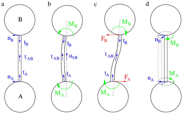
Schematic representation of the mechanical model. a: Two particles, A and B are shown interconnected with a link. At both ends of the link a pair of unit vectors, tA, nA and tB, nB, specify the spatial direction and angular orientation. These direction and orientation vectors co-rotate with the particles attached to the link. The direction of the link at its midpoint between particles A and B is denoted by the unit (tangent) vector tAB. When the link is stress free, tA, tB and tAB, as well as nA and nB are co-linear. b: A symmetric rotation of both particles yields torques MA and MB acting on particles A and B, respectively. These torque vectors are perpendicular to the plane of the figure. The unit vector pointing from particle A to B is denoted by uAB. In this configuration the link does not exert forces perpendicular to uAB as the net torque −(MA +MB) acting on the link is zero. c: A lateral misalignment of the particles creates torques MA, MB and also shear forces FA, FB acting at the particle-link junctions. d: Link torsion is characterized by the angle between the unit vectors nA and nB. A twisted link exert torques that are parallel to the link’s axis. (The link index ℓ is omitted in the figure for better transparency.)
| (2) |
where R is the rotation operator and and denote the neutral link directions in the initial configuration where ϕA = 0.
A link l is bent if its preferred direction at the particle, tA,l, is distinct from its actual direction uAB, the unit vector pointing from particle A to B (Fig. 1b). We assume that the torque exerted by such a link on particle A is
| (3) |
where the microscopic bending rigidity k1 > 0 is a model parameter. Thus, a stress-free (“straight”) link is pointing in a direction tA,l = uAB. In general, the torque (3) rotates particle A so that tA,l aligns with uAB (Figs. 1b and c).
We choose Eq. (3) due to its simplicity. However, a real mechanical system composed of flexible beams would exert similar torques if particles are much smaller than the length of the interconnecting beams, and beams are softer at their ends hence deformations are localized to the vicinity of the particles. In such cases the preferred link direction tA,l is the tangent vector of the link l at the surface of particle A, and the tangent vector at the midpoint, tAB,l, is well approximated by uAB.
Torsion of link l is characterized by two normal vectors, nA,l and nB,l, assigned to each end of the link (Figs. 1a and d). Their specific orientation (normal to the link) is irrelevant, but in the undeformed state nA,l = nB,l. For small deformations the torque is assumed to be proportional to the torsion angle, measured as the angle between the normal vectors as:
| (4) |
where the model parameter k2 > 0 is the microscopic torsional stiffness.
We assume, that in a general situation the net torque of link l acting on particle A is a superposition of the torques associated with bending and torsion:
| (5) |
Similarly, for particle B at the other end of the link l:
| (6) |
where uBA = −uAB.
If a link l exerts forces FA,l and FB,l as well as torques MA,l and MB,l at its endpoints (Fig. 1c), the link is in mechanical equilibrium if
| (7) |
and
| (8) |
To determine the force FA,l = −FB,l, we introduce a unit vector orthogonal both to nA,l and uAB as
| (9) |
We decompose the forces into orthogonal components as
| (10) |
Substituting the composition (10) into Eq. (8) yields
| (11) |
After evaluating the cross products we obtain
| (12) |
hence
| (13) |
and
| (14) |
Finally, is determined by Hook’s law as
| (15) |
where ℓl is the equilibrium length of link l and k3 > 0 is the microscopic elastic modulus, the third model parameter.
Thus, two particles A and B interconnected by link l are characterized by rA, rB, tA,l, nA,l, tB,l, nB,l and ℓ1. Given these quantities, equations (5), (6), (13), (14) and (15) allow the calculation of the 9 components of MA and MB, and of FA = −FB.
2.2. Mechanical equilibrium
A particle may be attached to multiple links and also be the subject of external forces or torques. Net forces
| (16) |
and torques
| (17) |
are calculated by summation over Li, the set of links associated with particle i. In mechanical equilibrium Fi and Mi are zero for each particle i. The equilibrium configuration, however, is difficult to obtain directly due to the nonlinear dependence of the forces on particle positions. Instead, we utilized the following overdamped relaxation process:
| (18) |
and
| (19) |
where Pi and Qi are projector matrices to optionally constrain the movement and rotation of node i, respectively. For unconstrained particles Pi and Qi are identity matrices. As the particles rotate, the unit vectors of neutral link direction and orientation associated to link l and particle i are updated according to (1) and (2).
For a given initial condition, the configuration corresponding to mechanical equilibrium is calculated by solving the coupled ordinary differential equations (18) and (19) by a fourth order Runge-Kutta method. The relaxation was terminated when the magnitude of the net total force and torque in the system fell below a threshold value.
2.3. Initial condition, connectivity
Two dimensional initial conditions were generated by randomly positioning N particles in a square of size . Thus, the spatial scale unit of the simulations is set as the average cell size, d0 ≈10μm and the 2D cell density is 1 cell/unit area. In the initial condition we enforced that the distance of two adjacent particles is greater than dmin = 0.8d0. Particles that are Voronoi neighbors are connected by links when their distance is less than dmax = 2d0. This rule yields a mean link length of ~ 1.2d0. For a stress-free initial configuration we set the vectors as well as the equilibrium link lengths ℓl so that no internal forces or torques are exerted in the system.
2.4. Plasticity
Tissue plasticity is modeled by specific rules that reconfigure the links. As cells can both form new intercellular adhesions and remodel existing ones, in our model the topology of connections changes in time. In particular, we assume that the lifetime of a link is reduced by tensile forces. For a given link l, the probability of its removal during a short time interval Δt follows Bell’s rule [31] as
| (20) |
where F* is a threshold value, and A is a scaling factor which sets the fragility of the connections.
Two adjacent particles (Voronoi neighbors), i and j, can establish new contacts if their distance di,j is less than dmax. During a short time interval Δt, the probability of this event is a decreasing function of the distance:
| (21) |
The scaling factor B represents the level of cellular protrusive activity devoted to scanning the environment and the ability to form intercellular contacts.
Simulations are event-driven: using the probability distributions (20) and (21), we generate the next event μ and waiting time τ according to the stochastic Gillespie algorithm [32]. The waiting time until the next event is chosen from the distribution
| (22) |
where the sums are evaluated using all possible particle pairs i, j not connected by a link as well as enumerating existing links l.
After each event, the system is relaxed into a mechanical equilibrium. A new link is assumed to be stress free immediately after insertion. Cells, however, are expected to maintain a certain area or volume, characterized by the mean stress free link length d0. To reflect this process in our model, the equilibrium length of each link evolves in time according to the stochastic dynamics
| (23) |
where ξ is an uncorrelated white noise with variance σ.
The waiting time between simulation events is set by parameters A and B. We choose our time unit as 1/B ≈ 1s, the time needed for two adjacent cells to establish a mechanical link. In our simulations the time needed for a cell-cell contact to mature is then B/C ≈ 1min. We also set the lifetime of an unloaded link to B/A ≈ 1min, thus two cells pulled away by a force F* separate in ~ 20s.
3. Results
3.1. Elastic parameters
To establish the connection between the macroscopic material parameters such as Young’s modulus and the microscopic model parameters k1, k2 and k3, we simulated elastic deformations in response to uniaxial tension, in-plane shear and (three dimensional) plate bending. The simulations started from a stress-free initial condition and the same microscopic parameters were assigned to each particle. During these simulations the connectivity of the particles and the equilibrium link properties do not change, hence the system exhibits a pure elastic behavior.
In the simulations we use dimensionless quantities, denoted by a tilde. Distances are measured in units of cell size, d0 ≈ 10μm as
| (24) |
We also introduce a force unit F0, which allows to express the microscopic model parameters as dimensionless numbers:
| (25) |
| (26) |
| (27) |
| (28) |
If we choose our force unit as
| (29) |
i.e., the force required to extend a cell twofold along one direction, then according to (28) in the simulations we can set k̃3 = 1.
3.1.1. Uniaxial tension
We applied external, outward-directed forces on particles that are on the left and right side of the test object (Fig. 2a, inset). The external force acting on particle i is
Figure 2.

Simulations of uniaxial stretch. The dimensionless 2D Young’s modulus (E2D/k3; in panel a) and Poisson’s ratio (b) are plotted as a function of the bending rigidity parameter k1/k3. The inset in panel (a) depicts a typical configuration of the stretched sample. Black arrows indicate the external forces prescribed during the simulation. The color of the links indicate compression (red), tension (green) or being at the neutral length d0 (blue). Links in line with the external load are stretched, while those that are oriented in the perpendicular direction are compressed.
| (30) |
Parameters Fleft and Fright are chosen in such a way that the net external force is zero and the magnitude of external forces acting on either side is

| (31) |
After the simulated system reached mechanical equilibrium, we determined the axial elongation ΔL and transverse contraction ΔW. The 2D elastic (Young’s) modulus, E2D, and its dimensionless form
| (32) |
were calculated from the engineering stress and strain as
| (33) |
where a is the slope of a linear fit over the ΔL vs
data points, obtained in the range of 0 <
/F0 < 3.2. Similarly, Poisson’s ratio is obtained as
| (34) |
where b is the slope of a linear fit over the ΔW vs
data points.
Since the deformation is planar, interparticle links do not twist. Therefore, E2D and ν are independent of k2. The bending rigidity parameter k1, however, can substantially influence both material parameters (Fig. 2). For k1 ≪ k3, the external forces are mainly balanced by the elongation of the interparticle links. In this regime thus E2D ≈ k3. Poisson’s ratio is well approximated by 1/[2tg(π/3)] ≈ 0.29, the change in the aspect ratio of a triangular lattice when stretched in one direction while keeping the length unchanged for the rest of lattice links. In contrast, for k1 ≳ k3 bending rigidity of the nodes substantially influences the elastic behavior of the system. Interestigly, ν < 0 for k1 ≫ k3 as link angles are maintained to such an extent that uniaxial stretching will result in an isotropic expansion of the entire mesh. As this regime is biophysically implausible, we restrict the bending rigidity parameter in the
| (35) |
regime.
3.1.2. In-plane shear
In these simulations external shear forces were applied in two layers as
| (36) |
so that the net external force was zero, and the total force is given by (31). To avoid rotation of the simulated system, particles subjected to external forces were also constrained to move along the x axis.
The shear deformation was quantified using the mean displacements Δx of the stripes where forces were acting. The 2D shear modulus was calculated as
| (37) |
where c is the slope of a linear fit over the Δx vs
data points. The obtained shear moduli are well approximated by
| (38) |
the relation expected for an isotropic homogeneous linear elastic solid (Fig. 3).
Figure 3.

The 2D shear modulus, G2D, as obtained from simulations. The green line indicates G = E/2(1 + ν), the relation expected to hold for elastic parameters of a homogenous and isotropic material. The inset depicts a typical configuration of the sheared structure using the color-convention of Fig. 2. Diagonal links are either stretched or compressed, while links oriented either in line with or perpendicular to the direction of shear forces maintain their neutral length.
3.1.3. Bending
To calibrate the bending rigidity of the modeled tissue layer, we simulated a plate immobilized along one side and bent by a perpendicular force exerted at the opposite side. The loading force was localized at the rightmost 10% of the particles, acting in a direction perpendicular to the plane of the particles (Fig. 4).
Figure 4.

Plate bending. a: Macroscopic bending rigidity, EI, vs the microscopic bending rigidity k1 for various values of k2 indicated by red to green colors. The inset depicts a typical simulation configuration. b: The thickness w of a plate that exhibits the same bending and Young’s moduli as presented in panel (a) and Fig. 2a. c,d: Visualization of torques associated with bending (c) and twisting (d) of links, as specified by Eqs (3) and (4), respectively. The configuration shown was obtained in a simulation with k1 = k2 = 0.67k3. Blue to green colors indicate progressively increasing torque magnitudes. Links that are parallel to the loaded edge are twisted, while links oriented to the perpendicular direction are bent.
Simulations revealed that the longitudinal cross section of the deflected monolayer is well approximated by a cubic function – as expected for a beam with finite thickness. Thus, despite the fact that in our model bending rigidity does not arise through the Euler-Bernoulli/Love-Kirchhoff mechanism, we defined and used the modulus EI to relate the deflection z to the loading force
as
| (39) |
This “effective” bending modulus can be tuned over several orders of magnitude, and it is a monotonic, nonlinear function of the microscopic model parameters k1 and k2 (Fig. 4). When torsion of the links is negligible (k2 ≫ k1), the bending modulus EI is proportional to the microscopic bending modulus k1. In contrast, when k2 < k1 the macroscopic curvature of the simulated sheet is mainly accommodated by torsion of the links, hence in this regime EI depends less on the value of k1.
The bending modulus EI also allows one to associate an effective layer thickness w to a set of microscopic model parameters. For a homogenous elastic material of thickness w and the same lateral size L the second moment of the cross-sectional area is
| (40) |
If the stretch data shown in Fig. 2 were measured on the same material with a cross section of wL, then its (three dimensional) Young’s modulus was
| (41) |
Using the bending modulus values EI shown in Fig. 4, and substituting E and I into (39) we obtain
| (42) |
yielding
| (43) |
As an example, the parameters k̃1 = k̃2 = 10−2 are consistent with a w = 3d0 thick plate, or a sheet that is composed of columnar cells with an aspect ratio of 1:3 (Fig. 4b).
These results allow us to further refine the force scale F0. According to Fig. 2, the 2D Young’s modulus is well approximated by k3 in the k1 ≪ k3 regime. The corresponding 3D elastic modulus is then
| (44) |
Thus, (29) can be approximated as
| (45) |
As an example, for the avian epiblast E ≈ 1 kPa [33] and w ≈ 30μm [34], and we obtain
| (46) |
as our force unit.
3.2. Plastic behavior
Link remodeling allows the simulation of elasto-plastic behavior. As the probability of link removal increases when forces are acting on a link, mechanical stresses are thus accommodated and relaxed in an irreversible process. To characterize macroscopic plastic behavior, we simulated two external force-driven processes: force relaxation within a pre-stressed configuration and creep under uniaxial tension. In both scenarios the initial condition involved external forces that pulled longitudinal links with an average force of F0.
3.2.1. Relaxation of mechanical tension
To investigate how the simulated structure can relax mechanical stresses, first an elastic mechanical equilibrium was obtained in the presence of external uniaxial tensile forces distributed according to (30). Then, both sides of the stretched sample were fixed in space by replacing the external forces by stiff springs as
| (47) |
where the parameter k0 = 10k3 sets the stiffness of the constraint and denotes the position of particle i at the onset of the plastic relaxation process. This initial condition was used for the plasticity algorithm that generated a series of link removal and insertion events, each followed by updating the configuration to reflect the new mechanical equilibrium. In each configuration, we evaluated the external forces that were needed to maintain the pre-set extension. As Fig. 5 demonstrates, the net force exerted at either side decays in time as an exponential function to a positive value (the yield stress), and the characteristic time is approximately proportional to the critical force parameter F*. The magnitude of the characteristic time is in a good agreement with the experimental data presented in [13]. During the process particles are rearranged in such a way that the isotropy of link lengths (i.e. cell shape) is restored. The shortening of the longitudinal links was achieved through intercalation: cells in adjacent rows moved into a single row. Hence, in this setting cell intercalation is driven by an external mechanical load. Forces do not diminish completely as the stressed bonds are likely to form again when their removal does not change the local arrangement of the particles substantially.
Figure 5.

The external force required to maintain a pre-set stretch is decreasing in time. A stretched configuration (shown in Fig. 2) served as the initial condition for the simulations. Particles that had been subjected to external fores were fixed in space (marked by rectangles in the inset). The magnitudes of the external forces required to maintain this constraint are shown normalized to their initial, pre-relaxation values. Data were obtained from stochastic simulations with three choices of the force threshold parameter F*. Each data point is an average of three independent simulation runs. Error bars indicate standard deviation. The solid curves are exponential functions with characteristic decay times of τ = 30s (red), 50s (green) and 70s (blue). The inset depicts a late-stage configuration when only 10% of the initial external force is needed to maintain the pre-set constrain.
3.2.2. Creep under constant tension
In a set of complementary simulations the loaded edges were hardened to prevent detachment of the particles. Thus, particles exposed to external forces maintained their orientation by setting Qi to null matrices in Eq. (19) and were connected by more stable links (i.e., links with increased F* parameter). In these simulations the sample gradually extends and narrows (Fig. 6). The initial strain rate is set by the magnitude of the external load and F*. However, as links are removed faster than new ones are inserted, the strain rate increases with time (necking).
Figure 6.

Creep during uniaxial tension. The strain of the sample is plotted as a function of time for three force threshold parameters F*, indicated with distinct colors. Each data point is an average of at least three independent simulation runs. Error bars indicate standard deviation. The inset depicts the configuration after the appearance of necking.
3.3. Cell movements and active cell adhesion control
Model particles can be also considered as simulation agents, executing certain prescribed actions in addition to passively responding to the mechanical forces exerted. Such actions may involve the modulation of link parameters such as the equilibrium link length or the neutral link direction. Furthermore, the probabilities associated with the formation or severance of links may also be controlled. These potential control mechanisms allow the simulation of various cell autonomous behavior and their collective effects.
3.3.1. Active intercalation
Anisotropic cell activities were suggested to drive active intercalation movements of early vertebrate embryos [35]. In our model link removal events allow adjacent particles to rearrange their connections. To model active intercalation we assume that cells are more likely to extend processes and establish intercellular contacts along a selected direction (p). Thus Eq. (21) is expanded as
| (48) |
where 0 ≤ α ≤ 1 is a parameter tuning the strength of anisotropy. Similarly, links perpendicular to p are expected to be less stable, reflected by the modified expression (20)
| (49) |
Simulations performed with orientation-dependent link removal and insertion probabilities (α = 1), and with random cell detachments as a driving mechanism, yield both local cell intercalation and gradual elongation and lateral contraction (i.e., convergent-extension movements) of the tissue (Fig. 7).
Figure 7.

Convergent-extension movements driven by active intercalation. a: initial configuration. b: configuration after 300 link insertion or removal events. c: Particle displacements indicate lateral contraction and axial elongation.
3.3.2. Autocorrelation functions
The spatial and temporal correlations of tissue movements can be used to characterize both simulations (Fig. 8) and empirical data [19]. For an arbitrary quantity ϕ(x, t), temporal autocorrelations are calculated using
Figure 8.

Autocorrelation functions of tissue movements obtained in a system of N = 1100 particles. Temporal (a, c) and spatial (b, d) autocorrelations are plotted for both velocities v (a, b) and velocity fluctuations V (c, d). Velocities are calculated as displacements during a time interval Δt. Data are shown for three time intervals, Δt = 10s (red) 30s (green) and 100s (blue). The linear size of the system was L = 33.
| (50) |
where 〈 … 〉x,t denotes averaging over all possible locations x and time points t. In the nominator of (50) the time points t and t′ are restricted so that their difference falls into a bin B(x) = [x − b; x + b]. Similarly, for spatial autocorrelations we evaluate
| (51) |
Velocities were obtained as
| (52) |
where the Δt time interval is a parameter. Particle velocities, driven by link remodeling events and subsequent relaxation to mechanical equilibrium, exhibit both sustained temporal and long-range spatial correlations (Fig. 8). The latter extend over distances comparable to the size of the simulated system. Correlations increase for velocities calculated with longer Δt values. Hence, instantaneous velocity fields are dominated by mechanical adaptation to random link remodeling events. However, a longer time lag suppresses the noise and the resulting velocity fields are characteristic for the overall tissue movements that are highly correlated both in time and space. Thus, our stochastic simulation rules yield persistent large-scale (multi-cellular) motion patterns.
The presence of a sustained movement pattern motivates to define velocity fluctuations as
| (53) |
where v̄i = 〈vi(t)〉t is the sustained drift velocity of particle i. The velocity fluctuations, mainly adjustments due to changes in connectivity, do not show long range temporal correlations (Fig. 8c). The finite correlation time ~ 2min reflects the link length adjustment rule (23). Velocity fluctuations, however, continue to exhibit long-range spatial correlations (Fig. 8d), due to the strong mechanical coupling within the system.
4. Discussion
4.1. Tissue plasticity
The plastic behavior of cell aggregates was well studied in a series of experiments where aggegates were compressed in an apparatus where both the compression force as well as the shape of the deformed sample could be precisely monitored [13]. Under these circumstances, a short compression elicits an elastic (reversible) deformation. In this elastic regime the deformation is homogenous within the aggregate: individual cells are also compressed along one direction. In contrast, when the compression is maintained for several hours, the force needed to maintain the deformation decreases in time. This decrease is close to exponential, and the behavior is plastic in the sense that after removing the compression force, the aggregate remains in the new equilibrium shape for several hours. Confocal microscopy revealed that cells within the aggregate regained their isotropic shapes – hence they remodeled their intercellular connections. These empirical findings, including the time scale of the plastic relaxation process, are well reproduced by our model (Fig. 5).
Exponential relaxation of shear stress, characteristic for the Maxwell fluid, has been proposed to model embryonic tissues. Such behavior can arise by a sufficient number of cell divisions or apoptoses within the tissue [3], or by a mechanical load-dependent remodeling of intercellular connections [1, 2]. While cell growth, division or death were not considered in our model, the stochastic simulation framework allows their incorporation in future simulations. After assigning probabilities to the distinct event types, the stochastic Gillespie algorithm can generate the events at the correct rate. Cell growth can be taken into account by introducing a time-dependent target length into Eq. (23). In our simulations, in accord with the continuum theory by Preziosi et al [1, 2], the stress does not diminish completely. We attribute this effect to an inherent granularity within the model. A stretched link is replaced in a T1 transition (Fig. 9) by the following sequence of events: 1) a stretched link is removed. 2) The distance between the previously interconnected particles is increased in the new mechanical equilibrium. 3) The resulting “gap” (or soft patch) is filled in by a new link connecting cells in the orthogonal direction. This last step occurs only if the local deformation in step 2 alters distances to an extent that the two particles that were interconnected by the removed link do not remain Voronoi neighbors. Thus, in our model a yield stress, below which the tissue response is elastic, arises naturally.
Figure 9.

Cell neighbor exchange in a T1 transition. a: In the vertex model a polygonal boundary is eliminated, then a new boundary segment forms between cells that were previously non-adjacent. Vertices are represented by filled circles. In the model proposed here a stretched connection between two adjacent cells is removed. As the link was load-bearing, a mechanical equilibrium yields a new configuration where the previously adjacent cells move away, while their neighbors move closer in a direction perpendicular to the direction of the removed link. The central “hole” in the second configuration indicates a soft patch into which adjacent cells can protrude. Finally, a new link can connect previously non-adjacent particles. Particles are represented by open circles, black segments indicate the links between particles. Gray polygons are cell shapes that are not resolved in the model.
4.2. Intercellular forces
Bell’s rule of force-mediated bond dissociation (20) and the corresponding exponential lifetime of adhesion links [31] is supported by dynamic force microscopy experiments [36]. The reported studies indicated a single molecule rupture force (corresponding to F* for a single molecule) around 10 pN. As a cell may display 105 adhesion molecules on its membrane [37], two adjacent cells may be linked by 104 adhesion molecules. Thus, the rupture force needed to separate two cells is 100 nN if we assume that separation breaks each adhesion bond between the two cells. When cells are pulled apart slowly, a much lower force is sufficient as adhesion molecules can spontaneously unbind: for example, embryonic zebrafish cells can be separated by 10 nN forces [24]. In our model the separation of a strained intercellular contact is assumed to be instantaneous (not resolved by the dynamics), we estimate F* ≈ 100nN, which in our force units translates into F* ≈ F0/3, a value used for simulations in Figs. 5–7.
4.3. Model parameters
Our simulation results also shed additional light to the microscopic model parameters k1, k2 and k3. The most straightforward parameter is the spring constant k3 that characterizes the force needed to extend or compress a single cell within the plane of the tissue layer. According to (44), this parameter is determined by the tissue layer’s width and Young’s modulus. For the avian epiblast E ≈ 1 kPa [33] and w ≈ 30μm [34], thus k3 ≈ 30nN/μm.
The microscopic bending rigidity k1 determines the torque Mbend acting on a pair of adherent cells when their configuration is bent within the plane of the tissue layer. To obtain an estimate for k1, let us model the cell pair as a d0 long homogenous, elastic beam with a rectangular cross section of d0 × w. A small deflection at the end of the beam, of the magnitude d0θ, yields a torque
| (54) |
at the other (fixed) end of the beam. Comparing Eqs (3) and (54), for the microscopic bending rigidity we expect
| (55) |
| (56) |
for the value of the dimensionless parameter. For the avian epiblast, k1 ≈ 750 nN·μm.
Similarly, when a cell is rotated by an angle θ relative to its neigbor, the torsion of the cell pair yields a torque
| (57) |
where G = E/2(1 + ν) is the shear modulus and J is the moment of inertia. Assuming the same homogenous beam with a rectangular cross section d0 × w, the moment of inertia is where 0.1 < β < 0.33 is a factor that depends on the aspect ratio of the beam. Comparing (57) and (4), for the microscopic torsion constant we obtain
| (58) |
or in dimensionless form
| (59) |
For the avian epiblast, assuming a Poisson ratio of ν = 0.1, k2 ≈ 360 nN · μm.
While estimates (56) and (59) set the expected magnitude of these parameters, to model a tissue layer of a certain width and Poisson’s ratio, the values of microscope model parameters should be obtained from the more precise simulation results shown in Figs. 2 and 4.
4.4. Tissue movements
The emergence of tissue movements from the collective action of its constituent cells is one of the central questions of developmental biology. Imaging studies established that during later stages of development involving a well-crosslinked matrix the cells and their immediate extracellular matrix surroundings move as a composite material [38, 28], while during earlier stages individual cell motility is superimposed on a larger scale tissue movement [39, 40]. Hence the body plan of early amniote embryos do not appear to be established by “conventional” cell motility – i.e., cells migrating on an external substrate to pre-defined positions following environmental cues. Instead, germ layers and the entire embryo morphology are molded to a large extent by cell-exerted mechanical forces (stresses) and their controlled dissipation/relaxation.
Anisotropic cell behavior has been proposed previously to explain convergent-extension movements [14, 41, 23, 15, 16]. Here we demonstrated that anisotropic cell activity can be formulated within our proposed model, and the simulations yield velocity autocorrelations comparable with those reported for avian embryos [19]. In particular, particle image velocimetry revealed that the displacements of morphogenetic tissue movements are smooth in space and tissue movements are correlated even at locations separated by several hundred micrometers, comparable to the size of the embryo. Velocity vectors, however, strongly fluctuate in time. The autocorrelation time of the velocity fluctuations was reported to be less than a minute. Our model suggest that fluctuations with a short correlation time can be generated by sudden cellular detachment/reattachment events occurring at random positions – the driving mechanism of tissue movements. The long correlation length is consistent with the idea that the tissue is in mechanical equilibrium, therefore a local change in cell traction is expected to immediately alter tissue deformations elsewhere.
In summary, we demonstrated that the proposed model yields a realistic elasto-plastic behavior with exponential relaxation of tensile stresses above an intrinsic threshold value. Due to the simplicity of the model, microscopic parameter values can be inferred from tissue thickness, its macroscopic elastic modulus and Poisson’s number and the magnitude and dynamics of intercellular adhesion forces. The proposed stochastic simulation of cell activities gives rise to fluctuating tissue movements, which exhibit the same autocorrelation properties as the empirically obtained data. This model, therefore, can serve as a mechanically correct basis for cell-resolved or agent-based future studies focusing on tissue morphogenesis.
Acknowledgments
This work was supported by the NIH (grant HL085694 to Dr Brenda Rongish), the Hungarian Development Agency (KTIA AIK 12-1-2012-0041), the Hungarian Research Fund (OTKA K72664) and the G. Harold & Leila Y. Mathers Charitable Foundation. We are most grateful for Drs Sandra Rugonyi, Brenda Rongish and Charles Little for fruitful discussions and comments on the manuscript.
References
- 1.Preziosi L, Ambrosi D, Verdier C. An elasto-visco-plastic model of cell aggregates. J Theor Biol. 2010 Jan;262(1):35–47. doi: 10.1016/j.jtbi.2009.08.023. [DOI] [PubMed] [Google Scholar]
- 2.Preziosi L, Vitale G. A multiphase model of tumor and tissue growth including cell adhesion and plastic reorganization. Mathematical Models and Methods in Applied Sciences. 2011 Sep;21(09):1901–1932. [Google Scholar]
- 3.Ranft J, Basan M, Elgeti J, Joanny JF, Prost J, Julicher F. Fluidization of tissues by cell division and apoptosis. Proc Natl Acad Sci U S A. 2010 Dec;107(49):20863–20868. doi: 10.1073/pnas.1011086107. [DOI] [PMC free article] [PubMed] [Google Scholar]
- 4.Giverso C, Preziosi L. Modelling the compression and reorganization of cell aggregates. Math Med Biol. 2012 Jun;29(2):181–204. doi: 10.1093/imammb/dqr008. [DOI] [PubMed] [Google Scholar]
- 5.Fung YC. Biomechanics: mechanical properties of living tissues. Springer-Verlag; New York: 1993. [Google Scholar]
- 6.Stolarska MA, Kim Y, Othmer HG. Multi-scale models of cell and tissue dynamics. Philos Trans A Math Phys Eng Sci. 2009 Sep;367(1902):3525–3553. doi: 10.1098/rsta.2009.0095. [DOI] [PMC free article] [PubMed] [Google Scholar]
- 7.Taber LA. Towards a unified theory for morphomechanics. Philos Transact A Math Phys Eng Sci. 2009 Sep;367(1902):3555–3583. doi: 10.1098/rsta.2009.0100. [DOI] [PMC free article] [PubMed] [Google Scholar]
- 8.Varner VD, Voronov DA, Taber LA. Mechanics of head fold formation: investigating tissue-level forces during early development. Development. 2010 Nov;137(22):3801–3811. doi: 10.1242/dev.054387. [DOI] [PMC free article] [PubMed] [Google Scholar]
- 9.Graner F, Glazier JA. Simulation of biological cell sorting using a two-dimensional extended potts model. Phys Rev Lett. 1992 Sep;69(13):2013–2016. doi: 10.1103/PhysRevLett.69.2013. [DOI] [PubMed] [Google Scholar]
- 10.Izaguirre JA, Chaturvedi R, Huang C, Cickovski T, Coffland J, Thomas G, Forgacs G, Alber M, Hentschel G, Newman SA, Glazier JA. Compucell, a multi-model framework for simulation of morphogenesis. Bioinformatics. 2004;20(7):1129–1137. doi: 10.1093/bioinformatics/bth050. [DOI] [PubMed] [Google Scholar]
- 11.Newman TJ. Modeling multicellular systems using subcellular elements. Math Biosci Eng. 2005;2:611–622. doi: 10.3934/mbe.2005.2.613. [DOI] [PubMed] [Google Scholar]
- 12.Sandersius SA, Chuai M, Weijer CJ, Newman TJ. Correlating cell behavior with tissue topology in embryonic epithelia. PLoS One. 2011;6(4):e18081. doi: 10.1371/journal.pone.0018081. [DOI] [PMC free article] [PubMed] [Google Scholar]
- 13.Forgacs G, Foty RA, Shafrir Y, Steinberg MS. Viscoelastic properties of living embryonic tissues: a quantitative study. Biophys J. 1998;74(5):2227–2234. doi: 10.1016/S0006-3495(98)77932-9. [DOI] [PMC free article] [PubMed] [Google Scholar]
- 14.Zajac M, Jones GL, Glazier JA. Model of convergent extension in animal morphogenesis. Phys Rev Lett. 2000;85:2022–5. doi: 10.1103/PhysRevLett.85.2022. [DOI] [PubMed] [Google Scholar]
- 15.Vasiev B, Balter A, Chaplain M, Glazier JA, Weijer CJ. Modeling gastrulation in the chick embryo: formation of the primitive streak. PLoS One. 2010;5(5):e10571. doi: 10.1371/journal.pone.0010571. [DOI] [PMC free article] [PubMed] [Google Scholar]
- 16.Sandersius SA, Chuai M, Weijer CJ, Newman TJ. A ‘chemotactic dipole’ mechanism for large-scale vortex motion during primitive streak formation in the chick embryo. Phys Biol. 2011 Aug;8(4):045008. doi: 10.1088/1478-3975/8/4/045008. [DOI] [PubMed] [Google Scholar]
- 17.Christley S, Lee B, Dai X, Nie Q. Integrative multicellular biological modeling: a case study of 3d epidermal development using gpu algorithms. BMC Syst Biol. 2010;4:107. doi: 10.1186/1752-0509-4-107. [DOI] [PMC free article] [PubMed] [Google Scholar]
- 18.Gord A, Holmes WR, Dai X, Nie Q. Computational modelling of epidermal stratification highlights the importance of asymmetric cell division for predictable and robust layer formation. J R Soc Interface. 2014 Oct;11(99) doi: 10.1098/rsif.2014.0631. [DOI] [PMC free article] [PubMed] [Google Scholar]
- 19.Szabó A, Rupp PA, Rongish BJ, Little CD, Czirók A. Extracellular matrix fluctuations during early embryogenesis. Phys Biol. 2011 Aug;8(4):045006. doi: 10.1088/1478-3975/8/4/045006. [DOI] [PMC free article] [PubMed] [Google Scholar]
- 20.Honda H, Eguchi G. How much does the cell boundary contract in a monolayered cell sheet? J Theor Biol. 1980 Jun;84(3):575–588. doi: 10.1016/s0022-5193(80)80021-x. [DOI] [PubMed] [Google Scholar]
- 21.Fletcher AG, Osterfield M, Baker RE, Shvartsman SY. Vertex models of epithelial morphogenesis. Biophys J. 2014 Jun;106(11):2291–2304. doi: 10.1016/j.bpj.2013.11.4498. [DOI] [PMC free article] [PubMed] [Google Scholar]
- 22.Farhadifar R, Rper JC, Aigouy B, Eaton S, Jlicher F. The influence of cell mechanics, cell-cell interactions, and proliferation on epithelial packing. Curr Biol. 2007 Dec;17(24):2095–2104. doi: 10.1016/j.cub.2007.11.049. [DOI] [PubMed] [Google Scholar]
- 23.Rauzi M, Verant P, Lecuit T, Lenne PF. Nature and anisotropy of cortical forces orienting drosophila tissue morphogenesis. Nat Cell Biol. 2008 Dec;10(12):1401–1410. doi: 10.1038/ncb1798. [DOI] [PubMed] [Google Scholar]
- 24.Maitre JL, Berthoumieux H, Krens SFG, Salbreux G, Jlicher F, Paluch E, Heisenberg CP. Adhesion functions in cell sorting by mechanically coupling the cortices of adhering cells. Science. 2012 Oct;338(6104):253–256. doi: 10.1126/science.1225399. [DOI] [PubMed] [Google Scholar]
- 25.Honda H, Tanemura M, Nagai T. A three-dimensional vertex dynamics cell model of space-filling polyhedra simulating cell behavior in a cell aggregate. J Theor Biol. 2004 Feb;226(4):439–453. doi: 10.1016/j.jtbi.2003.10.001. [DOI] [PubMed] [Google Scholar]
- 26.Drasdo D, Forgacs G. Modeling the interplay of generic and genetic mechanisms in cleavage, blastulation, and gastrulation. Dev Dyn. 2000 Oct;219(2):182–191. doi: 10.1002/1097-0177(200010)219:2<182::aid-dvdy1040>3.3.co;2-1. [DOI] [PubMed] [Google Scholar]
- 27.Ramis-Conde I, Drasdo D, Anderson ARA, Chaplain MAJ. Modeling the influence of the e-cadherin-beta-catenin pathway in cancer cell invasion: a multiscale approach. Biophys J. 2008 Jul;95(1):155–165. doi: 10.1529/biophysj.107.114678. [DOI] [PMC free article] [PubMed] [Google Scholar]
- 28.Aleksandrova A, Czirok A, Szabo A, Filla MB, Hossain MJ, Whelan PF, Lansford R, Rongish BJ. Convective tissue movements play a major role in avian endocardial morphogenesis. Dev Biol. 2012 Mar;363(2):348–361. doi: 10.1016/j.ydbio.2011.12.036. [DOI] [PMC free article] [PubMed] [Google Scholar]
- 29.Cui C, Little CD, Rongish BJ. Rotation of organizer tissue contributes to left-right asymmetry. Anat Rec (Hoboken) 2009 Apr;292(4):557–561. doi: 10.1002/ar.20872. [DOI] [PMC free article] [PubMed] [Google Scholar]
- 30.Gros J, Feistel K, Viebahn C, Blum M, Tabin CJ. Cell movements at hensen’s node establish left/right asymmetric gene expression in the chick. Science. 2009 May;324(5929):941–944. doi: 10.1126/science.1172478. [DOI] [PMC free article] [PubMed] [Google Scholar]
- 31.Bell GI. Models for the specific adhesion of cells to cells. Science. 1978 May;200(4342):618–627. doi: 10.1126/science.347575. [DOI] [PubMed] [Google Scholar]
- 32.Gillespie DT. Exact stochastic simulation of coupled chemical reactions. The Journal of Physical Chemistry. 1977;81(25):2340–2361. [Google Scholar]
- 33.Agero U, Glazier JA, Hosek M. Bulk elastic properties of chicken embryos during somitogenesis. Biomed Eng Online. 2010;9:19. doi: 10.1186/1475-925X-9-19. [DOI] [PMC free article] [PubMed] [Google Scholar]
- 34.Bellairs R, Osmond M. The atlas of chick development. Academic Press; San Diego, CA: 1998. [Google Scholar]
- 35.Voiculescu O, Bertocchini F, Wolpert L, Keller RE, Stern CD. The amniote primitive streak is defined by epithelial cell intercalation before gastrulation. Nature. 2007 Oct;449(7165):1049–1052. doi: 10.1038/nature06211. [DOI] [PubMed] [Google Scholar]
- 36.Zhang X, Craig SE, Kirby H, Humphries MJ, Moy VT. Molecular basis for the dynamic strength of the integrin alpha4beta1/vcam-1 interaction. Biophys J. 2004 Nov;87(5):3470–3478. doi: 10.1529/biophysj.104.045690. [DOI] [PMC free article] [PubMed] [Google Scholar]
- 37.Foty RA, Steinberg MS. Cadherin-mediated cell-cell adhesion and tissue segregation in relation to malignancy. Int J Dev Biol. 2004;48(5–6):397–409. doi: 10.1387/ijdb.041810rf. [DOI] [PubMed] [Google Scholar]
- 38.Benazeraf B, Francois P, Baker RE, Denans N, Little CD, Pourquie O. A random cell motility gradient downstream of fgf controls elongation of an amniote embryo. Nature. 2010 Jul;466(7303):248–252. doi: 10.1038/nature09151. [DOI] [PMC free article] [PubMed] [Google Scholar]
- 39.Zamir EA, Czirok A, Cui C, Little CD, Rongish BJ. Mesodermal cell displacements during avian gastrulation are due to both individual cell-autonomous and convective tissue movements. Proc Natl Acad Sci U S A. 2006 Dec;103(52):19806–19811. doi: 10.1073/pnas.0606100103. [DOI] [PMC free article] [PubMed] [Google Scholar]
- 40.Zamir EA, Rongish BJ, Little CD. The ecm moves during primitive streak formation–computation of ecm versus cellular motion. PLoS Biol. 2008 Oct;6(10):e247. doi: 10.1371/journal.pbio.0060247. [DOI] [PMC free article] [PubMed] [Google Scholar]
- 41.Zajac M, Jones GL, Glazier JA. Simulating convergent extension by way of anisotropic differential adhesion. J Theor Biol. 2003;222(2):247–259. doi: 10.1016/s0022-5193(03)00033-x. [DOI] [PubMed] [Google Scholar]