

Abstract
BACKGROUND
The United Nations (UN) produces population projections for all countries every two years. These are used by international organizations, governments, the private sector and researchers for policy planning, for monitoring development goals, as inputs to economic and environmental models, and for social and health research. The UN is considering producing fully probabilistic population projections, for which joint probabilistic projections of future female and male life expectancy at birth are needed.
OBJECTIVE
We propose a methodology for obtaining joint probabilistic projections of female and male life expectancy at birth.
METHODS
We first project female life expectancy using a one-sex method for probabilistic projection of life expectancy. We then project the gap between female and male life expectancy. We propose an autoregressive model for the gap in a future time period for a particular country, which is a function of female life expectancy and a t-distributed random perturbation. This method takes into account mortality data limitations, is comparable across countries, and accounts for shocks. We estimate all parameters based on life expectancy estimates for 1950–2010. The methods are implemented in the bayesLife and bayesPop R packages.
RESULTS
We evaluated our model using out-of-sample projections for the period 1995–2010, and found that our method performed better than several possible alternatives.
CONCLUSIONS
We find that the average gap between female and male life expectancy has been increasing for female life expectancy below 75, and decreasing for female life expectancy above 75. Our projections of the gap are lower than the UN’s 2008 projections for most countries and so lead to higher projections of male life expectancy.
1 Introduction
Every two years, the Population Division of the United Nations (UN) publishes the World Population Prospects (WPP), reporting population estimates and projections for all countries. Experts then use these projections to monitor population trends and as inputs to economic and environmental models. The UN’s population projections form the basis of many nations’ and regions’ development plans (Heilig et al., 2010).
Since 1980, each edition of the WPP has included three projection variants: low, medium and high. The medium variant is intended to represent the most likely population size given past trends and expert knowledge. The low and high variants are then generated using different fertility assumptions: total fertility is taken to be half a child either below or above that used to generate the medium scenario. Thus the variation in fertility allowed by this method is insensitive to either the level of fertility in a particular country or its trend. The assumptions about mortality and international migration are the same in all three variants.
Deterministic population projections are unable to fully take into account the variability in demographic processes across countries or to indicate a range of future population outcomes. As a result, the UN is considering issuing probabilistic population projections as an alternative to their standard variants of deterministic projections. Since WPP projections are based on the cohort-component method, probabilistic projections of the main demographic processes affecting national populations (fertility, mortality and international migration) are required to produce probabilistic population projections for all countries.
Probabilistic projections of fertility for all countries have already been developed by Alkema et al. (2011) and implemented in WPP 2010 (United Nations, 2011). The medium variant in WPP 2010 corresponds to the median of the many possible future fertility paths for each country generated by the Alkema et al. (2011) model.
Here we are concerned with the projection of mortality. The simplest method of forecasting mortality is to project life expectancy and use either recent mortality patterns or model life tables to obtain the age pattern required for use in cohort-component methods (Booth, 2006). Given missing and frequently inaccurate data for many countries, this method is used by the UN for most countries.
A probabilistic approach to projecting life expectancy for males has been developed by Raftery et al. (2013) and is an extension of the UN’s current method. It models life expectancy in a country as a random walk with a nonconstant drift, where the drift term is a nonlinear function of current life expectancy and reflects varying rates of improvement for countries at different levels of life expectancy. The use of a Bayesian hierarchical model (BHM) allows for the estimation of the rate of improvement in life expectancy for a country using past data from that country, while also taking into account observed patterns in other countries. The same model can be used for female life expectancy.
The BHM of Raftery et al. (2013) has the disadvantage that it models life expectancy for one sex only, and disregards the relationship between male and female life expectancies. Thus, like many other mortality forecasting models (Bongaarts, 2009; Cairns et al., 2011; Haberman & Renshaw, 2008; Hyndman & Shahid Ullah, 2007; Shang et al., 2011; Soneji & King, 2011), it does not produce joint projections of male and female life expectancy. These are required to obtain fully probabilistic projections of life expectancy for both sexes and to avoid crossovers that are not expected to occur in the future. Girosi & King (2008) proposed a general approach to projecting age-specific mortality rates that could in principle be used for this problem, but they did not describe an explicit method for doing so.
Li & Lee (2005) have proposed a method for forecasting mortality for both sexes in a country using the augmented common factor model, which is a general method for achieving coherence between the mortality rates of different groups (in this case the two sexes in a population) that are expected not to diverge. Hyndman et al. (2013) extended this to explicitly model the smoothness of mortality rates with respect to age, using the product-ratio functional method.
Here we propose a method for joint probabilistic projection of male and female life expectancy that ensures coherence between them in a simple manner: by projecting the gap between them. The gap is defined as female life expectancy minus male life expectancy, and is thus positive in most cases. Projections of female life expectancy are generated by the BHM, and are then combined with projections of the gap to produce projections of male life expectancy.
In focusing on the gap in life expectancy between females and males, this paper adds to a large body of literature studying comparative mortality patterns of the two sexes. Several explanations have emerged for the difference in patterns, from the biological to the behavioral and socioeconomic (Elo & Drevenstedt, 2005; Pampel, 2005; Rogers et al., 2010; Trovato & Lalu, 1998; Trovato & Heyen, 2006; Trovato & Lalu, 2007). In addition, many have commented on the recent narrowing of the gap in high-income countries (Bobak, 2003; Conti et al., 2003; Emslie & Hunt, 2008; Glei & Horiuchi, 2007; Gómez-Redondo & Boe, 2005; Kołodziej et al., 2008; Meslé, 2004; Pampel, 2005; Preston & Wang, 2006; Trovato & Lalu, 1996; Trovato & Odynak, 2011; Staetsky, 2009; Staetsky & Hinde, 2009).
While several authors have provided opinions about the probable trajectory of the gap in high-income countries (Meslé, 2004; Rogers et al., 2010; Trovato & Lalu, 2007), few have attempted to make explicit projections (Pampel, 2005; Preston & Wang, 2006). When they did so, they focused on data-rich high-income countries. We are aware of only two studies that study the gap in life expectancy in developing countries: they show that conflicts (Plümper & Neumayer, 2006) and natural disasters (Neumayer & Plümper, 2007) have different effects on the life expectancy of the two sexes, and thus affect the gap between them.
We propose to model the gap in life expectancy between females and males for all the countries that are not in the midst of a generalized HIV/AIDS epidemic. After briefly discussing the data we use, we describe the model. Next, we assess the performance of our model and possible competing models using data from 1950–1995 to project life expectancy over the period 1995–2010. We then discuss our projections for four countries chosen as examples of possible future trends in the gap between female and male life expectancy: continued decline in the gap for a country in which the decline has already been observed (Ireland), decline in the gap for a country in which the decline has not yet been observed (Guatemala), continued rise, followed by a decline (Laos), and continued rise over the projection period (Cambodia). We conclude with a discussion of the merits and limitations of our method.
2 Data
We use the WPP 2008 estimates of past life expectancy from 1950 to 2010 for all the countries in the world (United Nations, 2009). We compare our projections with the WPP 2008 projections of life expectancy for the period 2010–2050. These data and projections are included in the R package wpp2008 (Ševčíková & Gerland, 2014).
It is widely recognized that mortality data for many countries are incomplete and have inaccuracies. Indeed, according to the 2005 UN World Mortality Report, since 1990, only 56% of the 196 countries with 100,000 inhabitants or more in 2009 have “reliable” or “fairly reliable” vital statistics for adult mortality, and 7% of countries completely lack recent data for the estimation of adult mortality. Countries for which data are unreliable are concentrated mostly in Africa and Asia, and include 91% of countries in Africa and 44% of countries in Asia.
Mortality patterns are significantly affected by the HIV/AIDS epidemic, which has been a major source of mortality in the last twenty years and has predominantly affected young or middle-aged adults, unlike most other causes of death. As a result, we exclude countries with a generalized HIV/AIDS epidemic, as defined by the Joint United Nations Programme on HIV/AIDS (UNAIDS). We also exclude small countries with a population of 100,000 or less. We therefore concentrate on 158 countries with 100,000 inhabitants or more in 2009 and no generalized HIV/AIDS epidemic. These accounted for 89.2% of the world population in 2009.
The data for male and female life expectancy at birth in these 158 countries for the period 1950–2010 are shown in Figure 1. We note several patterns: both male and female life expectancy at birth have been increasing over time, with median female life expectancy in the last period (76.5 years) being higher than male (70.9 years). The between-country variability has decreased over time. The median gap between female and male life expectancy increased from 1950–1955 to 1990–1995, with a slight decline thereafter.1 In 2005–2010, the median gap in life expectancy was 4.9 years, with an interquartile range of (3.9, 6.6). The between-country variability in the gap in life expectancy has declined over time. However, in each quinquennium, at least one country had a gap that was extreme relative to the other countries. The presence of outliers must therefore be taken into account when projecting the gap in future periods.
Figure 1.
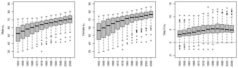
Trends in male and female life expectancy at birth (e0) and the gap between them for all 158 countries under study over the period 1950–2010, based on estimates in WPP 2008. The dark lines in the boxplots indicate median values; the gray boxes extend to the first and third quartile, and the whiskers extend to the most extreme data point which is no more than 1.5 times the interquartile range from the box. Each quinquennium is identified by its middle year (e.g. 1950–1955 → 1953).
Figure 2 displays the narrowing of the gap in life expectancy between the sexes that has been reported in the literature for high-income countries — we use membership of the Organization for Economic Cooperation and Development (OECD) as a distinguishing trait. The trend is not present in non-OECD countries, though some, including Brazil and Uruguay, have experienced lower levels of the gap at higher levels of female life expectancy. Figure 2 also shows that the trend in the gap is more easily seen when plotted against female life expectancy than against time.
Figure 2.

Trends in the gap between female and male life expectancy at birth for OECD (right panels) and non-OECD countries (left panels) over time (top panels) and over female life expectancy at birth (bottom panels) for 1950–2010 as reported in WPP 2008. The red lines show a loess smooth of the data points. The trend in the gap for five countries is shown for illustration: Bhutan, Brazil, Italy, United States and Uruguay.
3 Methodology
Until the 2010 revision of the World Population Prospects, the UN projected female and male life expectancy independently and deterministically, using point forecasts from the method of Lee & Carter (1992), with a modification to ensure that projections for the two sexes do not diverge (Li & Lee, 2005).
3.1 Review of the One-Sex Bayesian Hierarchical Model for Life Expectancy
The BHM of Raftery et al. (2013), which we now briefly summarize, is a one-sex model. Female life expectancy at birth for country c in five-year period t, denoted by , is assumed to follow a random walk with drift, given by
| (1) |
where , with a smooth declining function of . In equation (1), the expected five-year gain in life expectancy is a double-logistic function of the current level of life expectancy, namely
| (2) |
where are the six parameters of the double-logistic function for country c, and A1 and A2 are constants.
Each of the parameters of the double-logistic function for country c is in turn assumed to be drawn from a world distribution of the parameter:
| (3) |
| (4) |
| (5) |
where Normal[a,b](μ, σ2) denotes a normal distribution with mean μ and standard deviation σ, truncated to lie between a and b, and the ai and bi are constants. The world parameters in equations (3)–(5) are assigned prior distributions. The resulting Bayesian hierarchical model is estimated by Markov chain Monte Carlo, yielding a large sample from the joint posterior distribution of all parameters in the model. More details are given in Raftery et al. (2013).
3.2 Modeling the Gap
To obtain joint probabilistic projections of female and male life expectancy, we need to model the relationship between the two. We do this by projecting the gap in life expectancy by linear regression using female life expectancy as a covariate.
The pattern of decline in the gap in life expectancy has been observed only for high-income countries, and for some emerging economies. The question then arises: should we project that other countries will also follow this pattern? Vallin (2005) argued that there is no reason why the experience of English-speaking countries and Scandinavian countries (now extended to most high-income countries) should not become generalized, enabling men in most places to eventually regain some of the ground they lost during the 20th century. Bongaarts (2009) agreed that mortality patterns observed for high-income countries will most likely be followed by others: “There is an expectation that, as developing countries evolve, they will also get rid of non-senescent mortality, since non-senescent deaths unrelated to aging (e.g., accidents, certain infections) can be avoided by effective public health and safety measures and through medical intervention.”
We note also in Figure 2 that non-OECD countries have much lower female life expectancy than OECD countries, and it is only at high levels of female life expectancy that a narrowing in the sex gap has been observed. Thus, it is plausible that the reversal has not yet been seen in most non-OECD countries simply because they have not yet reached the female life expectancy level at which the gap begins to narrow.
Between 1950 and 2010, several countries experienced events that have had a significant impact on the gap between female and male life expectancy. The gap in Bosnia and Herze-govina increased gradually from 2.2 to 5.3 years between 1950–1955 and 1985–1990, then jumped to 17.3 years in 1990–1995 during a period of conflict before falling to 5.4 years in the next quinquennium. Similarly, the gap in Iraq increased from 6.3 years in 1980–1985 to 12.7 years in 1985–1990, and remained at approximately that level until the 1995–2000 quinquennium, when it dropped to 5.6 years. Because we can expect such shocks to continue to occur in the future, we must allow for outliers in our model.
Ours is not the first attempt to deal with outliers in mortality data. Hyndman & Shahid Ullah (2007) used robust statistics in developing their method for forecasting age-specific mortality and fertility rates observed over time. However, while their objective was to identify and remove data associated with extreme events, ours is to incorporate them in our projections so as to more realistically capture perturbations that may occur in the future.
In order to allow for outliers in our projections, we use the t-distribution rather than the normal distribution to model random perturbations, and we estimate the parameters of the t-distribution, including the number of degrees of freedom, using the maximum likelihood method of Lange et al. (1989) and Taylor & Verbyla (2004). We found that the t-distribution tended to generate outliers similar qualitatively to those observed in the data, but also occasionally generated very large outliers of much greater magnitude than any observed in the data. As a result, we truncated the predictive distribution, with the truncation points estimated from the data. This gave a model that yielded outlying values of the gap similar to those observed historically, but not very extreme outliers beyond the range of experience.
To produce joint probabilistic projections of female and male life expectancy, we project the gap in life expectancy by simulating a large number of future trajectories from a linear regression model with BHM female life expectancy projections as a covariate. For each simulated value of the gap, we subtract it from a simulated value of female life expectancy projection to obtain the corresponding simulated male life expectancy projection. The result is a large number of (female e0, male e0) pairs, which form a sample from the joint predictive distribution sought.
We use female rather than male life expectancy as a basis for projecting the gap because female life expectancy tends to be more stable and more accurately measured. For comparison purposes, however, we also build a model for the gap using male life expectancy projections from the BHM for comparison.
Our proposed model for the gap in life expectancy at birth between females and males represents the gap, Gc,t for country c in the current quinquennium, t, as a linear combination of four terms. These are: the gap in the previous quinquennium, Gc,t−1; female life expectancy at birth in the first quinquennium in our dataset (1950–1955), ; female life expectancy at birth in the current quinquennium, ; and the number of years by which exceeds τ, namely , where we use the notation (x)+ = x if x > 0 and 0 otherwise. The quantity τ is the level of female life expectancy at which the gap is expected to stop widening and to start narrowing. Finally, at the highest observed levels of female life expectancy and beyond, denoted by ages A and greater, the gap is modeled as a random walk with normally distributed changes and no drift. This is because we have little information on the determinants of changes in the gap at these high ages and we have observed no outliers for the countries with the highest current life expectancies.
In summary, our model is as follows:
where
where
Estimates of the parameters of this model based on data from 158 countries for 1950–2010 contained in WPP 2008 were obtained by maximum likelihood and are reported in Table 1. The maximum likelihood estimates of L and U are the minimum and maximum observed gaps respectively, namely L̂ = −2.67 and Û = 17.34. Given these values, all the for the historical data period are observed. Conditionally on τ and A, the model for the is thus a linear regression model with t-distributed errors, and we estimated it from the historical data by maximum likelihood using the R package hett (Taylor, 2009). We then maximized the resulting maximum likelihoods over integer values of τ and A to obtain overall maximum likelihoods. The resulting estimates were τ = 75 years and A = 83 years. While slight heteroscedasticity was observed, we chose not to model it explicitly so as to keep the model as simple as possible. Also, the original estimate of the degrees of freedom parameter was 2.07 (standard error 0.13), which we rounded down to 2, again for simplicity.
Table 1.
Estimates and Standard Errors of Parameters used in Gap Projection Model
| Parameter | Estimate | Standard Error |
|---|---|---|
| β0 | −0.2680 | 0.0648 |
| β1 | 0.0056 | 0.0011 |
| β2 | 0.9533 | 0.0044 |
| β3 | 0.0056 | 0.0013 |
| β4 | −0.0851 | 0.0053 |
| σ(1) | 0.2572 | |
| σ(2) | 0.4199 | |
| τ | 75 | |
| A | 83 | |
| L | −2.67 | |
| U | 17.34 |
This model represents the empirical regularities in the data in a simple way. The gap in five-year period t, Gc,t depends on the gap in period t −1, Gc,t−1, reflecting the fact that the gap evolves over time in a somewhat smooth way. Our estimate of β2 was highly significantly positive and our estimate of β4 was highly significantly negative, with p values less than 10−5 in both cases. Thus the gap increases with female life expectancy for female life expectancy up to about age 75, and decreases thereafter up to about age 83; this reflects the pattern seen in the lower right panel of Figure 2. Beyond that our data are too sparse to provide evidence for anything other than a random walk without drift. The model is illustrated in Figure 3, showing the expected evolution of the gap over 150 years from 1950 to 2100, for a country with female life expectancy at birth of 40 and a gap of 3 years in 1950, conditional on an assumed typical evolution of female life expectancy over the period.
Figure 3.

Illustration of the Model for the Gap in Life Expectancy. Left panel: Expected evolution of the gap in life expectancy as a function of female life expectancy. Right panel: Expected evolution of female and male life expectancy over the period 1950–2100. Both are for a hypothetical country with female life expectancy at birth of 40 and a gap of 3 years in 1950, and are conditional on an assumed typical evolution of female life expectancy over the period.
This pattern of a gap that increases and then decreases reflects the data and seems plausible in other ways as well. Higher female life expectancy is associated to some extent with lower and later fertility (Maklakov, 2008; Müller et al., 2002), and the increasing gap corresponds roughly to the demographic transition involving decreasing fertility, so this may be one factor explaining the initial increase in the gap.
In populations with medium life expectancy, men are typically exposed to higher risk than women in midlife, such as dangerous physical jobs and riskier lifestyles (smoking, drinking, physical risk-taking), leading to a higher gap in life expectancy. In countries with high life expectancy, infant and child mortality is low for both sexes and hence quite similar for males and females, and differences in life expectancy are due at least partly to different lifestyles of men and women (Gjonça et al., 1999; Waldron, 1995). These lifestyles may become more similar over time, partly explaining why the gap in life expectancy is closing past a certain level of longevity.
Beyond female life expectancy of A = 83 years, our model does not project further linear declines in the gap, since we have few data on which to base projections. A continued decline in the gap would imply that the gap would eventually become negative in all countries, with high probability. However, several authors have noted that there may be biological reasons why this would be unlikely (Austad, 2011; Soliani & Lucchett, 2006; Vallin, 2006), including the protective effect of oestrogen (Lord et al., 2010), adverse effects of testosterone (Bassil & Morley, 2010) and women’s more robust immune systems (Owens, 2002; Falagas et al., 2008).
The overall level of the gap is also positively related to female life expectancy at the beginning of our data in 1950. Finally, this is a linear regression model with t distributed errors. The t distribution has longer tails and generates more outliers than the normal distribution, and so this model allows for the occasional extreme values that we observe in the data.
The overall method for joint probabilistic projection of female and male life expectancy is implemented in the bayesLife R package (Ševčíková & Raftery, 2014), for which a GUI is provided by the bayesDem R package (Ševčíková, 2013).
4 Model Validation
In order to assess the performance of our model, we estimated model parameters based on the data from 1950 to 1995 only, containing 1,422 country-period combinations, and we then forecast the gap in life expectancy from 1995 to 2010. We then compared our results to WPP 2008 estimates of the gap for those three quinquennia. This yielded 474 out-of-sample projections.
We assessed three attributes of our model: calibration, precision, and accuracy. An ideal model is calibrated (i.e. an x% prediction interval covers the true value x% of the time on average), precise (i.e. its prediction intervals are narrow), and accurate (i.e. it makes small errors in prediction). We measured accuracy by reporting the mean absolute error of the median of the probabilistic projections.
We also compared the performance of our model to other potential gap projection methods. For the gap in life expectancy, we compared the performance of the gap model based on female life expectancy to the gap model based on the male life expectancy, as well as to the difference between independent projections of female and male life expectancy under the BHM, constrained to the range [−3, 18] (“BHM Projection”). We also report the accuracy of a model that assumes that the gap would remain at 1990–1995 levels from 1995 to 2010 (“Constant 1995 Gap”). Our results are shown in Table 2.
Table 2.
Results for 15-year out-of-sample cross-validation for four different projection models for 1) the gap between female and male life expectancy at birth, 2) male life expectancy at birth, and 3) female life expectancy at birth.
| Calibration and Precision of the Prediction Interval | Accuracy of the Prediction | ||||
|---|---|---|---|---|---|
| Coverage | Avg. Half-Width | Mean Absolute Error | |||
| 80% | 95% | 80% | 95% | ||
| GAP IN e0 | |||||
| UN Model (simulated) | – | – | – | – | 0.78 |
| Constant 1995 Gap | – | – | – | – | 0.73 |
| BHM Projection | 0.80 | 0.92 | 1.57 | 2.40 | 0.78 |
| Male e0-based Model | 0.68 | 0.93 | 0.75 | 1.57 | 0.70 |
| Female e0-based Model | 0.73 | 0.94 | 0.76 | 1.58 | 0.66 |
| MALE e0 | |||||
| UN Model (simulated) | – | – | – | – | 2.32 |
| Constant 1995 Gap | 0.64 | 0.85 | 1.61 | 2.46 | 1.42 |
| BHM Projection | 0.79 | 0.94 | 2.05 | 3.13 | 1.44 |
| Gap-based Model | 0.76 | 0.93 | 1.90 | 3.02 | 1.32 |
| FEMALE e0 | |||||
| UN Model (simulated) | – | – | – | – | 1.94 |
| Constant 1995 Gap | 0.86 | 0.96 | 2.05 | 3.14 | 1.14 |
| BHM Projection | 0.75 | 0.90 | 1.61 | 2.46 | 1.16 |
| Gap-based Model | 0.89 | 0.97 | 2.23 | 3.48 | 1.17 |
We found that the model based on female life expectancy at birth and our gap model had good coverage and precision, and provided the most accurate projections among the models that we considered. In comparison, the BHM projection of male life expectancy had good coverage, but it had low precision, particularly the 80% prediction interval, which was more than twice as wide on average as that of the other two models. It was also 11–18% less accurate than the other two models. The gap model based on male rather than female life expectancy had worse coverage and was less accurate than the female-based model.
4.1 Projections of male and female life expectancy
Next, we used our projections of the gap and the BHM projections of female life expectancy to generate projections of male life expectancy, and we performed the same cross-validation exercise. We compared our results to three other sets of projections:
Projections prepared for 1995–2010 with the current standard methods of deterministic projection of life expectancy used in the WPP. These used one of the five prescribed UN models of gains in life expectancy at birth used in the 2008 WPP based on levels and trends during 1985–1995. We call this the simulated UN model. (Note that this is not the same as the projections that were actually published before 1995, because the methods have changed since then.)
Those that result from assuming that the gap observed in the period 1991–1995 would be constant for the following 15 years, and subtracting this value from the BHM female life expectancy trajectories.
Those that result from a direct application of BHM to males. These results are shown in the middle section of Table 2.
Once again, we found that the gap-based model had good coverage and yielded the most precise and most accurate estimates of male life expectancy at birth. While the BHM had the best coverage, it had lower precision than the gap-based model, and lower accuracy than both the gap-based model and the model that assumes a constant gap in life expectancy. The other methods outperformed the simulated UN model in terms of accuracy: using the BHM projection rather than the simulated UN model reduced the mean absolute error by 38%, while the gap-based model reduced it by 44%.
When we used our projections of the gap and the BHM projections of male life expectancy to generate projections of female life expectancy and perform the same cross-validation exercise, we found that the gap-based model did not perform better than the BHM. This is partly because our projections of the gap were better calibrated, more precise, and more accurate when we used female e0 as an input, and partly because the BHM simply performs better for projecting female rather than male e0. These findings support our choice of deriving male life expectancy from projections of female life expectancy and of the gap. Full results are reported in the bottom section of Table 2.
5 Country-Specific Case Studies
We now discuss our projections of the gap in life expectancy and male life expectancy for Ireland, Guatemala, Laos and Cambodia for the period 2010–2100. We chose these countries because they illustrate the main likely types of projection scenarios for the gap between female and male life expectancy: decline, rise followed by a decline, and continued rise. In Ireland, the gap has already started to narrow, and we project its continued narrowing; in Guatemala, the gap has not yet begun to narrow, but we project that it will in the near future; in Laos, we project a continued rise in the gap until about 2030, followed by a decline; finally, in Cambodia, we project no narrowing in the gap until about 2075.
5.1 Ireland
UN estimates of the gap in life expectancy between females and males in Ireland for the period 1950–2010 are displayed in the the left panel of Figure 4, along with the WPP 2008 projection, our median projection, and our 80% and 95% prediction intervals (PI). These same measures for male life expectancy at birth are presented in the right panel. The UN does not explicitly produce projections of the gap in life expectancy: we calculated both UN estimates and projections of the gap by subtracting estimates and projections of female life expectancy from estimates and projections of male life expectancy.
Figure 4.

Estimates and projections of the gap in life expectancy between females and males (left panel) and of male life expectancy (right panel) for Ireland. WPP 2008 estimates are shown as black circles; WPP 2008 projections to 2050 are shown as a black line. The median projection using our gap-based model is shown as a dotted line, along with its 80% and 95% predictive intervals (PIs).
UN estimates show that Ireland experienced an increase in the gap between female and male life expectancy between the 1950–1955 and 1985–1990 quinquennia, from a gap of 2.5 years to a gap of 5.6 years. It then began a decline, reaching an estimated gap of 4.8 years in the 2005–2010 quinquennium. WPP 2008 projects the gap between female and male life expectancy to remain at 4.8 years for the entire period 2011–2050. Our model predicts similar stability in the gap, though it projects that gap to be 4.3 rather than 4.8 years between 2015 and 2050. We expect the gap to remain at 4.3 years in the 2095–2100 quinquennium with an 80% PI of [2.0, 6.7].
For male life expectancy, the right panel of Figure 4 indicates that the median projections of the gap-based model are higher than the WPP 2008 projection. While WPP 2008 projects male life expectancy at birth in the 2045–2050 quinquennium to be 82.1 years, the median gap-based projection is 85.7 with a 80% PI of [83.2, 88.3]. The lower bound of the 80% PI is higher than the life expectancy projected by the UN.
5.2 Guatemala
Guatemala has not yet experienced a narrowing of the gap between the life expectancy at birth of females and males, as can be seen in Figure 5. Indeed, the gap increased from just 0.5 years in 1950–1955 to 7.1 years in 1995–2000, and stagnated at 7.0 years through 2010. The UN projects that the gap will remain constant between 2010–2050 at a level of 7.1 years. However, our model suggests that after a brief rise to 7.1 years in the 2010–2015 quinquennium (80% PI [6.6, 7.5]), the gap will begin to decrease, dropping to 5.2 years (80% PI [3.5, 6.8]) in the 2045–2050 quinquennium, and to 4.7 years (80% PI [2.2, 7.3]) in the 2095–2100 quinquennium.
Figure 5.

Estimates and projections of the gap in life expectancy between females and males (left panel) and of male life expectancy (right panel) for Guatemala. WPP 2008 estimates are shown as black circles; WPP 2008 projections to 2050 are shown as a black line. The median projection using our gap-based model is shown as a dotted line, along with its 80% and 95% PIs.
The uncertainty in the BHM projection of e0 for females in Guatemala is greater than for Irish females, and so we obtain projection intervals that are wider for Guatemala than for Ireland. The width of the 80% PI in 2045–2050 for Guatemala is 3.3 years, while it is 3.1 years for Ireland. In the 2095–2100 quinquennium, it is 5.1 years for Guatemala and 4.7 years for Ireland.
The gap-based median projections of male life expectancy at birth are higher than the WPP 2008 projection. While WPP 2008 projects a life expectancy of 74.5 in 2045–2050, the gap-based median projection is 79.0 (80% PI [75.1, 82.4]).
5.3 Laos
In contrast to the previous two countries, estimates for Laos, shown in Figure 6, indicate that it has seen a decline in the gap between female and male life expectancy from 3.8 years in 1950–1955 to 2.5 years in 1975–1980, followed by a stabilization at about 2.5 years until 2000–2005, and an uptick to 2.8 years in the last observed period. WPP 2008 projects that the gap will increase to 4.3 years by the 2045–2050 period. In contrast, our median projection is that the gap will rise to 3.5 years in 2025–2030 (80% PI [2.2, 4.7]), and begin a decline therafter, to 2.6 years in 2095–2100 (80% PI [0.3, 5.0]). The case of Laos shows that our model can generate projections that rise and fall over time, following the evolution of female life expectancy in a country.
Figure 6.

Estimates and projections of the gap in life expectancy between females and males (left panel) and of male life expectancy (right panel) for Laos. WPP 2008 estimates are shown as black circles; WPP 2008 projections to 2050 are shown as a black line. The median projection using our gap-based model is shown as a dotted line, along with its 80% and 95% PIs.
Once again, our median projections of male life expectancy for Laos under the gap-based model are higher than the WPP 2008 projection, with WPP 2008 projecting a life expectancy of 73.6 years in 2045–2050, while the gap-based projection is 81.6 (80% PI [73.9, 89.4]). The prediction intervals for male life expectancy in Laos are much wider than for Guatemala or Ireland, which is consistent with the higher uncertainty involved in projecting these demographic quantities in Laos.
5.4 Cambodia
Our final example is Cambodia, a country with an erratic pattern of the gap in life expectancy, which has generally been increasing since the 1950–1955 period and which has most recently been estimated at 3.6 years. The estimates and projections for Cambodia are shown in Figure 7.
Figure 7.

Estimates and projections of the gap in life expectancy between females and males (left panel) and of male life expectancy (right panel) for Cambodia. WPP 2008 estimates are shown as black circles; WPP 2008 projections to 2050 are shown as a black line. The median projection using our gap-based model is shown as a dotted line, along with its 80% and 95% PIs.
In this case, the WPP 2008 projection for the gap and our model’s median projections agree quite well, even regarding the pace of the increase in the gap. In the 2045–2050 quinquennium, WPP 2008 projects a gap of 4.6 years, while our model’s median projection is 4.7 years, with an 80% PI of [3.2, 6.3]. We project that this gap will rise to 5.2 years (80% PI [3.1, 7.1]) in the 2070–2075 quinquennium and remain at that level for about 15 years before beginning to drop. Our median projection for the 2095–2100 quinquennium is 4.9 years (80% PI [2.3, 7.3]). Since female life expectancy in Cambodia is relatively low (62.6 years in 2005–2010), our model projects a growth in the gap, following the trend of other countries. Thus, the case of Cambodia shows that our model can, and does, project increasing trajectories for the gap.
Cambodia also offers an example of a situation where the gap-based median projections of male life expectancy are lower than the WPP 2008 projection. While WPP 2008 projects male life expectancy in Cambodia to be 72.1 years in 2045–2050, the median gap-based projection is 65.0 (80% PI [59.6, 69.4]).
6 Discussion
We have described a methodology for joint probabilistic projection of female and male life expectancy. This methodology is built on previous work by Raftery et al. (2013) which uses a Bayesian hierarchical model framework to enhance the flexibility of the double-logistic function of gains in life expectancy used by the UN and produces projections of life expectancy for each sex independently. We start with probabilistic projections of life expectancy for females from the Bayesian hierarchical model. We then model the gap in life expectancy between females and males. Finally, we obtain corresponding projections of male life expectancy by combining these two quantities.
Because our goal is to project the gap in life expectancy between the sexes for all countries, our model must be based only on available data, be comparable across countries, and account for possible shocks such as wars, as observed in the past. Thus we model the gap in the current period for a particular country simply as a function of the gap in the previous period and female life expectancy in the current period and in 1950–1955 in that country, and a t-distributed random perturbation based on the experience of all countries. Having observed that high-income countries that have reached high levels of female life expectancy have also experienced a narrowing in the gap between the sexes, we project that developing countries will follow the same trend.
We estimated all the parameters of our model based on life expectancy estimates reported in WPP 2008. We evaluated it using out-of-sample projections for the period 1995–2010, and compared our results to current UN methods as well as to probabilistic projections of the gap based on independent female and male projections of life expectancy. We show that our model performs better than several independent projections of male and female life expectancy in terms of coverage, precision and accuracy. The method is implemented in the freely available bayesLife and bayesDem R packages.
Despite its good performance, we recognize that our model is subject to several limitations, the first of which is our choice of covariates. Often, life expectancy is projected based on expectations about the impact of cause-specific mortality rates (Bongaarts, 2009). Indeed, sex differences in mortality could be explained by many factors, including differences in the distribution of social and biological protective and risk factors by sex, such as socioeconomic status, social relationships, health behaviors, and biological indicators of health (see Rogers et al., 2010 for a review of these factors). Also, it has been shown that the narrowing sex differences in mortality in high-income nations could be partly due to smoking patterns (Pampel, 2005; Preston & Wang, 2006; National Research Council, 2011; Soneji & King, 2011) and that differences in the pattern of the decline in the gap in various countries could be explained in part by the pattern of cigarette consumption (Staetsky, 2009; Bobak, 2003).
Given these findings, it is reasonable to suggest that projections of the gap in life expectancy should be based on differences in expectations of improvements in cause-specific mortality rates for one sex relative to the other, or on smoking patterns, as in previous studies in high-income countries (Pampel, 2005; Preston & Wang, 2006). However, doing so would require projecting many socioeconomic factors that affect a population’s health, while facing a lack of reliable data even for basic demographic quantities in many countries. While this is impossible for the moment, it is a potential source of improvement in the future. However, as Booth (2006) noted, making projections of socioeconomic factors shifts the focus of the forecasting problem from the demographic variables to their determinants, while it may be harder to forecast the determinants, even given good data, than to directly forecast the variable (Keyfitz, 1982).
Other statistical formulations of the model would be possible. Our goal is to project female and male life expectancy jointly, and so a structural vector autoregressive model could be used. However, in its standard linear form, such a model would not be able to incorporate the first increasing and then decreasing expected size of the gap given female life expectancy.
Also, we have used the Bayesian hierarchical model of Raftery et al. (2013) to project female life expectancy, while our model of the gap conditional on female life expectancy is frequentist. Using a Bayesian hierarchical model for female life expectancy had four main advantages. First, the patterns of change in female life expectancy varied markedly by country, and the hierarchical model was able to represent this. Second, the hierarchical model allowed the country-specific patterns to be estimated in a stable way by “borrowing strength” from the experience of other countries, effectively using the data from other countries to construct a prior distribution. Third, the Bayesian approach allows relatively straightforward estimation using the Markov chain Monte Carlo simulation method. The hierarchical model could in principle be estimated in a frequentist manner by maximum likelihood, but this would be complicated as it would involve integrating over the country-specific double logistic curve parameters. These are effectively six-dimensional nonlinear random effects, so this would not be an easy task. Finally, the Bayesian approach allows the incorporation of external information via the prior distribution. This is particularly important for the zc parameters in equation (2) and the z parameter in equation (5), which define the country-specific asymptotic levels of female life expectancy increase, and their world distribution. Because they refer largely to the future, they are not estimated very precisely by the data on the past, and so the external information on such levels in Oeppen & Vaupel (2002) was useful in specifying a reasonable range for these parameters; see Raftery et al. (2013). To balance these advantages, the Bayesian approach has the disadvantage that it requires the specification of a prior distribution even when little external information is available.
For modeling the life expectancy gap, in contrast, the Bayesian approach does not have these advantages. There is little evidence that the gap varies between countries in ways that cannot be accomodated by a single probability model, and we did not use external information in estimating the parameters. Thus, for modeling the gap, we used a frequentist approach; this does not require the specification of a prior distribution. One could view our frequentist gap model as approximating a Bayesian one, and the approximation is likely to be close because there is a substantial amount of data to estimate all the parameters. For further discussion of the choice between Bayesian and frequentist approaches in specific statistical problems, see Efron (2013).
To assess the full implications of our results for the future age- and sex-distribution of the population would require us to generate full probabilistic population projections based on our joint projections of female and male life expectancy. This could be done using the method of Raftery et al. (2012), for example. Broadly, given that our projections of the gap between female and male life expectancy are lower than the WPP 2008 projections for most countries, this means that we generally project males to live longer than does the WPP 2008. We expect greater male longevity to result in larger numbers of older individuals, and a more even sex balance amongst the old. More generally, our results suggest that the present methodology may yield more accurate forecasts of female and male life expectancies, and their uncertainty, for most countries in the world.
Acknowledgments
The project described was supported by Grants Numbers R01 HD-054511 and R01 HD-070936 from the Eunice Kennedy Shriver National Institute of Child Health and Human Development. Its contents are solely the responsibility of the authors and do not necessarily represent the official views of the Eunice Kennedy Shriver National Institute of Child Health and Human Development. Also, the views expressed in this paper are those of the authors and do not necessarily reflect the views of the United Nations. Its contents have not been formally edited and cleared by the United Nations. The designations employed and the presentation of material in this paper do not imply the expression of any opinion whatsoever on the part of the United Nations concerning the legal status of any country, territory, city or area or of its authorities, or concerning the delimitation of its frontiers or boundaries. The authors are grateful to Leontine Alkema, Jennifer Chunn, Samuel Clark, Gerhard Heilig and Nan Li for helpful discussions, to Hana Ševčíková for software development, and to the associate editor and three anonymous reviewers for very helpful comments that substantially improved the article.
Footnotes
In WPP, vital events and associated rates refer to five-year periods from mid-July to mid-July. Thus, for example, “1950–1955” refers to the five-year period from mid-July 1950 to mid-July 1955.
Contributor Information
Adrian E. Raftery, Departments of Statistics and Sociology, University of Washington, Seattle, Washington, USA
Nevena Lalic, Institutional Research, University of Washington, Seattle, Washington, USA.
Patrick Gerland, United Nations Population Division, Population Estimates and Projection Section, New York, New York, USA.
References
- Alkema L, Raftery AE, Gerland P, Clark SJ, Pelletier F, Buettner T, Heilig GK. Probabilistic projections of the total fertility rate for all countries. Demography. 2011;48:815–839. doi: 10.1007/s13524-011-0040-5. [DOI] [PMC free article] [PubMed] [Google Scholar]
- Austad SN. Sex differences in longevity and aging. In: Masoro EJ, Austad SN, editors. Handbook of the Biology of Aging. Boston, Mass: Elsevier/Academic Press; 2011. pp. 479–496. [Google Scholar]
- Bassil N, Morley JE. Late-life onset hypogonadism: a review. Clinical Geriatric Medicine. 2010;26:197–222. doi: 10.1016/j.cger.2010.02.003. [DOI] [PubMed] [Google Scholar]
- Bobak M. Relative and absolute gender gap in all-cause mortality in Europe and the contribution of smoking. European Journal of Epidemiology. 2003;18:15–18. doi: 10.1023/a:1022556718939. [DOI] [PubMed] [Google Scholar]
- Bongaarts J. Trends in senescent life expectancy. Population Studies. 2009;63:203–213. doi: 10.1080/00324720903165456. [DOI] [PMC free article] [PubMed] [Google Scholar]
- Booth H. Demographic forecasting: 1980 to 2005 in review. International Journal of Forecasting. 2006;22:547–581. [Google Scholar]
- Cairns AJG, Blake D, Dowd K, Coughlan GD, Epstein D, Khalaf-Allah M. Mortality density forecasts: An analysis of six stochastic mortality models. Insurance: Mathematics and Economics. 2011;48:355–367. [Google Scholar]
- Conti S, Farchi G, Masocco M, Minelli G, Toccaceli V, Vichi M. Gender differentials in life expectancy in Italy. European Journal of Epidemiology. 2003;18:107–112. doi: 10.1023/a:1023029618044. [DOI] [PubMed] [Google Scholar]
- Efron B. Bayes’ theorem in the 21st century. Science. 2013;340:1177–1178. doi: 10.1126/science.1236536. [DOI] [PubMed] [Google Scholar]
- Elo IT, Drevenstedt GL. Cause-specific contributions to sex differences in adult mortality among whites and African Americans between 1960 and 1995. Demographic Research. 2005;13:485–520. [Google Scholar]
- Emslie C, Hunt K. The weaker sex? Exploring lay understandings of gender differences in life expectancy: A qualitative study. Social Science & Medicine. 2008;67:808–816. doi: 10.1016/j.socscimed.2008.05.009. [DOI] [PMC free article] [PubMed] [Google Scholar]
- Falagas ME, Vardakas KZ, Mourtzoukou EG. Sex differences in the incidence and severity of respiratory tract infections. Respiratory Medicine. 2008;102:627. doi: 10.1016/j.rmed.2007.04.011. [DOI] [PubMed] [Google Scholar]
- Girosi F, King G. Demographic Forecasting. Princeton, NJ: Princeton University Press; 2008. [Google Scholar]
- Gjonça A, Tomassini C, Vaupel JW. Working Paper 1999–009. Max Planck Institute for Demographic Research; Rostock, Germany: 1999. Male-female differences in mortality in the developed world. [Google Scholar]
- Glei DA, Horiuchi S. The narrowing sex differential in life expectancy in high-income populations: effects of differences in the age pattern of mortality. Population Studies. 2007;61:141–159. doi: 10.1080/00324720701331433. [DOI] [PubMed] [Google Scholar]
- Gómez-Redondo R, Boe C. Decomposition analysis of Spanish life expectancy at birth. Demographic Research. 2005;13:521–546. [Google Scholar]
- Haberman S, Renshaw A. Mortality, longevity and experiments with the Lee-Carter model. Lifetime Data Analysis. 2008;14:286–315. doi: 10.1007/s10985-008-9084-2. [DOI] [PubMed] [Google Scholar]
- Heilig GK, Buettner T, Li N, Gerland P, Pelletier F, Alkema L, Chunn J, Sevčíková H, Raftery AE. A probabilistic version of the United Nations World Population Prospects: Methodological improvements by using Bayesian fertility and mortality projections. Joint Eurostat/UNECE Work Session on Demographic Projections; Lisbon. 2010. [Google Scholar]
- Hyndman R, Shahid Ullah M. Robust forecasting of mortality and fertility rates: a functional data approach. Computational Statistics and Data Analysis. 2007;51:4942–4956. [Google Scholar]
- Hyndman RJ, Booth H, Yasmeen F. Coherent mortality forecasting: the product-ratio method with functional time series models. Demography. 2013;50:261–283. doi: 10.1007/s13524-012-0145-5. [DOI] [PubMed] [Google Scholar]
- Keyfitz N. Can knowledge improve forecasts? Population and Development Review. 1982;8:729–751. [Google Scholar]
- Kołodziej H, Łopusza«ska M, Jankowska E. Decrease in sex difference in premature mortality during system transformation in Poland. Journal of Biosocial Science. 2008;40:297–312. doi: 10.1017/S0021932007002453. [DOI] [PubMed] [Google Scholar]
- Lange KL, Little RJA, Taylor JMG. Robust statistical modeling using the t distribution. Journal of the American Statistical Association. 1989;84:881–896. [Google Scholar]
- Lee RD, Carter LR. Modeling and forecasting U.S. mortality. Journal of the American Statistical Association. 1992;87:659–671. [Google Scholar]
- Li N, Lee R. Coherent mortality forecasts for a group of populations: An extension of the Lee-Carter method. Demography. 2005;42:575–594. doi: 10.1353/dem.2005.0021. [DOI] [PMC free article] [PubMed] [Google Scholar]
- Lord C, Engert V, Lupien SJ, Pruessner JC. Effect of sex and estrogen therapy on the aging brain: a voxel-based morphometry study. Menopause. 2010;17:846–851. doi: 10.1097/gme.0b013e3181e06b83. [DOI] [PubMed] [Google Scholar]
- Maklakov AA. Sex difference in life span affected by female birth rate in modern humans. Evolution and Human Behavior. 2008;29:444–449. [Google Scholar]
- Meslé F. Gender gap in life expectancy: the reasons for a reduction of female advantage. Revue d’Épidémiologie et de Santé Publique. 2004;52:333–352. doi: 10.1016/s0398-7620(04)99063-3. [DOI] [PubMed] [Google Scholar]
- Müller HG, Chiou JM, Carey JR, Wang JL. Fertility and lifespan: Late children enhance female longevity. Journals of Gerontology, Series A. 2002;57:B202–B206. doi: 10.1093/gerona/57.5.b202. [DOI] [PubMed] [Google Scholar]
- National Research Council. Explaining Divergent Levels of Longevity in High-Income Countries. Washington, D.C: National Academies Press; 2011. [PubMed] [Google Scholar]
- Neumayer E, Plümper T. The gendered nature of natural disasters: the impact of catastrophic events on the gender gap in life expectancy, 1981–2002. Annals of the Association of American Geographers. 2007;97:551–566. [Google Scholar]
- Oeppen J, Vaupel JW. Broken limits to life expectancy. Science. 2002;296:1029–1031. doi: 10.1126/science.1069675. [DOI] [PubMed] [Google Scholar]
- Owens IPF. Ecology and evolution: sex differences in mortality rate. Science. 2002;297:2008–2009. doi: 10.1126/science.1076813. [DOI] [PubMed] [Google Scholar]
- Pampel FC. Forecasting sex differences in mortality in high income nations: The contribution of smoking. Demographic Research. 2005;13:455–484. doi: 10.4054/DemRes.2005.13.18. [DOI] [PMC free article] [PubMed] [Google Scholar]
- Plümper T, Neumayer E. The unequal burden of war: the effect of armed conflict on the gender gap in life expectancy. International Organization. 2006;60:723–754. [Google Scholar]
- Preston SH, Wang H. Sex mortality differences in the United States: the role of cohort smoking patterns. Demography. 2006;43:631–646. doi: 10.1353/dem.2006.0037. [DOI] [PubMed] [Google Scholar]
- Raftery AE, Chunn JL, Gerland P, Ševčíková H. Bayesian probabilistic projections of life expectancy for all countries. Demography. 2013;50:777–801. doi: 10.1007/s13524-012-0193-x. [DOI] [PMC free article] [PubMed] [Google Scholar]
- Raftery AE, Li N, Ševčíková H, Gerland P, Heilig GK. Bayesian probabilistic population projections for all countries. Proceedings of the National Academy of Sciences. 2012;109:13915–13921. doi: 10.1073/pnas.1211452109. [DOI] [PMC free article] [PubMed] [Google Scholar]
- Rogers RG, Everett BG, Onge JMS, Krueger PM. Social, behavioral, and biological factors, and sex differences in mortality. Demography. 2010;47:555–578. doi: 10.1353/dem.0.0119. [DOI] [PMC free article] [PubMed] [Google Scholar]
- Ševčíková H. R package version 2.3-2. 2013. bayesDem: Graphical User Interface for bayesTFR, bayesLife and bayesPop. [Google Scholar]
- Ševčíková H, Gerland P. R package version 1.0-1. 2014. wpp2008: World Population Prospects 2008. [Google Scholar]
- Ševčíková H, Raftery AE. R package version 2.1-0. 2014. bayesLife: Bayesian Projection of Life Expectancy. [Google Scholar]
- Shang HL, Booth H, Hyndman R. Point and interval forecasts of mortality rates and life expectancy: A comparison of ten principal component methods. Demographic Research. 2011;25:173–214. [Google Scholar]
- Soliani L, Lucchett E. Genetic factors in mortality. In: Caselli G, Vallin J, Wunsch GJ, editors. Demography: Analysis and Synthesis. Amsterdam: Elsevier; 2006. pp. 117–128. [Google Scholar]
- Soneji S, King G. The future of death in America. Demographic Research. 2011;25:1–38. doi: 10.4054/DemRes.2011.25.1. [DOI] [PMC free article] [PubMed] [Google Scholar]
- Staetsky L. Diverging trends in female old-age mortality: A reappraisal. Demographic Research. 2009;21:885–914. [Google Scholar]
- Staetsky L, Hinde A. Unusually small sex differentials in mortality of Israeli Jews: What does the structure of causes of death tell us? Demographic Research. 2009;20:209–252. [Google Scholar]
- Taylor J. R package version 0.3. 2009. hett: Heteroscedastic t-regression. [Google Scholar]
- Taylor J, Verbyla A. Joint modelling of location and scale parameters of the t distribution. Statistical Modelling. 2004;4:91–112. [Google Scholar]
- Trovato F, Heyen N. A varied pattern of change of the sex differential in survival in the G7 countries. Journal of Biosocial Science. 2006;38:391–401. doi: 10.1017/S0021932005007212. [DOI] [PubMed] [Google Scholar]
- Trovato F, Lalu NM. Narrowing sex differentials in life expectancy in the industrialized world: early 1970’s to early 1990’s. Social Biology. 1996;43:20–37. doi: 10.1080/19485565.1996.9988911. [DOI] [PubMed] [Google Scholar]
- Trovato F, Lalu NM. Contribution of cause-specific mortality to changing sex differences in life expectancy: seven nations case study. Biodemography and Social Biology. 1998;45:1–20. doi: 10.1080/19485565.1998.9988961. [DOI] [PubMed] [Google Scholar]
- Trovato F, Lalu NM. From divergence to convergence: The sex differential in life expectancy in Canada, 1971–2000. Canadian Review of Sociology/Revue canadienne de sociologie. 2007;44:101–122. doi: 10.1111/j.1755-618x.2007.tb01149.x. [DOI] [PubMed] [Google Scholar]
- Trovato F, Odynak D. Sex differences in life expectancy in Canada: Immigrant and native-born populations. Journal of Biosocial Science. 2011;43:353–367. doi: 10.1017/S0021932011000010. [DOI] [PubMed] [Google Scholar]
- United Nations. World Mortality Report 2005. United Nations; 2006. [Google Scholar]
- United Nations. World Population Prospects: The 2008 Revision. New York, NY: United Nations; 2009. [Google Scholar]
- United Nations. World Population Prospects: The 2010 Revision. New York, NY: United Nations; 2011. [Google Scholar]
- Vallin J. Mortality, sex, and gender. In: Caselli G, Vallin J, Wunsch GJ, editors. Demography: Analysis and Synthesis. Vol. 2. Academic Press; 2005. pp. 177–194. [Google Scholar]
- Vallin J. Mortality, sex, and gender. In: Caselli G, Vallin J, Wunsch GJ, editors. Demography: Analysis and Synthesis. Amsterdam: Elsevier; 2006. pp. 177–194. [Google Scholar]
- Waldron I. Contributions of biological and behavioural factors to changing sex differences in ischaemic heart disease mortality. In: Lopez AD, Caselli G, Valkonen T, editors. Adult Mortality in Developed Countries: From Description to Explanation. Oxford, England: Clarendon Press; 1995. pp. 161–178. [Google Scholar]