Automated Face Extraction and Normalization of 3D Mesh Data

Abstract

3D stereophotography is rapidly being adopted by medical researchers for analysis of facial forms and features. An essential step for many applications using 3D face data is to first crop the head and face from the raw images. The goal of this paper is to develop a reliable automatic methodology for extracting the face from raw data with texture acquired from a stereo imaging system, based on the medical researchers’ specific requirements. We present an automated process, including eye and nose estimation, face detection, Procrustes analysis and final noise removal to crop out the faces and normalize them. The proposed method shows very reliable results on several datasets, including a normal adult dataset and a very challenging dataset consisting of infants with cleft lip and palate.

I. Introduction

With the rapid development of 3D imaging technology, there is widespread use of 3D face information for research and applications, such as precise human detection and identification. Because the capture of 3D facial form for people with medical conditions has become a practical reality, much research has been done using computer-based automatic methods to study 3D face characteristics with diseases such as autism [1], plagiocephaly [2], 22q11.2 deletion syndrome [3] and cleft lip and palate [4]. Most methods require the data to be preprocessed, which means the face and head data are cropped from the background, so that the shape descriptors can be applied only on the region of interests. However, this step is usually done manually.

Our collaborators from Seattle Children’s Hospital capture 3D images of patients using the 5-pod 3dMDcranial system [5]. After acquisition of the data, the clinicians analyze 3D characteristics of the face, including manually landmarking the data, completing some craniofacial anthropometric measurements, and evaluating the data. For all of those tasks, they want the data to be cleaned in a specific way, so that clothing, body under the neck, and other noise are removed, the face, forehead and front part of skull are integral, and the ears are kept. These requirements are very specific and different from most 3D face recognition applications, in which only the face (from eyebrow to chin) is extracted, so that the existing methods for 3D face extraction are not suitable for this purpose [6].

In this paper, we present a system that takes the raw data captured by the 5-pod 3dMDcranial system as an input, automatically detects the face, and extracts it to meet the clinicians’ requirements. Four steps, including curvature classification, face detection, Procrustes analysis and surface normal and color thresholding, are investigated to ensure that the face, including the forehead and ears, is extracted from the whole noisy, raw image.

The rest of the paper is organized as follows: section II describes the dataset used to develop and test the system. In section III, the whole system is explained in detail. Section IV shows the experimental results of our work.

II. Data Format and Datasets

Our cleft dataset consists of 3D craniofacial surface meshes obtained from the 5-pod 3dMDcranial imaging system. Each 3D image is composed of two parts: the 3D mesh part and the texture part. The mesh part is a point cloud with connections between the points, as shown in Fig. 1(b). The texture part is composed of RGB images, viewed from 4 to 5 perspectives, as in Fig. 1(a). The two parts are connected by the texture coordinates, which are associated with every vertex in the mesh data and XY pixel positions in the RGB image.

Fig. 1.

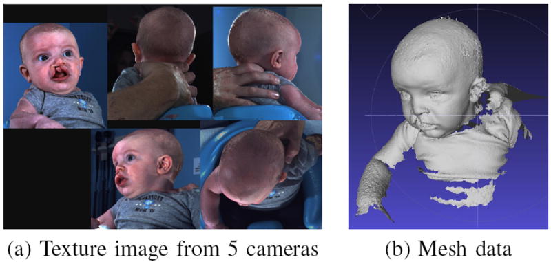
Raw data. (a) The texture image from 5 different cameras on left, right, front, back and top. (b) The 3D mesh composed of vertices and triangular connections.

There are three datasets in our study. One contains normal adults, with 21 scans from 10 individuals. The second one contains 64 meshes from 52 infants with unrepaired cleft lip. The last one consists of 35 meshes from 35 infants with repaired cleft lip. The latter two are extremely challenging, because these infants are too young to sit unsupported and need to be held by an adult or a positioning device. Although it is suggested that the subjects should face one of the cameras and have a relaxed expression when the scan is taken, the orientation and expression of infants are hard to control and the data can be very noisy.

III. Method

A. System Design

Our system is built for automatically cleaning the raw data and normalizing the 3D faces. With an input of 3D textured mesh data, our system first performs eye and nose region detection based on a machine learning technique and rotates the mesh so that the face is forward. Then, a face detection algorithm is used on the screenshot of the 3D mesh to detect the human face and a set of landmarks. After that, Procrustes alignment is applied to normalize the data so that a standard box can be used to cut the data uniformly. Last, some final cleaning methods are employed to further improve the data. Figure 2 illustrates the steps of our system.

Fig. 2.

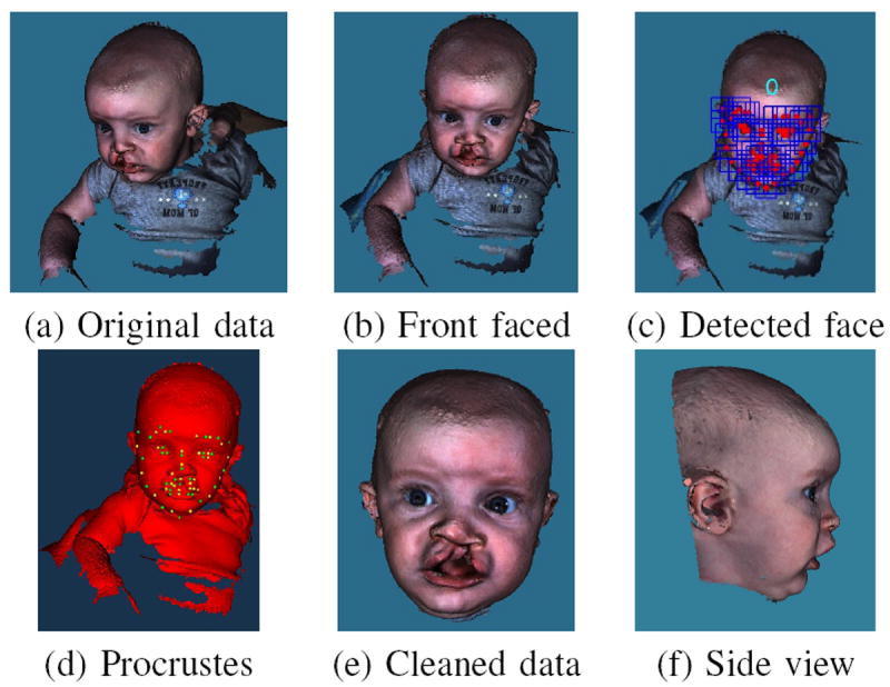
System design for automatically face extraction. (a) Original 3D mesh with texture. (b) Face rotated to a frontal position. (c) Face detected with 0 degree of rotation. (d) Procrustes aligned face with landmarks. (e) Front view of the cleaned data, the forehead and the front part of the skull are kept. (f) Side view of the cleaned data with the ears kept.

B. Eyes and Nose Tip Detection on Mesh

There are already some successful face recognition algorithms for 2D photos. In our dataset, the input contains both the reconstructed 3D mesh and 2D photos from several cameras. However, when capturing these photos, it is hard for the photographer to control the postures of the infants, so it is not guaranteed that one of the cameras will capture a good presentation of the face. Therefore, instead of applying a face recognition algorithm directly onto the photos taken by cameras, our first step is to ensure that the data is rotated to a suitable angle, so that the advantage of already existing and evaluated face recognition algorithms for 2D photos can be enhanced.

Our system uses three steps to rotate the 3D mesh and construct a frontal face screenshot for subsequent processes. The first step is to form a feature vector composed of a multiple-scale histogram of single-valued, low-level features. Next, two classifiers, one for inner eye corners and one for nose tip, are trained and the candidate points for eye and nose are selected. The third step is to select possible eye-nose triangle regions and rotate the data.

Our methodology starts by applying a low-level operator to every point on the surface mesh. The low-level features were first introduced for finding the symmetry plane of the face in [7] and are described here for convenience. The low-level operators extract local properties of the surface points by computing a single feature value υ_i for every point p_i on the mesh surface. In this work, shape index, curvedness and Besl-Jain curvature value are used for our experiments. Figure. 3 (a), (b) and (c) show examples of the shape index, curvedness and Besl-Jain curvature values of a 3D model, respectively.

Fig. 3.

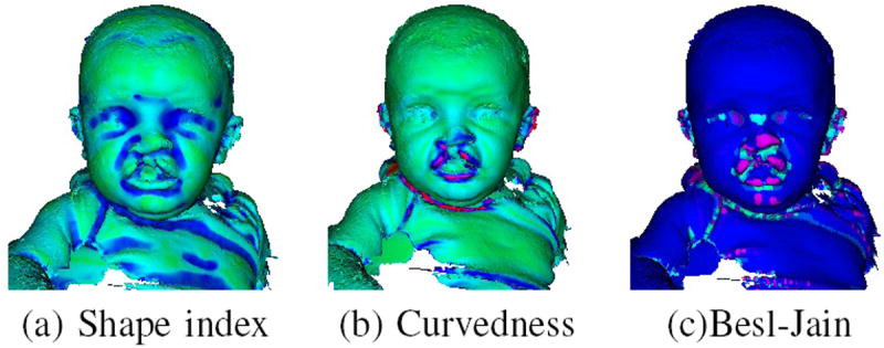
Local properties of the surface points. (a) The shape index of surface. Green means low and blue means high in shape index. (b) The curvedness of each point on one mesh. High curvedness is shown in red and low in green. (c) The Besl-Jain surface value on the surface. Blue means plane surface, dark purple means peak, light purple means pit, cyan means saddle ridge.

Next, instead of just using one value for a point p_i, a local histogram is used to aggregate the low-level feature values of each point. The histograms with multiple sizes of neighborhoods are combined together to form a large feature vector. Note that the three single-valued low-level features and the multiple scale histogram are all rotation invariant. This ensures that the eye and nose candidates can be selected despite the rotation of the original data.

After that, we chose to teach a classifier the characteristics of points that are the inner eye corner and nose tip because they are reliably detected. Histograms of low-level features were used to train a Support Vector Machine (SVM) classifier [8] to learn these three points on the 3D surface mesh. We used the SVM implemented in WEKA for our experiments [9]. The training data for supervised learning for the classifiers was obtained by manually marking eye and nose points on the surface of each training object. The histogram of low-level features of each of the marked points was saved and used for the training.

A small training set, consisting of 40 head meshes was used to train the classifier to learn the characteristics of the eye or nose points in terms of the histograms of their low-level features. After training is complete, the classifier is able to label each of the points of any 3D object as either inner eye corner or nose or neither and provides a confidence score for its decision. A threshold T is applied to the confidence scores for the inner eye conner or nose tip. In our experiments, we used T = 0.98 to keep only the points with high confidence scores from the classifiers.

Although the classifiers for eye and nose were very powerful, there were still false positive regions in the predicted results. We developed a systematic way to find the eye-nose-eye triangle area. First, the candidate points from both classifiers are grouped to form regions. Second, small regions (< 50 points) are removed. Third, a pair of eye regions that have a similar number of points, along with a nose region that lies almost equidistant from those two eye regions are picked. Last, some geometric thresholds are used to rule out regions that are too small or too big.

After the eye-nose-eye region is determined, the head is rotated so that the eye regions are leveled and symmetric and the nose appears to be right underneath the eye center. This produced a frontal face screenshot for the subsequent steps.

C. 2D Face Detection

The problem of finding and analyzing faces from 2D images is a foundational task in computer vision and there are multiple existing techniques. In Zhu’s work [10], the tasks of face detection, pose estimation and landmark estimation are jointly addressed by a model based on a mixture of trees with a shared pool of parts. Every facial landmark is modeled as a part and global mixtures are used to capture topological changes. This method is applied to our data after the face is rotated to a frontal position. The results after this step include: face location, head pose estimation, and landmarks on the 2D screenshot. Figure 4 illustrates why the previous rotation step is essential. Because the babies’ pose and expression are very hard to control, if the face detection method is applied directly to the original photo without pose normalization, it sometimes leads to a failure in face detection or even a false positive result. After pose normalization, when there is a clear frontal face in the image, the task is much easier for both face detection and landmark localization algorithm.

Fig. 4.

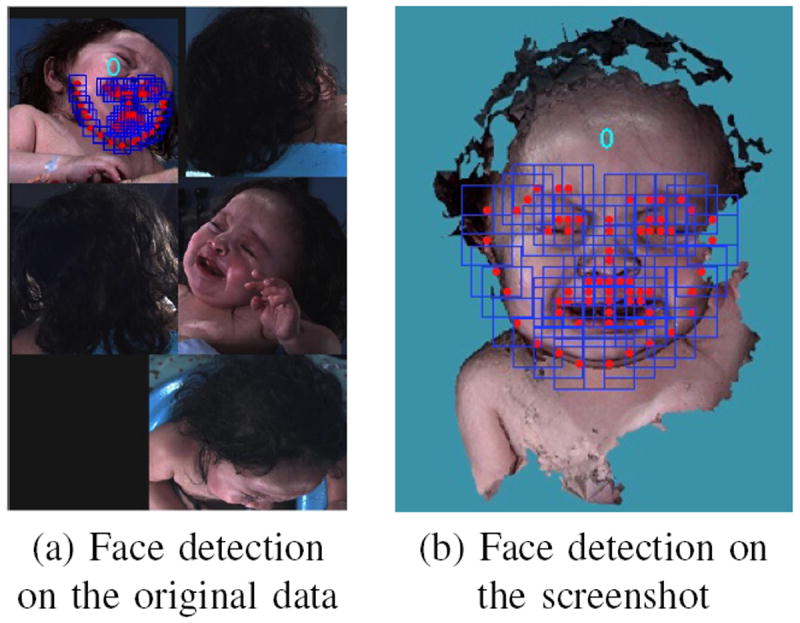
Same face detection algorithm applied to original data and screenshot after face rotation. The number 0 appears on the image means frontal face position. (a) shows the pose estimation is not true and the landmarks are not properly located if the face detection algorithm is applied directly to the original photo. (b) returns a true positive result, with a detection of frontal face.

D. Face Normalization

Once the frontal face is detected, the 3D landmarks are calculated by projecting the extracted 2D landmarks on the screenshot from the previous step. The 3D mesh faces are then normalized by Procrustes analysis (PA) [11]. In this step, a random head mesh D_m with landmarks L_m is selected as the approximate mean shape. Then every head mesh D_j with landmarks L_j is aligned to the approximate mean shape by translation, scaling and rotation so that the sum of squared errors of the landmarks L_j and L_m is minimized. Then a new mean shape D_m with landmarks L_m is calculated based on the average of the aligned data. The steps are iterative until the mean shape is stable and each head mesh is aligned to the mean.

Figure 5 shows the experimental data of landmarks before and after Procrustes analysis. The red dots represent the landmarks L_m. Before Procrustes analysis, the green dots in Fig 5 (a) are all scattered, while the blue dots in Fig 5 (b) shows the landmarks after the Procrustes analysis gathered around the mean landmarks L_m.

Fig. 5.

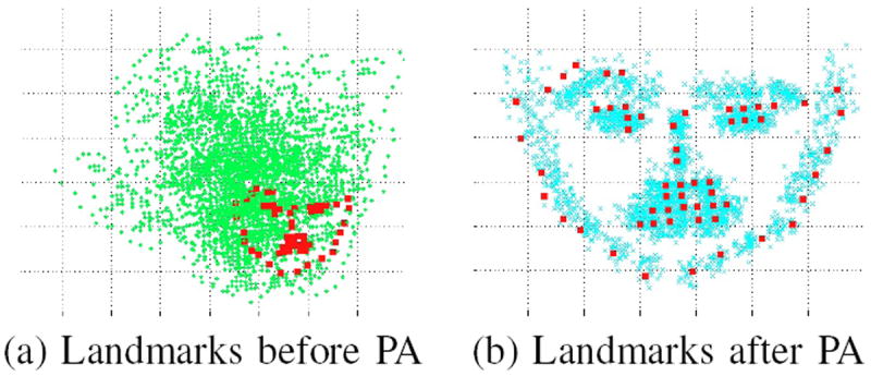
Landmarks before and after procrustes analysis.

E. Final Cleanup

Because all the data are normalized to the same scale and rotation, a standard bounding box is used to cut the data and meet the requirements for keeping the ears and forehead area, as shown in Fig. 6(a). For an adult, this standard bounding box is adequate to separate the face from other parts because adults tend to have a long neck. However, for children especially young babies, there is still clothing or other noise under the chin area due to the shortness of their necks. Some additional cleanup steps, including surface normal thresholding and color thresholding, are used to remove this noise. For every point in the bounding box p_i, the surface normal vector is calculated, with N x_i, N y_i and N z_i as the normal vector projection in x, y and z axis respectively. The larger N y_i is, the more the surface around point p_i is facing up. Figure 6 (c) shows the normal value in the y direction. Considering the points around the lower jaw and chin are all facing downward and the points in the clothing and shoulders are facing up, a threshold T_N y is used to differentiate the shoulder and chest from the face. Another threshold is used in color space. The colors of the points are converted from RGB space to HSV space; the hue values for every point in the bounding box are illustrated in Fig. 6 (d). The average hue value for the cheek area is calculated. Any point with a large difference from the average hue value in the cheek area is removed. Figure 6(b) shows that after these two cleanup steps, the clothing and noise under the chin are all removed.

Fig. 6.

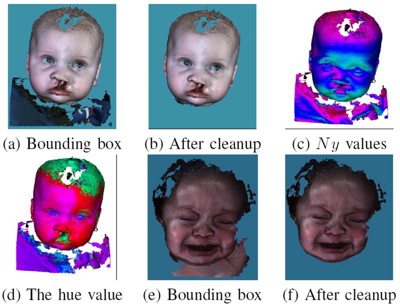
Final cleanup. (a) Cut by a standard boundary box. (b) Cleaned by using normal and color thresholds. (c) The surface normal value in the y direction, red means the surface normal is pointing up, and green means facing down. (d) The hue value for the face. A thresholds was chosen for cleaning the noise underneath the chin. (e) (f) Another example before and after final cleanup.

IV. Experiments and Results

For our experiments, we use the WEKA [9] implementation of the SVM classifier in the eye and nose detection step. This step is considered accurate when the eye-nose triangle is detected correctly and the face is rotated to a frontal position. This step achieves 100% accuracy in the normal dataset, 94% in the unrepaired cleft dataset and 97% in the repaired cleft dataset. For the images in which the classifier failed in detecting eye-nose regions, the face is rotated manually to face forward for latter processes.

The software provided by Zhu [10] was used for face detection on the screenshot produced by the previous step. This algorithm is extremely successful when the input is a frontal face, achieving 100% in the face detection task with all three datasets. After Procrustes analysis and normalizing all the detected faces, the standard box successfully keeps the face, forehead, front part of the skull and ears for all the data from normal, unrepaired and repaired cleft lip data.

In the last step of removing the clothes, chest and shoulder areas under the chin, in order to avoid over cropping, we chose the threshold to be very relaxed to ensure that the chin is well maintained. We found there are 6% and 9% with very small amount of clothes or skin in the chest remaining underneath the chin for babies with cleft lip in the datasets before and after surgery, respectively, as show in Table I.

TABLE I.

Accuracy for Each Step in the Process

Dataset	normal	unrepaired cleft	repaired cleft
number of instances	21	64	35
eyes and nose detection	21 (100%)	60 (94%)	34 (97%)
face detection	21 (100%)	64 (100%)	35 (100%)
ear and forehead	21 (100%)	64 (100%)	35 (100%)
no clothes left	21 (100%)	60 (94%)	32 (91%)

V. Conclusion

This paper introduces a system to crop out the face from 3D textured mesh data in infants as young as 3 months old and in adults to meet the requirements of medical researchers. The system takes a 3D mesh, detects the inner eye corners and the nose tip, rotates the data and saves a screenshot. Then the screenshot is analyzed by a 2D face detection and landmark estimation algorithm. After the landmarks are obtained, the data are normalized, allowing for a standard boundary crop. Finally, the surface normal and color are used to threshold some noise underneath the chin area. The results on normal and challenging patient datasets show that the whole process is very reliable. It detects the face and maintains the face area, the forehead, the ears and the front part of the skull with a 100% rate of success.

References

- 1.Hammond P, Forster-Gibson C, Chudley AE, Allanson JE, Hutton TJ, Farrell SA, McKenzie J, Holden JJA, Lewis MES. Face–brain asymmetry in autism spectrum disorders. Molecular psychiatry. 2008;13(6):614–623. doi: 10.1038/mp.2008.18. [DOI] [PubMed] [Google Scholar]
- 2.Atmosukarto I, Shapiro LG, Starr JR, Heike CL, Collett B, Cunningham ML, Speltz ML. Three-dimensional head shape quantification for infants with and without deformational plagiocephaly. The Cleft Palate-Craniofacial Journal. 2010;47(4):368–377. doi: 10.1597/09-059.1. [DOI] [PMC free article] [PubMed] [Google Scholar]
- 3.Wilamowska K, Shapiro L, Heike CL. Classification of 3D face shape in 22q11. 2 deletion syndrome. Biomedical Imaging: From Nano to Macro, 2009. ISBI’09. IEEE International Symposium on; IEEE; 2009. pp. 534–537. [Google Scholar]
- 4.Wu J, Tse R, Shapiro LG. Learning to rank the severity of unrepaired cleft lip nasal deformity on 3d mesh data. International Conference in Patten Recognition(ICPR), 2014 IEEE Conference on; IEEE; 2014. [DOI] [PMC free article] [PubMed] [Google Scholar]
- 5.3dMD. http://www.3dmd.com.
- 6.Mian AS, Bennamoun M, Owens RA. Automatic 3d face detection, normalization and recognition. 3DPVT. 2006;6:735–742. [Google Scholar]
- 7.Wu J, Tse R, Heike CL, Shapiro LG. Learning to compute the symmetry plane for human faces. ACM Conference on Bioinformatics, Computational Biology and Health Informatics; ACM; 2011. [Google Scholar]
- 8.Suykens J, Vandewalle J. Least squares support vector machine classifiers. Neural processing letters. 1999;9(3):293–300. [Google Scholar]
- 9.Hall M, Frank E, Holmes G, Pfahringer B, Reutemann P, Witten LH. The weka data mining software: an update. ACM SIGKDD Explorations Newsletter. 2009;11(1):10–18. [Google Scholar]
- 10.Zhu X, Ramanan D. Face detection, pose estimation, and landmark localization in the wild. Computer Vision and Pattern Recognition (CVPR), 2012 IEEE Conference on; IEEE; 2012. pp. 2879–2886. [Google Scholar]
- 11.Gower JC. Generalized procrustes analysis. Psychometrika. 1975;40(1):33–51. [Google Scholar]