Substitution and pooling in visual crowding induced by similar and dissimilar distractors

Abstract

Visual crowding refers to a phenomenon whereby objects that appear in the periphery of the visual field are more difficult to identify when embedded within clutter. Pooling models assert that crowding results from an obligatory averaging or other combination of target and distractor features that occurs prior to awareness. One well-known manifestation of pooling is feature averaging, with which the features of target and nontarget stimuli are combined at an early stage of visual processing. Conversely, substitution models assert that crowding results from binding a target and nearby distractors to incorrect spatial locations. Recent evidence suggests that substitution predominates when target–flanker feature similarity is low, but it is unclear whether averaging or substitution best explains crowding when similarity is high. Here, we examined participants' orientation report errors for targets crowded by similar or dissimilar flankers. In two experiments, we found evidence inconsistent with feature averaging regardless of target–flanker similarity. However, the observed data could be accommodated by a probabilistic substitution model in which participants occasionally “swap” a target for a distractor. Thus, we conclude that—at least for the displays used here—crowding likely results from a probabilistic substitution of targets and distractors, regardless of target–distractor feature similarity.

Introduction

Objects that appear in the periphery of the visual field are more difficult to identify when surrounded by clutter. This phenomenon—known as visual crowding (Bouma, 1970; Strasburger, Harvey, & Rentschler, 1991; see also earlier work by Ehlers, 1936; Stuart & Burian, 1962)—places important constraints on many everyday visual tasks, including reading (e.g., Chung, 2002; Pelli et al., 2007), visual search (Carrasco, Evert, Chang, & Katz, 1995; Vlaskamp & Hooge, 2006), and object recognition (Levi, 2008; Pelli, 2008).

Pooling models propose that crowding results from an obligatory combination of target and flanker features at a relatively early stage of visual processing (prior to the point at which features or objects can be consciously accessed or reported; e.g., Balas, Nakano, & Rosenholtz, 2009; Dakin, Cass, Greenwood, & Bex, 2010; Greenwood, Bex, & Dakin, 2009; Parkes, Lund, Angelucci, Solomon, & Morgan, 2001; van den Berg, Roerdink, & Cornelissen, 2010). Pooling can take many forms, including (but not limited to) feature averaging (e.g., Parkes et al., 2001), positional averaging (e.g., Dakin et al., 2010; Greenwood et al., 2009), and pixel averaging or blurring. More complicated forms of pooling based on local first-, second-, and third-order statistics are also plausible (e.g., Balas et al., 2009; Freeman & Simoncelli, 2011). Each alternative is assumed to result in a percept that preserves the ensemble statistics of the display but lacks information about local features or stimuli.

Here, we focus on feature averaging and ask whether it suffices to explain reductions in orientation acuity within displays containing a set of oriented stimuli. In a relevant study, Parkes et al. (2001) asked participants to report the tilt of a Gabor surrounded by an array of horizontal distractors and found that tilt thresholds (i.e., the minimum target tilt needed to perform the task with criterion accuracy) decreased monotonically as the number of tilted distractors decreased. In a second experiment, the authors asked participants to report the configuration of three tilted Gabors presented among horizontal distractors. Performance on this latter task was at chance levels, suggesting that even though the number of tilted distractors had a large effect on tilt thresholds participants were unable to identify or report the identity of any single Gabor. These results suggest that under some circumstances (e.g., for displays containing simple oriented stimuli) crowding results from an obligatory averaging of target and distractor features. However, these findings can also be accommodated by a probabilistic substitution model in which participants occasionally mistake or “swap” the target Gabor with a distractor. Indeed, in a recent paper (Ester, Klee, & Awh, 2014), we asked participants to report the precise orientation of a crowded or uncrowded target and fit the resulting distributions of response errors (i.e., reported minus actual target orientations) with quantitative functions that assume feature averaging or probabilistic substitution (in which participants occasionally confuse a distractor orientation with the target orientation and report the former). In all cases, the observed data were well described by a function assuming substitution and poorly described by a function assuming orientation averaging.

One limitation of this study was that the distractors used to induce crowding were quite dissimilar from the target (e.g., tilted ±60°, ±90°, or ±120° relative to the target), and there is reason to suspect that different forms of crowding may predominate when target–distractor similarity is high. For example, recent reports suggest that different kinds of target–distractor interference appear to manifest themselves when similarity is high versus low (“repulsion” vs. “assimilation,” respectively; see Mareschal, Morgan, & Solomon, 2010). Thus, one possibility is that feature averaging predominates when target–distractor similarity is high, and substitution predominates when similarity is low. The goal of this study was to evaluate this possibility.

Experiment 1

Following Ester et al. (2014), we asked participants to report the orientation of a crowded or uncrowded target. When present, crowders were tilted ±15°, ±30°, ±60°, or ±90° relative to the target with an equal number of crowders tilted clockwise and counterclockwise. For each participant and experimental condition, we generated a distribution of response errors (i.e., reported minus actual target orientation), which were then fit with quantitative models that assume feature averaging or probabilistic substitution. We then compared these models to determine which provided a better description of the data.

Methods

Participants

Twenty-two undergraduate students from the University of California, San Diego, completed a single 1.5-hr testing session in exchange for course credit. All participants reported normal or corrected-to-normal visual acuity. Data from one participant were subsequently discarded due to exceptionally poor performance (specifically, s/he appeared to be responding randomly, and we could not extract stable estimates for either the averaging or substitution models as a result); the data reported here reflect the remaining 21 participants. All experimental procedures were approved by the local institutional review board, and all participants gave both written and oral informed consent in accordance with the Declaration of Helsinki.

Stimuli and display

Stimuli were generated in Matlab (Version 2010b; Natick, MA) and rendered on a 19-in. CRT monitor cycling at 60 Hz (resolution 800 × 600) via Psychophysics Toolbox software (Version 3.1.1; Brainard, 1997; Pelli, 1997). Participants were seated in a dimly lit room approximately 60 cm from the display (head position was unconstrained). From this distance, targets and crowders subtended 2.67° and appeared ±9.23° from fixation along the horizontal meridian. The center-to-center distance between adjacent stimuli was fixed at 3.33°.

Procedure

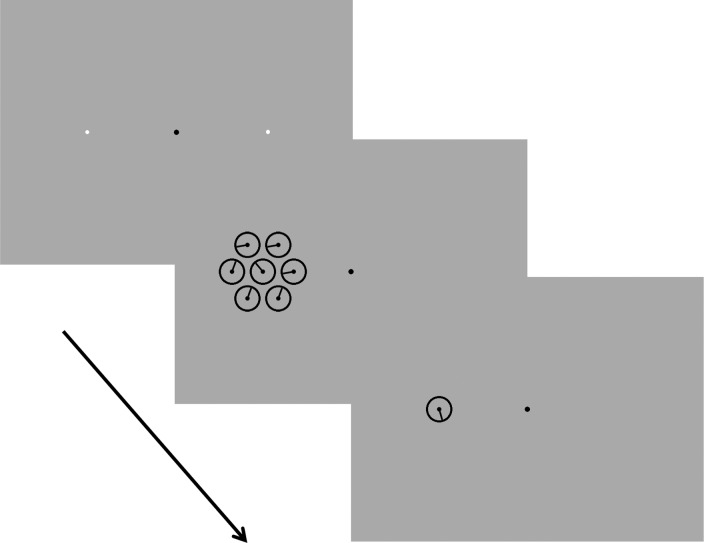
A schematic of the task is shown in Figure 1. Each trial began with the presentation of a fixation display containing a small black dot (subtending 0.25°) and two small (0.18°) white “placeholders” at ±9.23° eccentricity along the horizontal meridian. After a short interval (determined on a trial-by-trial basis by sampling from a uniform distribution with a range of 400–700 ms), a target display was presented for 75 ms. In 50% of trials, a single, randomly oriented “clock face” (the target) was rendered over one of the two placeholders (“uncrowded” trials). In the remaining 50% of trials, the target was embedded within six additional distractors (“crowded” trials; see Figure 1). When present, three randomly chosen distractors were tilted ±15°, ±30°, ±60°, or ±90° clockwise from the target, and the remaining distractors were tilted counterclockwise by an equal amount. Participants were instructed to ignore the distractors and remember the orientation of the target that appeared over the placeholder. After a 400-ms blank interval, a randomly oriented probe was presented at the same location as the target, and participants used the arrow keys on a standard keyboard to adjust the orientation of the probe until it matched their percept of the target (pressing the spacebar to enter their final response). Participants were instructed to respond as precisely as possible, and no response deadline was imposed. Trials were separated by a 250- to 600-ms interval (randomly chosen in each trial). Each participant completed 13 (n = 1), 14 (n = 2), or 16 (n = 18) blocks of 64 trials for a total of 832, 896, or 1024 trials, respectively.

Figure 1.

Behavioral task used in Experiment 1. Each trial began with the presentation of a fixation display (upper panel) for a short interval. A target display (middle panel) was presented for 75 ms, and participants were instructed to identify the orientation of the stimulus that appeared over the small white cue in the fixation display. When present, a randomly chosen subset of flankers were rotated 15°, 30°, 60°, or 90° clockwise relative to the target, and the remaining three were rotated counterclockwise by an equivalent amount. After a short blank interval, a randomly oriented probe appeared at the target location; participants adjusted its orientation to match their memory of the target (displays are not drawn to scale; see Methods for further information on specific display parameters).

Model fitting and model comparison

We fit each participant's response errors (i.e., reported minus actual target orientation) within each condition with quantitative functions that assume either feature averaging or probabilistic substitution. During uncrowded trials, performance is well described by a “mixture model” that combines a von Mises distribution (a circular variant of the standard normal distribution) with mean μ and concentration k with a uniform distribution with height ρ:

where x is a vector of response errors in radians with range [−π, π]. I₀ is the modified Bessel function of the first kind of order 0:

In Equation 1, μ (in radians) and k (dimensionless units) correspond to the mean (center) and concentration of the von Mises distribution (respectively), and ρ determines the height of a uniform distribution over the range (−π, π]. Concentration is a reciprocal measure of dispersion, and as k increases, the von Mises begins to approximate a normal distribution with mean μ and variance 1/k (Abramowitz & Stegun, 1964; Fisher, 1993). Thus, we defined a measure of response variability as σ = √k − 1 with units in radians. Estimates of μ and σ were then converted to degrees by multiplying these values by (180/π).

Equation 1 can also be used to quantify performance in crowded trials given a simple linear feature averaging model (e.g., Parkes et al., 2001). Consider a scenario in which the target is surrounded by three distractors tilted 30° clockwise to the target and three distractors tilted 30° counterclockwise to the target. If the target and flankers are averaged prior to reaching awareness, then the clockwise and counterclockwise distractors' features should cancel, and the precision of participants' responses (quantified by σ) should equal the precision of responses in the uncrowded condition (alternately, if the target and each distractor contributes an independent (noisy) orientation signal, then averaging could actually improve the precision of participants' responses). Conversely, any decrease in estimates of k (corresponding to a “broader” distribution of report errors and thus, lower precision) is inconsistent with feature averaging.

Of course, other averaging rules are plausible. For example, perhaps flankers further away from or closer to fixation are weighted more heavily during averaging process (see, e.g., Chastain, 1982; Strasburger & Malania, 2013, for examples of instances in which “inner” and “outer” flankers have an asymmetric influence on alphanumeric character recognition performance under various circumstances). In the current study, this would produce a systematic shift in μ toward the pooled orientations of the distractors nearest to or furthest from fixation.

To quantify response errors under the assumption that crowding results from probabilistic substitution (in which distractors are occasionally “swapped” with the target), we fit each participant's distribution of errors with a trimodal function:

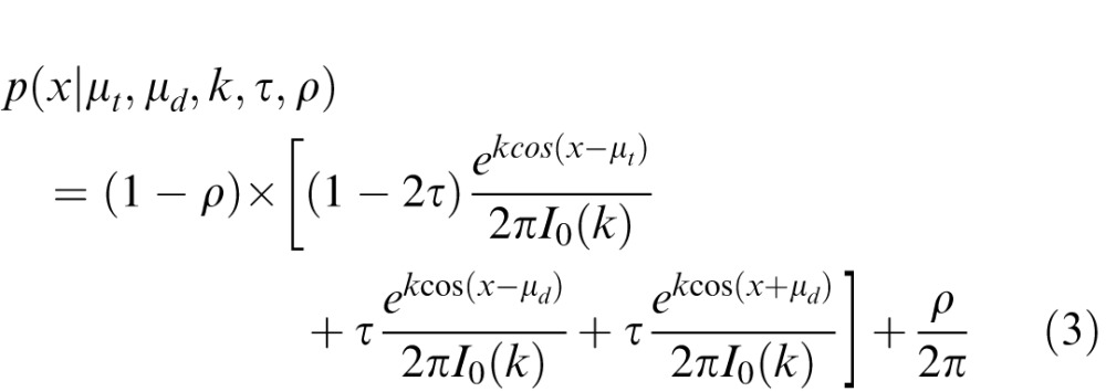where τ corresponds to the probability of reporting a distractor orientation; μ_t corresponds to the target orientation, and μ_d corresponds to absolute distractor orientation relative to the target (i.e., 15°, 30°, 60°, or 90°); k and ρ are as defined above. A trimodal distribution was used to account for the fact that in a given trial participants could report the orientation of the target, a counterclockwise flanker, or a clockwise flanker. For convenience, we assumed that targets and distractors would be reported with the same precision (σ; estimated from k using the method described above), and we fixed both μ_t and μ_d at the target and flanker orientations, respectively, during fitting.

We used Bayesian model comparison (BMC; MacKay, 2003; van den Berg, Shin, Chou, George, & Ma, 2012; Wasserman, 2000) to compare the averaging and substitution models for each crowded condition. BMC returns the likelihood of a model given the observed data and includes a penalty for model complexity. Additionally, BMC integrates information over parameter space and thus accounts for variability in model performance over a range of possible parameter values. Each model m from the set of models M (in our case, the pooling and substitution models) produces an error distribution p(D; m, Ω), where D is a vector of report errors, and Ω is a vector of j model parameters. For each model, we calculate the probability of finding D under this distribution, averaged over free parameters:

For numerical convenience, we take the logarithm and rewrite Equation 4 as

where log L(M; Ω) = and L_max(M) = max L(M; Ω). Semicolons denote operations applied to the entire set of models M (i.e., m₁, m₂ … m_n). Subtracting L_max(M) avoids numerical problems by ensuring that the exponential in the integrand is of order 1 near the maximum likelihood value of Ω.

For simplicity, we set the prior of the jth model parameter, i.e., p(Ω_j|M), to be uniform over interval R_j (see Table 1). That is, we iteratively computed the log likelihood of each model using all possible combinations of parameter values over the range R_j (min) to R_j (max) and selected the set of parameter values that maximized this quantity. Equation 5 thus becomes

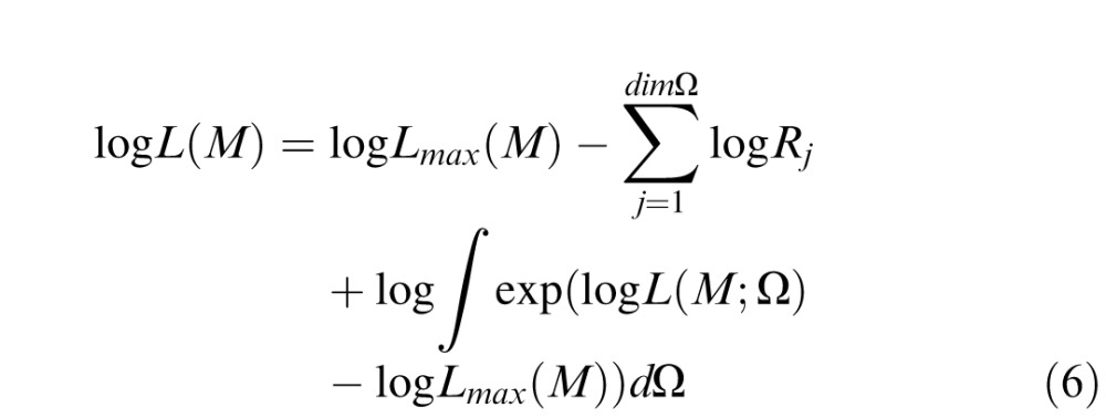Table 1.

Ranges of parameter values used in BMC. Notes: An exhaustive grid search was used to find the combination of parameters that maximized the log likelihood of the pooling and substitution models. Units of μ and are in radians, and units of k are dimensionless.

	μ	k	τ	ρ
Lower bound	−π/3	3	0	0
Upper bound	π/3	40	0.9	0.9
Increment	0.01	0.1	0.01	0.01

Statistical analyses

We report traditional p values as well as Bayes factors throughout the paper. Unlike traditional null-hypothesis significance testing, Bayesian analyses allow one to incorporate prior knowledge about the likely state of the world and to make precise statements about the likelihood of a hypothesis, including the null, given the observed data. Consider the following hypothetical scenario: We wish to compare a null model M₀ with an alternative model M₁. M₀ states that the true magnitude of the difference between two conditions is 0 whereas M₁ states that the true magnitude of the difference is nonzero, and our a priori uncertainty about the true magnitude of the effect is a normal distribution over a plausible range of possible effect sizes. The a priori plausibility of model M₁ to M₀ is given by p(M₁)/p(M₀). Given this ratio and the observed data, Bayes rule allows one to calculate the posterior odds of each model given the data:

The ratio p(D|M₁)/p(D|M₀) is called the Bayes factor (bf), and it describes the amount by which the data have changed the prior odds. For example, a bf of 10 indicates a 10-to-1 change in the prior odds favoring the alternative model. Conversely, a bf of 0.1 indicates a 10-to-1 change in the prior odds favoring the null model (see Edwards, Lindman, & Savage, 1963, and Kass & Raftery, 1995, for further information).

Bayesian analyses were performed in R using the “BayesFactor” package developed by Richard Morey and Jeffrey Rouder (available for download at bayesfactorpcl.r-forge.r-project.org).

Results

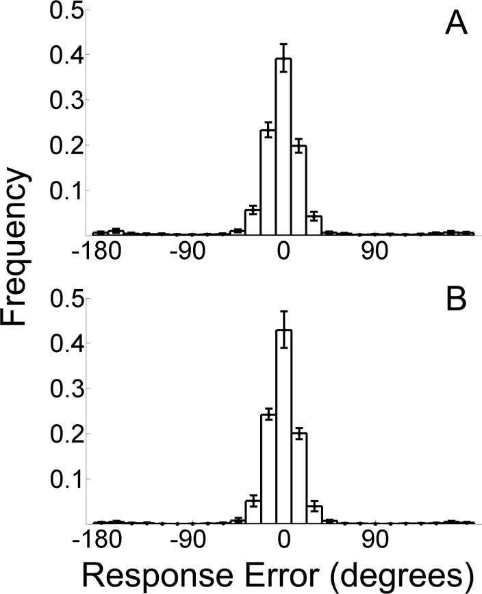
Figure 2A depicts the mean distribution of response errors during uncrowded trials. As expected, response errors were tightly distributed around the target orientation (i.e., 0° response error) with approximately 8% of responses attributable to random guessing (Figure 2B is discussed in Experiment 2 below).

Figure 2.

Histograms of response errors for uncrowded displays in Experiments 1 (A) and 2 (B). Error bars are 95% confidence intervals.

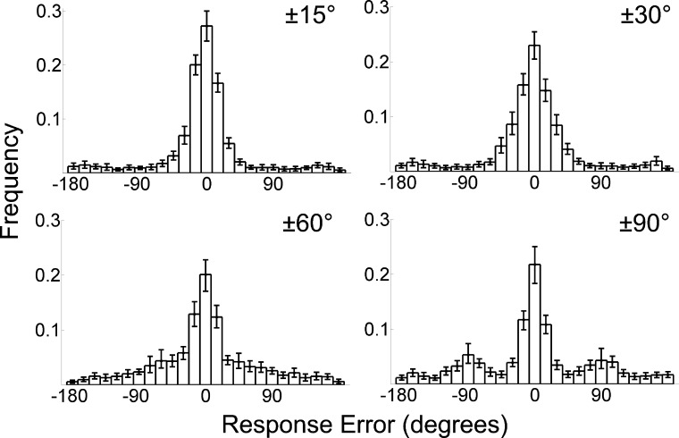
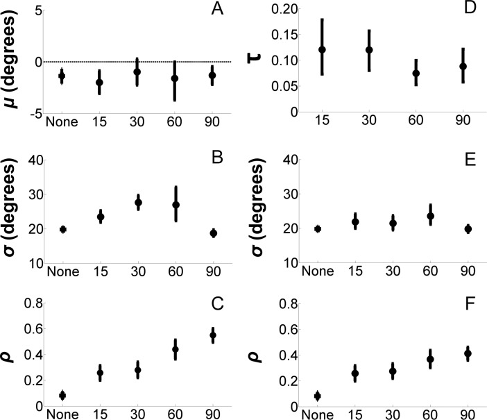
Next, we fit each participant's response errors within each crowded condition with the averaging and substitution models described in Equations 1 and 2. Histograms of response errors within each crowded condition are shown in Figure 3, and the parameters for the best-fitting averaging and substitution models are shown in Figure 4. BMC was used to compare the performance of the two models within each crowded condition. Specifically, we computed log likelihoods for each model over a large range of possible parameter values (see Table 1) and extracted the parameter estimates that maximized this quantity (separately for each condition). We then averaged the log likelihoods of both models within each condition across participants and subtracted the averaged log likelihood of the averaging model from the averaged log likelihood of the substitution model. In this formulation, a log likelihood difference of x means that the data are x times more likely under the substitution model than the averaging model.

Figure 3.

Response errors during crowded trials in Experiment 1. Error bars are 95% confidence intervals.

Figure 4.

Parameters of the best fitting pooling (left column) and substitution (right column) models. (A, B, and C) Estimates of μ, σ, and ρ estimated from the pooling model (Equation 1) as a function of distractor presence and target–distractor rotation differences (±15° through ±90°). (D, E, and F) Estimates of τ, σ, and ρ obtained from the substitution model in Equation 2 as a function of distractor presence and target–distractor differences. By definition, τ = 0 when there are no distractors in this display, so this condition has been omitted from (D). The estimate of σ for uncrowded trials in (E) was obtained via the pooling model, i.e., it is identical to the estimate shown in (C). Error bars are 95% confidence intervals.

For the ±15°, ±30°, and ±60° conditions, the substitution model marginally outperformed the pooling model. Specifically, averaged log likelihoods were 0.80, 1.33, and 1.48 units higher for the substitution relative to the pooling model for three conditions, respectively. These correspond to approximately 2.22-, 3.78-, and 4.40-to-1 odds favoring the substitution model over the pooling model. However, the substitution model outperformed the averaging model within the ±90° condition by a substantial amount. Specifically, the averaged log likelihood of the substitution model was 3.56 units larger than the averaged log likelihood of the averaging model; this corresponds to approximately 35-to-1 odds favoring substitution over averaging. These results suggest that crowding induced by more dissimilar flankers (e.g., ±60°, ±90°) results from a probabilistic substitution of targets, consistent with earlier work (Ester et al., 2014). However, they are somewhat ambiguous with respect to the effect of similar flankers (±15° or ±30°).

Next, we examined the plausibility of the averaging model using two similar-flanker conditions (±15° and ±30°; qualitatively identical results were obtained when we also included the ±60° condition) by comparing estimates of μ, σ, and ρ during crowded and uncrowded trials. These are shown in Table 2. Recall that in each crowded trial three distractors were tilted clockwise relative to the target in each trial while the remainder were tilted counterclockwise. If the orientations of the targets and distractors are pooled (averaged) at an early stage of processing (e.g., Parkes et al., 2001), then the effect of the distractors should cancel, and performance should equal levels observed in the uncrowded condition. To evaluate this possibility, estimates of μ, σ, and ρ returned by the averaging model were subjected to separate one-way ANOVAs with condition (uncrowded, ±15°, ±30°) as the sole within-subjects factor. This analysis revealed a significant effect of condition on σ (p = 2.84e − 08, bf = 2.90e + 06; Figure 4C) and on ρ (p < 2.19e − 11, bf = 3.22e + 08; Figure 4E), but not on μ (p = 0.27, bf = 0.36; Figure 4A). Post hoc comparisons (repeated measures t tests) revealed robust differences between estimates of σ for the uncrowded and ±15° conditions (p = 0.002, bf = 19.00), and the uncrowded and ±30° conditions (p = 1.39e − 06, bf = 13,256). Estimates of σ were also significantly different across the ±15° and ±30° conditions (p = 0.003, bf = 103). Identical comparisons on ρ revealed robust differences between the uncrowded and ±15° conditions (p = 4.80e − 08, bf = 2.94e + 05), and the uncrowded and ±30° conditions (p = 1.56e − 07, bf = 9.91e + 04). The difference between the ±15° and ±30° conditions was not significant (p = 0.29, bf = 0.38).

Table 2.

Estimates of k and τ returned by the pooling model in Experiment 1 for the no-flanker and similar-flanker (±15° and ±30°) conditions. Notes: Values of μ and σ are in degrees. Values in brackets are 95% confidence intervals.

	μ	σ	ρ
No flankers	−1.37 [−3.60– −2.37]	19.78 [16.58–22.90]	0.08 [0.05–0.12]
±15°	−2.00 [−3.09– −0.91]	23.45 [21.73–25.30]	0.26 [0.20–0.32]
±30°	−0.97 [−2.29–0.40]	27.63 [25.48–19.77]	0.28 [0.22–0.34]

These results are inconsistent with simple averaging models in which target and distractor values are averaged prior to reaching awareness (e.g., Parkes et al., 2001). Under such a model, one would expect roughly equivalent performance during crowded and uncrowded conditions because the influence of clockwise and counterclockwise distractors should cancel during the averaging operation. However, more complex averages are also plausible. For example, perhaps distractors nearer the fovea are weighted more heavily during the averaging process. This alternative is motivated by observations suggesting that “inner” or “outer” flankers may have a greater effect on recognition performance under certain conditions (e.g., Strasburger, Rentschler, & Juttner, 2011; Strasburger & Malania, 2013). Here, one would expect estimates of μ to be systematically shifted away from 0 and toward the mean of the three distractors nearest or furthest from fixation in each trial. To evaluate this possibility, we conducted separate analyses in which we extracted the orientations of the three distractors either nearest or furthest from fixation in each ±15° and ±30° trial. We then sorted each participant's report errors into one of two bins, depending on whether the mean orientation of the flankers were tilted counterclockwise or clockwise relative to the target (data were pooled across ±15° and ±30° trials to ensure adequate statistical power). We then estimated μ within each bin using Equation 1. False-discovery-rate-corrected repeated-measures t tests revealed no effect of mean distractor rotation direction (i.e., clockwise or counterclockwise relative to the target) on μ, σ, or ρ; both ps > 0.70 and both bfs < 0.27. Qualitatively similar results were obtained when we included all target–distractor tilts in this analysis.

Thus far, our findings are inconsistent with a feature-averaging model of crowding either because a substitution model provides a better description of the observed data (e.g., in the ±60° and ±90° conditions) or because the averaging model actually behaves in a manner inconsistent with feature averaging (e.g., across the uncrowded, ±15° and ±30° conditions). Thus, we next consider an alternative model. Under this model, the observed distributions of response errors are a sum of three underlying distributions: one centered at the target's orientation, and one centered at each distractor orientation (e.g., ±15°). Unfortunately, it is difficult to unambiguously recover these three subdistributions (see below). Nevertheless, given that this model provided a reasonable description of the observed data (average r² across participants and crowded conditions was 0.77; Figure 3C, D), we decided to examine the behavior of this model across the various crowded conditions. Estimates of σ, τ, and ρ for each crowded condition (i.e., ±15° through ±90°) were subjected to a one-way ANOVA with target–flanker rotation as the sole within-subjects factor. These analyses revealed a significant effect of rotation on ρ (p < 2.47e − 07, bf = 5.48e + 04; Figure 4F), but no effect of rotation on either σ (p = 0.21, bf = 0.42; Figure 4D), or τ (p = 0.24, bf = 0.36; Figure 4B).¹ Inspection of Figure 3 suggests that increasing target–distractor rotations increased the likelihood of random responses but has no discernable effect on the likelihood of reporting a nontarget or the precision of participants' responses.

As mentioned above, we were unable to recover unambiguously trimodal distributions in the ±15°, ±30°, and ±60° conditions. The reason for this is that it is extremely difficult to disambiguate proximal target and distractor error distributions, particularly when the distance between the target and distractors is less than or equal to the precision with which a participant can encode and report information. To illustrate this, we generated a set of trimodal response distributions using parameters returned by the substitution model during ±15°, ±30°, and ±60° trials. We then generated 100,000 samples from each distribution and compared how well the averaging and substitution models in Equations 1 and 2 were able to characterize the data. In nearly all cases, the two models performed equivalently even though the data were synthesized from a trimodal distribution. Thus, in our view, the fact that the simple averaging model equals or outperforms the substitution model when target–distractor similarity is high (±15° and ±30°) constitutes only weak support for feature averaging.

Experiment 2

Experiment 2 was similar to Experiment 1 with two exceptions. First, we eliminated the ±30° and ±90° target–distractor tilt conditions. Second, we systematically varied the center-to-center distance between the target and distractors. It is well known that increasing the distance between a target and nearby distractors reduces the severity of crowding (e.g., Bouma, 1970; Scolari, Kohnen, Barton, & Awh, 2007). This allowed us to examine whether the frequencies of distractor and random responses were modulated by a factor known to determine crowding strength.

Method

Participants

Eighteen additional undergraduate students from UCSD completed a single 1.5-hr testing session in exchange for course credit. All participants gave both written and oral informed consent and reported normal or corrected-to-normal visual acuity. All experimental procedures were approved by the local institutional review board.

Procedure

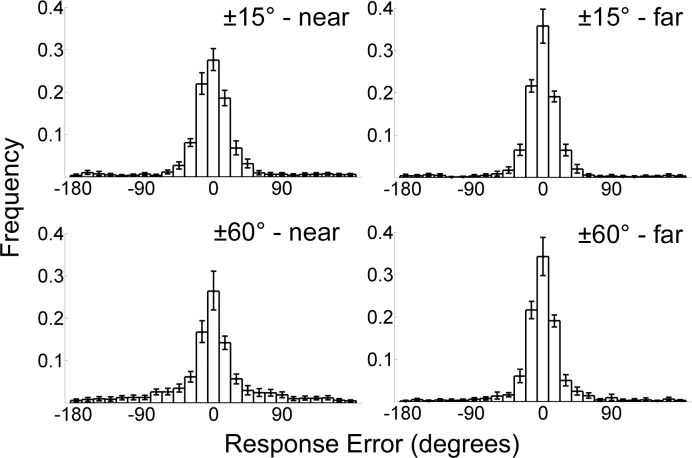
Schematics of the target displays used in this experiment are shown in Figure 5. Experiment 2 was similar to Experiment 1 with the following exceptions: First, when present, distractors were tilted ±15° or ±60° relative to the target. Second, in 50% of crowded trials, the center-to-center distance between the target and distractors was set at 3.33° (identical to Experiment 1; “near” trials); in the remaining 50% of trials, this distance was increased to 6.50° (“far” trials). Target eccentricity was fixed at 9.67°. Data were fit using the averaging and substitution models described in Equations 1 and 2.

Figure 5.

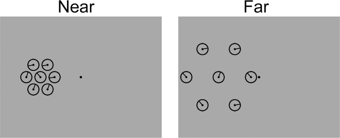
Target displays used in Experiment 2. Displays are not drawn to scale; see Methods for information on display parameters.

Results

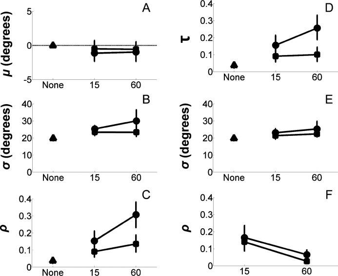
The mean distribution of response errors during uncrowded trials is shown in Figure 2B. As in Experiment 1, response errors were tightly distributed around 0 with few high-magnitude errors. Next, we fit each participant's distribution of response errors within each of the four crowded conditions with the averaging and substitution models described in Equations 1 and 2. Histograms of response errors within each crowded condition are shown in Figure 6, and the parameters for the best-fitting averaging and substitution models are shown in Figure 7. As in Experiment 1, BMC was used to compare the performance of the two models within each crowded condition. Unlike Experiment 1, both models performed equally well in all conditions. For example, the difference in model log likelihoods (substitution minus averaging) for the near and far ±15° and ±60° conditions were 0.36, 0.53, −0.67, and 0.16, respectively. We thus examined the plausibility of the averaging and substitution models as a function of target–distractor tilt (i.e., ±15° or ±60°) by comparing estimates of μ, σ, and ρ (for the averaging model) and σ, τ, and ρ (for the substitution model) during crowded and uncrowded trials (separately for near and far trials) using the same logic outlined in Experiment 1.

Figure 6.

Histograms of response errors observed in each condition of Experiment 2. Error bars are 95% confidence intervals.

Figure 7.

Pooling and substitution model parameters obtained in Experiment 2. (A, B, and C) Estimates of μ, σ, and ρ obtained from the pooling model in Equation 1 as a function of distractor presence (triangle symbols) and target–distractor differences (±15° and ±60°). (D, E, and F) Estimates of τ, σ, and ρ obtained from the substitution model in Equation 2 as a function of distractor presence (triangle symbols) and target–distractor differences. By definition, τ = 0 when there are no distractors in this display, so this condition has been omitted from (D). The estimate of σ for uncrowded trials in (E) was obtained via the pooling model, i.e., it is identical to the estimate shown in (B). Lines connected by squares correspond to “far” trials, and lines connected by circles correspond to the “near” trials. Error bars are 95% confidence intervals.

We began by examining the behavior of the simple averaging model. Target–distractor tilt had no effect on estimates of μ in either the near or far condition (p = 0.60 and 0.33, bf = 0.22 and 0.36, respectively). Conversely, tilt had a substantial effect on estimates of σ during both near and far trials (p = 3.30e − 05 and 8.45e − 04, bf = 560 and 61.29 for ±15° and ±60° trials, respectively). Post hoc analyses on σ revealed substantially lower estimates during both ±15° and ±60° near trials relative to uncrowded trials (p = 6.61e − 05 and 0.004; bf = 407.17 and 72.59, respectively), but the difference between ±15° and ±60° trials was not significant (p = 0.93, bf = 0.24). Similar findings were observed for far trials. Specifically, we observed reliably lower estimates of σ during ±15° and ±60° trials relative to uncrowded trials (p = 2.94e − 06 and 0.004, bf = 6,697 and 11.55 for ±15° and ±60° trials, respectively). The difference between ±15° and ±60° trials was not significant (p = 0.11; bf = 9.77). Finally, an ANOVA on estimates of ρ revealed significant effects of target–distractor tilt during both near and far trials (p = 3.18e − 06 and 3.50e − 11, bf = 4,881 and 6.71e + 08, respectively).

As in Experiment 1, the substantial increases in estimates of σ from uncrowded to both near and far crowded trials are inconsistent with a simple feature-averaging model in which items are averaged prior to reaching awareness. However, the current data can be accommodated by a substitution model with which targets and distractors are occasionally “swapped,” leading participants to report a distractor value as the target. Thus, we examined the behavior of this model in more detail. Specifically, separate 2 × 2 ANOVAs with target–flanker rotation (±15°, ±60°) and target–flanker distance (near, far) as within-participants factors were performed on estimates of σ, τ, and ρ. For σ, this analysis revealed a marginally significant main effect of distance (p = 0.05) but no main effect of rotation (p = 0.20) nor an interaction between these factors (p = 0.76). A complementary Bayesian ANOVA revealed very modest support for a model containing only the main effect of distance (bf = 1.88 relative to the null hypothesis of no main effects nor an interaction).

An identical analysis performed on estimates of τ revealed a main effect of target–flanker rotation, (p = 7.42e − 04) but no main effect of distance (p = 0.15) nor an interaction (p = 0.77). A Bayesian ANOVA revealed strong support for a model containing only target–distractor rotation relative to a null model containing no main effects nor an interaction (bf = 1,919) but relatively weak support when compared to the next strongest model containing both main effects (bf = 1.72). Finally, the same analysis on estimates of ρ revealed a main effect of rotation (p = 4.33e − 04), a main effect of distance (p = 8.17e − 05), and a significant interaction between these factors (p = 1.18e − 04). A complementary Bayesian ANOVA revealed strong support for a model containing both main effects and their interaction (bf = 1.61e + 07 relative to a null model containing no effects and bf = 8.19 relative to the next strongest model containing both main effects but not their interaction). Visual inspection of Figure 7F suggests that random responses were more likely during near relative to far trials.

To summarize, the results of Experiment 2 largely replicate those of Experiment 1: Although BMC revealed equivalent support for the averaging and substitution models, a comparison of parameter estimates returned by the averaging model across crowded and uncrowded trials revealed evidence inconsistent with averaging. Specifically, the precision of participants' response errors decreased with increasing target–distractor rotation. Because an equal number of distractors were tilted clockwise and counterclockwise relative to the target, one would expect performance to be as good when crowders are present relative to when they are not under an averaging model. This was not the case. Finally, Experiment 2 revealed that increasing target–distractor spatial separation—a factor known to have a large influence on crowding strength—reduced the frequency of random orientation reports but had little effect on the precision of participants' responses or the likelihood of reporting a distractor orientation.

Discussion

In two experiments, we examined whether crowding-induced changes in a continuous orientation report task were better explained by a model assuming feature averaging or a model assuming a probabilistic substitution of target and flanker features. In Experiment 1, the substitution model outperformed the averaging model when target–distractor similarity was low, replicating the results of an earlier study (Ester et al., 2014). However, when similarity was high, both models performed equally well. A comparison of parameter estimates returned by the averaging model across crowded and uncrowded trials revealed evidence inconsistent with simple feature averaging. Specifically, the relative precision of participants' orientation reports decreased during crowded relative to uncrowded trials. Moreover, precision decreased monotonically with the angular difference between target and flanker orientations. Both of these results are inconsistent with an averaging model in which each stimulus (flanker or target) contributes equally to the ultimate perception of orientation. Specifically, recall that when present, half of the crowders were tilted counterclockwise relative to the target, and the remaining crowders were tilted clockwise relative to the target by an equivalent amount. If each orientation contributes equally to the computation of a local average, then one would expect orientation report performance for crowded displays to equal or exceed performance for uncrowded displays. We also found no evidence for an averaging model in which “inner” or “outer” flankers are weighted more heavily during the averaging operation. Experiment 2 replicated these findings while manipulating a factor known to influence the severity of crowding: target–flanker distance. Increasing the separation between the target and nearby distractors had a large effect on the frequency of random responses in the model but little effect on either the likelihood of nontarget reports or the precision of participants' responses.

Here, we compared a simple pooling model in which the target and distractor orientations are averaged prior to reaching awareness (Parkes et al., 2001; see also Greenwood et al., 2009) with a substitution model in which the target and a neighboring flanker are occasionally swapped (Ester et al., 2014). Although either of these alternatives may often suffice to explain the pattern of errors observed in a given crowding experiment, other models are also plausible. One possibility is that participants encode and/or report targets and distractors with variable precision over trials (e.g., van den Berg et al., 2012). On the one hand, it is difficult to fathom how such a model could explain the clearly trimodal distribution from the ±90° condition in Experiment 1 (Figure 3D). On the other hand, such a model could easily mimic either pooling or substitution when target–distractor similarity is high. Additional research is needed to evaluate this possibility.

As mentioned in the Introduction, feature averaging constitutes just one example of “pooling.” Other forms of pooling include positional averaging (e.g., Dakin et al., 2010; Greenwood et al., 2009) and pixel averaging (e.g., Balas et al., 2009). Each of these alternatives have been invoked to explain crowding effects under various scenarios, but we suspect that many of these demonstrations can also be accounted for by probabilistic substitution. Consider a study by Greenwood et al. (2009) in which participants were asked to report the location of the horizontal stroke of a cross-like stimulus that was flanked by two cross-like distractors and reported that estimates of stroke position were systematically biased by the position of the distractors' strokes. This result is amenable to positional averaging, but it instead may reflect interactions of two response biases. Specifically, Greenwood et al. documented a repulsion bias from the target midpoint (i.e., participants rarely reported the target as a “+”), and we suspect that many participants may have had a similar bias away from extreme stroke positions (e.g., “T”) although this is impossible to ascertain from the data. Nevertheless, the combination of these biases could restrict the range of possible responses and create the artificial appearance of positional averaging.

More recent theoretical and experimental work suggests that pooling may reflect a nonlinear combination of local first- and second-order statistics, resulting in a “mongrel” percept that resembles any or none of the original stimuli (e.g., Balas et al., 2009; Freeman & Simoncelli, 2011). Our findings neither refute nor support this possibility. However, one potential limitation of these studies is that they rely on forced-choice identification or discrimination tasks that preclude participants from reporting precisely what they perceive in each trial (e.g., a participant cannot report that his or her mongrel percept “looks like the average of an H and a B”). Under many circumstances, it may be desirable or useful to examine the effects of flankers on perception by asking participants to directly report target features. For example, the analytical approach used in the current study allows one to account for a large range of possible responses by estimating the precision and relative frequencies of target and nontarget responses as well as the frequency of random orientation reports. Related approaches may be intractable for some stimulus sets (e.g., letters or natural images), but where possible, they may yield novel insights that complement or refute data patterns observed in forced-choice tasks.

The present findings build upon recent work challenging feature averaging as a major cause of visual crowding (Anderson, Ester, Klee, Vogel, & Awh, 2014; Ester et al., 2014). Specifically, we have shown that a probabilistic substitution model outperforms a pooling model when target–distractor similarity is low, replicating earlier findings (Anderson et al., 2014; Ester et al., 2014). However, a systematic comparison of pooling-model parameters during uncrowded and crowded trials revealed evidence inconsistent with a simple feature-averaging model. Instead, the data can be accommodated by a probabilistic substitution model, which assumes that crowding manifests when participants accidentally “swap” a target for a distractor.

References

- Abramowitz M., Stegun I. A. (Eds.) (1964). Handbook of mathematical functions. Washington, D.C.: National Bureau of Standards. [Google Scholar]
- Anderson D. E., Ester E. F., Klee D., Vogel E. K., Awh E. (2014). Electrophysiological evidence for failures of item individuation in crowded visual displays. Journal of Cognitive Neuroscience , 26, 2298–2309. [DOI] [PMC free article] [PubMed] [Google Scholar] [Retracted]
- Balas B., Nakano L., Rosenholtz R. (2009). A summary statistic representation in peripheral vision explains visual crowding. Journal of Vision , 9 (12): 4 1–18, http://www.journalofvision.org/content/9/12/13, doi:10.1167/9.12.13. [DOI] [PMC free article] [PubMed] [Google Scholar]
- Bouma H. (1970). Interaction effects in parafoveal letter recognition. Nature , 226, 177–178. [DOI] [PubMed] [Google Scholar]
- Brainard D. H. (1997). The psychophysics toolbox. Spatial Vision , 16, 433–436. [PubMed] [Google Scholar]
- Carrasco M., Evert D. L., Chang I., Katz S. M. (1995). The eccentricity effect: Target eccentricity affects performance on conjunction search. Attention, Perception & Psychophysics , 57, 1241–1261. [DOI] [PubMed] [Google Scholar]
- Chastain G. (1982). Confusability and interference between members of parafoveal letter pairs. Attention, Perception & Psychophysics , 32, 576–580. [DOI] [PubMed] [Google Scholar]
- Chung S. T. L. (2002). The effect of letter spacing on reading speed in central and peripheral vision. Investigative Ophthalmology & Visual Science , 43, 1270–1276, http://www.iovs.org/content/43/4/1270. [PubMed] [Google Scholar]
- Dakin S. C., Cass J., Greenwood J. A., Bex P. J. (2010). Probabilistic positional averaging predicts object-level crowding effects with letter-like stimuli. Journal of Vision , 10 (10): 4 http://www.journalofvision.org/content/10/10/14, doi:10.1167/10.10.14. [DOI] [PMC free article] [PubMed] [Google Scholar]
- Edwards W., Lindman H., Savage L. J. (1963). Bayesian statistical inference for psychological research. Psychological Review , 70, 193–242. [Google Scholar]
- Ehlers H. (1936). The movements of the eyes during reading. Acta Opthalmologica , 14 (4), 56–63. [Google Scholar]
- Ester E. F., Klee D., Awh E. (2014). Visual crowding cannot be wholly explained by feature pooling. Journal of Experimental Psychology: Human Perception & Performance , 40, 1022–1033. [DOI] [PMC free article] [PubMed] [Google Scholar]
- Fisher N. I. (1993). Statistical analysis of circular data. New York: Cambridge. [Google Scholar]
- Freeman J., Simoncelli E. (2011). Metamers of the ventral stream. Nature Neuroscience , 14, 1195–1201. [DOI] [PMC free article] [PubMed] [Google Scholar]
- Greenwood J. A., Bex P. J., Dakin S. C. (2009). Positional averaging explains crowding with letter-like stimuli. Proceedings of the National Academy of Sciences, USA , 106, 13130–13135. [DOI] [PMC free article] [PubMed] [Google Scholar]
- Kass R. E., Raftery A. E. (1995). Bayes factors. Journal of the American Statistical Association , 90, 773–795. [Google Scholar]
- Levi D. (2008). Crowding – An essential bottleneck for object recognition: A mini-review. Vision Research , 48, 635–654. [DOI] [PMC free article] [PubMed] [Google Scholar]
- MacKay D. J. (2003). Information theory, inference, and learning algorithms. Cambridge, UK: Cambridge University Press. [Google Scholar]
- Mareschal I., Morgan M. J., Solomon J. A. (2010). Cortical distance determines whether flankers cause crowding or the tilt illusion. Journal of Vision , 10 (8): 4 1–14, http://www.journalofvision.org/content/10/8/13, doi:10.1167/10.8.13. [PubMed] [Article] [DOI] [PubMed] [Google Scholar]
- Parkes L., Lund J., Angelucci A., Solomon J. A., Morgan M. (2001). Compulsory averaging of crowded orientation signals in human vision. Nature Neuroscience , 4, 739–744. [DOI] [PubMed] [Google Scholar]
- Pelli D. G. (1997). The VideoToolbox software for visual psychophysics: Transforming numbers into movies. Spatial Vision , 10, 437–442. [PubMed] [Google Scholar]
- Pelli D. G. (2008). Crowding: A cortical constraint on object recognition. Current Opinion in Neurobiology , 18, 445–451. [DOI] [PMC free article] [PubMed] [Google Scholar]
- Pelli D. G., Tillman K. A., Freeman J., Su M., Berger T. D., Majaj N. J. (2007). Crowding and eccentricity determine reading rate. Journal of Vision , 7 (2): 4 1–36, http://www.journalofvision.org/content/7/2/20, doi:10.1167/7.2.20. [PubMed] [Article] [DOI] [PubMed] [Google Scholar]
- Scolari M., Kohnen A., Barton B., Awh E. (2007). Spatial attention, preview, and popout: Which factors influence critical spacing in crowded displays? Journal of Vision , 7 (2): 4 1–23, http://www.journalofvision.org/content/7/2/7, doi:10.1167/7.2.7. [PubMed] [Article] [DOI] [PubMed] [Google Scholar]
- Strasburger H., Harvey L. O., Rentschler I. (1991). Contrast thresholds for identification of numeric characters in direct and eccentric view. Perception & Psychophysics , 49, 495–508. [DOI] [PubMed] [Google Scholar]
- Strasburger H., Malania M. (2013). Source confusion is a major cause of crowding. Journal of Vision , 13 (1): 4 1–20, http://www.journalofvision.org/content/13/1/24, doi:10.1167/13.1.24. [PubMed] [Article] [DOI] [PubMed] [Google Scholar]
- Strasburger H., Rentschler I., Jüttner M. (2011). Peripheral vision and pattern recognition: A review. Journal of Vision , 11 (5): 4 1–82, http://www.journalofvision.org/content/11/5/13, doi:10.1167/11.5.13. [PubMed] [Article] [DOI] [PMC free article] [PubMed] [Google Scholar]
- Stuart J., Burian H. (1962). A study of separation difficulty: Its relationship to visual acuity in the normal amblyopic eye. American Journal of Ophthalmology , 53, 163–169. [PubMed] [Google Scholar]
- van den Berg R., Roerdink J. B. T. M., Cornelissen F. (2010). A neurophysiologically plausible population code model for feature integration explains visual crowding. PLoS Computational Biology , 6, 1–10. [DOI] [PMC free article] [PubMed] [Google Scholar]
- van den Berg R., Shin H., Chou W.-C., George R., Ma W. J. (2012). Variability in encoding precision accounts for visual short-term memory limitations. Proceedings of the National Academy of Sciences, USA , 109, 8780–8785. [DOI] [PMC free article] [PubMed] [Google Scholar]
- Vlaskamp B. N. S., Hooge I. T. C. (2006). Crowding degrades saccadic search performance. Vision Research , 46, 417–425. [DOI] [PubMed] [Google Scholar]
- Wasserman L. (2000). Bayesian model selection and model averaging. Journal of Mathematical Psychology , 44, 92–107. [DOI] [PubMed] [Google Scholar]