FiberDock: Flexible induced-fit backbone refinement in molecular docking

Abstract

Upon binding, proteins undergo conformational changes. These changes often prevent rigid-body docking methods from predicting the 3D structure of a complex from the unbound conformations of its proteins. Handling protein backbone flexibility is a major challenge for docking methodologies, as backbone flexibility adds a huge number of degrees of freedom to the search space, and therefore considerably increases the running time of docking algorithms. Normal mode analysis permits description of protein flexibility as a linear combination of discrete movements (modes). Low-frequency modes usually describe the large-scale conformational changes of the protein. Therefore, many docking methods model backbone flexibility by using only few modes, which have the lowest frequencies. However, studies show that due to molecular interactions, many proteins also undergo local and small-scale conformational changes, which are described by high-frequency normal modes. Here we present a new method, FiberDock, for docking refinement which models backbone flexibility by an unlimited number of normal modes. The method iteratively minimizes the structure of the flexible protein along the most relevant modes. The relevance of a mode is calculated according to the correlation between the chemical forces, applied on each atom, and the translation vector of each atom, according to the normal mode. The results show that the method successfully models backbone movements that occur during molecular interactions and considerably improves the accuracy and the ranking of rigid-docking models of protein–protein complexes. A web server for the FiberDock method is available at: http://bioinfo3d.cs.tau.ac.il/FiberDock.

INTRODUCTION

Proteins are flexible entities. This flexibility is reflected in the conformational variation shown in different crystallized 3D structures of the same protein. Many proteins were crystallized when interacting with another protein in a bound conformation, and by themselves in an unbound conformation. By comparing the 3D structures of a protein in its bound and unbound conformations, one can see conformational changes in both the side chains and the backbone.

In docking, our goal is to predict the structure of a complex of two (or more) biological molecules, often called receptor and ligand, given their unbound conformations. However, predicting only the rigid transformation, which places the unbound ligand on the interaction interface of the unbound receptor in the native orientation, is not sufficient. The resulting model of the complex will often contain major steric clashes. Consequently, the calculated energy value of this near-native model will be very high and it will not be identified among a group of docking solution candidates. Additionally, the accuracy of such a model will often be poor, as without modeling the conformational changes of the proteins, the native chemical interactions, which are important for the complex formation, will not be attained in the model. Therefore, docking methods must model the conformational changes that proteins undergo upon binding, including both backbone and side-chain movements.

There are two main biological models that explain the structural differences between bound and unbound conformations of proteins. The first is called the conformational selection model.^1–5 According to this model, proteins constantly change conformations, and when, by chance, a protein, in its bound conformational state, encounters a complementary molecule, they interact and create a complex. The second model is called the induced-fit model.^6,7 This model postulates that the structures of the receptor and the ligand are partially compatible, and when they come into proximity of each other, the chemical forces created during their interaction induce their conformational changes. In nature, both models are likely to hold.⁸ The binding process begins with conformational selection, followed by an induced fit, which likely plays a role in local side chain and relatively minor backbone changes to optimize the associatio.⁹ Docking algorithms should mimic molecular recognition.¹⁰ The conformational selection model can be mimicked by performing cross rigid-docking using pregenerated ensembles of conformations of the receptor and the ligand^8,11–14 or by the mean-field approach.^15,16 The induced-fit model can be mimicked by performing flexible refinement of the rigid-docking candidate solutions by molecular dynamics,^17–20 energy minimization,^20,21 Monte-Carlo (MC) technique^14,22,23 normal mode-based methods,^24,25 etc.

Normal mode analysis (NMA)^26–28 is a commonly used method for analyzing the flexibility of a protein, given a single 3D structure, such as that of the unbound conformation. The analysis, described in detail in the Methods section, provides a set of possible movements, called normal modes, of the protein backbone and their vibration frequencies. The lowest frequency normal modes usually describe the large conformational changes a protein can undergo.^29–32

Lindahl and Delarue²⁴ refined near-native complex models by minimizing along the 5–10 lowest frequency normal mode directions. The method was tested on protein–small molecule and protein–DNA complexes with the unbound conformation of the receptors and bound conformation of the ligands. The refinement protocol was shown to significantly improve the root mean square deviation (RMSD) between the receptor’s modeled structure and its bound conformation. May and Zacharias²⁵ performed systematic protein–protein docking, starting with thousands of orientations of the ligand around the receptor and refining each one by minimizing the interaction energy along five of the lowest frequency normal modes. The method was shown to improve both the RMSD and the ranking of the solution closest to the native structure when compared with rigid docking.

Petrone and Pande³¹ attempted to assess the number of the lowest frequency normal modes that should be used to model the conformational changes between the unbound and bound conformations of proteins. They showed that the first 20 modes can only improve the RMSD to the bound conformation by up to 50% (in four test cases). The suggested reason was that while an unbound protein is likely to move in the directions of low-frequency normal modes, an interaction with another molecule often activates movements in the directions of high-frequency normal modes. Thus, high-frequency normal modes should be taken into account in flexible docking refinement methods.

Cavasotto et al.³³ used high-frequency normal modes to model loop flexibility in binding pockets of cAPK kinases. They developed a measure of relevance of a normal mode to a loop of interest. Using this measure, they identified a small set of relevant normal modes that were used to generate an ensemble of possible loop conformations. When compared with rigid docking, an ensemble cross-docking improved the docking accuracy. In addition, binders identification was improved in a small-scale virtual screening.

In this article, a new method, called FiberDock, for flexible refinement is presented. The method allows both backbone and side-chain flexibility. It minimizes the structural conformations of the interacting proteins and optimizes their rigid-body orientation. The side-chain flexibility is modeled by a rotamer library, and the backbone flexibility is modeled by an a priori unlimited number of normal modes. The method iteratively minimizes the structure of the flexible protein along the most relevant modes. The relevance of a mode is calculated according to its correlation with the chemical forces applied on each atom. The results, detailed later, show that the method considerably improves the accuracy and the ranking of rigid-docking models of protein–protein complexes. In addition, we compared FiberDock to our previously developed refinement method FireDock³⁴ and to the RosettaDock method.³⁵ Both model only side-chain movements and keep the backbone rigid. This comparison showed that the modeling of backbone flexibility in the refinement process is often critical for creating near-native models with low energy values.

METHODS

Docking refinement aims to refine docking solution candidates and rerank them to identify near-native models. The refinement has to take into account both backbone and side-chain flexibility. The new method, FiberDock (flexible induced-fit backbone refinement in molecular docking), presented here combines a novel NMA-based backbone flexibility treatment with our previously developed flexible side-chain refinement technique, FireDock.³⁴ Currently, the refinement algorithm models backbone flexibility in one of the proteins (the receptor) and side-chain flexibility in both of them. The algorithm, described in the flowchart in Figure 1, contains the following steps:

Figure 1.

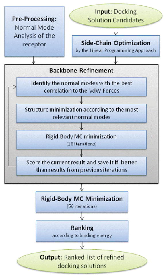
1. Preprocessing: Normal mode analysis of the flexible protein (the receptor) using the anisotropic network model (ANM).²⁷

2. For each docking solution candidate do:

   1. Side-chain optimization: Side-chain flexibility of interface residues of both proteins is modeled by a rotamer library. The optimal combination of rotamers is found by an integer linear programming (ILP) technique.³⁶ At the end of this stage, a rigid body minimization is performed by the BFGS quasi-Newton algorithm.^37,38

   2. NMA-based backbone refinement: The backbone refinement performs up to N iterations which consist of the following steps: (1) The van der Waals (vdW) forces that the ligand applies on the receptor are calculated. (2) The 10 normal modes with the best correlation to these forces are identified, and the receptor’s backbone conformation is minimized along these modes. (3) Ten Monte-Carlo (MC) iterations of rigid-body minimization are performed (as described in item 2c). (4) A score is calculated for the current result and the result is saved if it is superior to the results from previous iterations. The iterative process of the backbone refinement step stops if the repulsive van der Waals (repVdW) energy value of the current result is below a threshold (no significant steric clashes) or if there was no improvement in the result in the last five iterations.

   3. Rigid body MC minimization: The rigid-body orientation of the ligand is optimized by a MC technique (50 iterations), and a BFGS quasi-Newton minimization is performed in each MC cycle.^37,38

3. Ranking according to an approximation of the energy function: This stage attempts to identify near-native solutions among the entire set of refined complexes.

In the evaluation experiments, detailed in the Results section, up to 20 iterations of backbone refinement were performed (N = 20), and the normal modes with the best correlation to the repVdW forces were chosen out of the first 200 modes, with the lowest frequencies. The running time of the refinement algorithm on a single docking solution varies between 1 and 50 s (average of 14 s) depending on the size of the receptor.

The implementation of the side-chain optimization (item 2a) and the rigid-body MC minimizations (item 2c) steps were adopted from the FireDock method.³⁴ The number of iterations performed in the rigid-body MC minimization step was chosen according to convergence rate of the minimization. The rest of the steps are detailed later.

Normal mode analysis

NMA enables us to describe protein flexibility as a linear combination of discrete movements.^26–28 Given a single conformation of a protein, the analysis provides a set of vectors (normal modes) that describe typical motions of the analyzed protein. Each normal mode vector contains 3N entries, where N is the number of atoms or Cα atoms in the protein, depending on the resolution of the analysis. The entire set of normal modes spans the conformational space of the protein, that is, any conformation can be expressed as a linear combination of normal modes. The coefficient of a normal mode represents its amplitude. In addition, the analysis provides the vibration frequency of each mode. The low-frequency modes usually describe the large scale motions of the protein.

In general, normal modes are calculated as follows. First, the Hessian matrix (K) of the second derivative of the potential energy (U) of each atom in each axis is calculated as follows:

$$K_{ij}=\frac{{\partial }^{2}U}{\partial r_i\partial r_j}.$$ (1)

The size of the matrix is 3N × 3N, where N is the number of atoms. r_i denotes the position of atom i in the minimal energy conformation. Then, the matrix is converted to mass-weighted coordinates according to the formula:

$$\stackrel{\sim }{K}={\sqrt{M}}^{-1}·K·{\sqrt{M}}^{-1},$$ (2)

where M is a diagonal 3N × 3N matrix containing the atomic masses. The normal modes are the eigenvectors of this matrix (K̃). The vibration frequencies are the square roots of the corresponding eigenvalues.

The Anisotropic Network Model (ANM) is a simplified spring model of a protein, which is commonly used for NMA.^27,39 This model is based on a pairwise harmonic potential function, which is calculated for atom pairs whose distance from each other is below a threshold. The model treats the analyzed structure as the equilibrium conformation, as opposed to the original all-atom-based NMA which requires prior energy minimization. The harmonic potential function is detailed in Eq. 3, where R_i is the position of atom i, and $R_i^0$ is the position of atom i in the equilibrium conformation. k_ij denotes the force coefficient of the spring, which connects atoms i and j in the model.

$$\begin{array}{l}U(R_1,\dots ,R_N)={\sum }_{i,j}{U}_{ij}(R_i-Rj),\\ U_{ij}(r)=k_{ij}{(\mid r\mid -\mid (R_i^0-R_j^0)\mid )}^2.\end{array}$$ (3)

In this work, we used the NMA software developed by Lindahl et al.²⁴ The software uses the ANM with force coefficients that decay exponentially with distance, as detailed in Eq. 4. The analysis was performed on the Cα atoms with screening length (r₀) of 3 Å and a distance cutoff of 10 Å.

$$k_{ij}=exp\left(-\frac{\mid R_i^0-R_j^0{\mid }^2}{r_0^2}\right).$$ (4)

Correlation measurement

In each iteration of the backbone refinement procedure, the normal modes with the best correlation to the repVdW forces are applied on the flexible protein. The application of the repVdW forces only produced better results (i.e., more accurate backbone movements and more accurate docking results) when compared with the application of the full van der Waals forces. This is probably due to the fact that the correlation to the repVdW forces helps us choose normal modes that describe backbone movements that resolve existing steric clashes, which often prevent docking methods from succeeding. Resolving steric clashes in near-native rigid-docking solutions drastically improves the energy score of the model, enabling it to be highly ranked and therefore identified among a group of hundreds or thousands solution candidates. Normal modes that correlate well with attractive vdW forces often describe unrealistic closing motions of the receptor around the ligand. We believe that attractive vdW forces can still improve the results when used with certain regularization factors (yet to be found) and plan to continue investigating the optimal application of these forces along with other attractive forces in the future.

The vdW forces are calculated according to the derivative of the modified Lennard-Jones 6–12 potential with linear short-range repulsive score.³⁵ Specifically, the value of the vdW force between atom a_i and a_j is calculated as follows:

$$\begin{array}{l}{F}_{\text{vdW}}(a_i,a_j)=\{\begin{array}{ll}-12{\epsilon }_{ij}\frac{{\sigma }_{ij}^6}{r_{ij}^7}\left(\frac{{\sigma }_{ij}^6}{r_{ij}^6}-1\right)\hfill & \text{for}{r}_{ij}>0.6{\sigma }_{ij}\hfill \\ -{\epsilon }_{ij}B\hfill & \text{otherwise},\hfill \end{array}\\ \text{where}B=\frac{12}{{0.6}^7}\left(\frac{1}{{\sigma }_{ij}}-\frac{1}{{0.6}^6}\right).\end{array}$$ (5)

The parameter σ_ij is the sum of the radii of the two atoms. The parameter ε_ij is the energy well depth, and its value was taken from CHARMM22 force field parameters.⁴⁰

A vdW force that a ligand atom applies on a receptor atom is considered to be repulsive if it pushes the receptor atom in a direction opposite to the ligand atom. The repVdW forces that are applied on the atoms of a certain amino acid are summed, and the resulting force vector is assigned to the Cα atom of that amino acid.

The correlation between the forces (F) that are applied on the Cα atoms and a certain normal mode (V_i) is calculated as follows:

$$\text{corr}(\mathit{F},{\mathit{V}}_{\mathit{i}})=\left|\frac{1}{\widehat{m}·{(V_i^{\text{freq}})}^2}\sum _{j=0}^m\overrightarrow{v_{ij}}·\overrightarrow{f_j}\right|,$$ (6)

where m is the number of Cα atoms in the receptor, and m̂ is the number of Cα atoms on which a vdW force is applied ( $\widehat{m}=\mid \{\overrightarrow{f_j}:\mid \overrightarrow{f_j}\mid >\epsilon ,j=\mathrm{1..}m\}\mid$). $\mathit{F}=(\overrightarrow{f_1},\dots ,\overrightarrow{f_m})$ are the repVdW forces applied on the Cα atoms, and ${\mathit{V}}_{\mathit{i}}=(\overrightarrow{v_{i1}},\dots ,\overrightarrow{v_{im}})$ are the displacement vectors of each Cα atom according to the i^th normal mode. $V_i^{\text{freq}}$ denotes the frequency value of the i^th normal mode.

The absolute value of the dot product $\overrightarrow{v_{ij}}·\overrightarrow{f_j}$ is higher when the angle between the force vector and the normal mode vector (or its inverse vector) is smaller. Therefore, high correlation indicates that the forces and the normal mode vectors are in similar directions. Additionally, the absolute value of the dot product is higher when the force is stronger (the vector’s l₂ norm is bigger). Hence, the correlation measurement gives higher weight to an agreement with the direction of strong vdW forces. Moreover, the division by ${(V_i^{\text{freq}})}^2$ increases the correlation value of the lowest frequency normal modes and therefore gives them a higher priority.

Minimization according to normal modes

In each iteration of the backbone refinement procedure, the 10 most relevant normal modes, chosen by the correlation measurement described earlier, and the six rigid-body degrees of freedom, represented as six modes that describe translation and rotation movement along the three axes, are used for minimizing the structure of the complex (overall, 16 degrees of freedom). The energy function of the structure minimization procedure is composed of the attractive and repulsive van der Waals energy and a penalty deformation energy term that prevents the minimization from over-distorting the structure. The function is specified in Eq. 7.

$$E=K{E}_{\text{attrVdW}}+E_{\text{repVdW}}+\mathrm{\lambda }\sum _{i=1}^M{(V_i^{\text{freq}})}^2\mid V_i^{\text{amp}}\mid ,$$ (7)

where K is the weight of the attractive van der Waals term in the energy function. The choice of K = 5 yields the best performance results. M denotes the number of normal modes, the parameter λ is a scaling factor which was set to 0.05. $V_i^{\text{freq}}$ denotes the frequency of the i^th normal mode (the frequency of the rigid-body modes is zero), and $V_i^{\text{amp}}$ denotes its amplitude. The vdW energy values are calculated according to the modified Lennard-Jones 6–12 potential with linear short-range repulsive score.³⁵ If the vdW energy between two atoms is a positive number, then it is added to the repulsive van der Waals term E_repVdW, otherwise to the attractive van der Waals term E_attrVdW.

Using BFGS quasi-Newton algorithm^37,38 we find the optimal amplitudes of the 10 minimized normal modes and the six rigid body degrees of freedom, which result in the nearest local energy minimum. The algorithm uses the gradient of the energy function above. The gradient in the direction of normal mode V_i is specified in Eq. 8

$$\frac{dE}{d{\overrightarrow{V}}_i^{\text{amp}}}=\{\begin{array}{cc}{\sum }_{j=0}^m\overrightarrow{v_{ij}}·\overrightarrow{f_j}+\mathrm{\lambda }{(V_i^{\text{freq}})}^2,& \text{if}{V}_i^{\text{amp}}>0.\\ {\sum }_{j=0}^m\overrightarrow{v_{ij}}·\overrightarrow{f_j}-\mathrm{\lambda }{(V_i^{\text{freq}})}^2,& \text{if}{V}_i^{\text{amp}}<0,\end{array}$$ (8)

where ${\overrightarrow{V}}_i^{\text{amp}}$ is the normal mode V_i multiplied by its amplitude, m is the number of Cα atoms in the receptor, $\overrightarrow{f_1},\dots ,\overrightarrow{f_m}$ are the vdW forces applied on the Cα atoms (the attractive forces are multiplied by K), and $\overrightarrow{v_{i1}},\dots ,\overrightarrow{v_{im}}$ are the displacement vectors of each Cα according to the i^th normal mode. At the end of each structure minimization step, we apply the normal modes on the flexible protein with the optimal amplitudes found, as described later.

Applying a normal mode on a protein

A normal mode ${\mathit{V}}_{\mathit{i}}=(\overrightarrow{v_{i1}},\dots ,\overrightarrow{v_{im}})$ is composed of displacement vectors for each Cα atom in a protein. When applying normal mode movements on a protein in a naïve manner, that is, by adding the displacement vectors, multiplied by an amplitude value, to the points of the Cα atom, the protein structure often distorts. We would like to change the conformation of the protein according to certain normal modes while preserving the bond lengths and angles, that is, by allowing a change only in the backbone dihedral angles, ϕ and ψ.

To overcome this problem, we use a modification of the CCD algorithm,⁴¹ a robotics algorithm which was adapted for protein loop closure. First, we add the displacement vectors of the normal modes to the centers of the Cα atoms and get the desired positions of the atoms, denoted by (a₁,…,a_m). Then we start from the Cα atom that moves the least (Cα_j, where j = argmin|v_ij|) and change the values of the backbone dihedral angles ϕ and ψ in a sequential order in both directions of the backbone chain. For each dihedral angle (θ) of Cα_k, we choose the value that minimizes the sum of the squared distances between the next three moving Cα atoms (c_k±1, c_k±2, c_k±3) and their desired positions (a_k±1, a_k±2, a_k±3) [Eq. 9]. The value of each angle is calculated by setting the first-order derivative of the sum of the square distances to zero (dS/dθ = 0), as described by Canutescu and Dunbrack.⁴¹

$$S(\mathrm{\theta })={[\mathrm{d}(c_{k\pm 1},a_{k\pm 1})]}^2+{[\mathrm{d}(c_{k\pm 2},a_{k\pm 2})]}^2+{[\mathrm{d}(c_{k\pm 3},a_{k\pm 3})]}^2.$$ (9)

The scoring function of the backbone refinement stage

At the end of each iteration in the backbone refinement procedure, a score is calculated for the current solution, and the solution with the best score is returned from the procedure. This scoring function is identical to the energy function specified in Eq. 7.

Ranking according to an approximation of the energy function

This stage attempts to identify near-native solutions among the entire set of refined complexes. The calculated energy score is an approximation of the binding free energy function. It includes an interface energy score, adopted from the FireDock method,³⁴ and an energy term that approximates the internal deformation energy of the flexible protein (the receptor). The interface energy score includes a variety of energy terms, such as desolvation energy (ACE), van der Waals interactions, partial electrostatics, hydrogen and disulfide bonds, π-stacking, aliphatic interactions, and more. These terms are described in detail in the FireDock paper.³⁴ The added deformation energy term approximates the energy required for deforming the unbound backbone structure of the flexible protein according to the calculated linear combination of the chosen relevant normal modes. This term is specified in Eq. 10.

$$E_{\text{deform}}=\sum _{i=1}^M{(V_i^{\text{freq}})}^2\mid V_i^{\text{amp}}\mid ,$$ (10)

where $V_i^{\text{freq}}$ denotes the frequency of the i^th normal mode and $V_i^{\text{amp}}$ denotes its amplitude. The deformation energy term, E_deform, is added to the interface energy function with a weight of λ = 0.05.

RMSD calculations

The root mean square deviation (RMSD) is a common measure of the difference between structures of two proteins (or complexes). The RMSD is calculated according to the following equation:

$$\text{RMSD}=\sqrt{\frac{1}{n}\sum _{i=1}^n{\Vert v_i-u_i\Vert }^2}$$ (11)

where n is the number of atoms in the compared molecules, v_i is the position of the i^th atom of the first molecule, and u_i is the position of the corresponding atom in the second molecule. In this work, we evaluated the results by three types of RMSD measurements:

• LRMSD: The RMSD between the predicted location of the ligand and its location in the native complex. The calculation was performed on Cα atoms of the ligand after superimposing the receptor molecules in the native complex and in the predicted complex.

• IRMSD: The RMSD between the interface Cα atoms in the predicted complex structure and in the native complex structure after superimposing the two interfaces. The interface includes all the residues that contain an atom within 10 Å of the other interacting protein in the structure of the native complex, as defined in the evaluation protocol of the CAPRI experiment.⁴²

• Rec-IRMSD: The RMSD between the interface Cα atoms in a certain structure of the receptor and in the structure of its bound conformation (as in the native complex), after superimposing the two interfaces.

Test cases

We used 20 test systems in which the conformation of the receptor’s backbone changes upon interaction with the ligand. The test cases are detailed in Table I. The interface RMSD between the bound and the unbound conformations of the receptor (Rec-IRMSD) in this data set varies in the range of 0.59–6.08 Å. We classified the motions of the receptors into three types: (1) opening motion, where the conformation of the unbound receptor partially blocks the binding site of the ligand (nine cases); (2) closing motion, where the receptor closes around the ligand and increases the contact area (three cases); and (3) other motions, where some of the interface suits the opening criterion and some suits the closing criterion (eight cases). In most of the cases, an unbound structure of the ligand was available. In these cases, unbound–unbound docking experiments were performed.

Table I.

Flexible Protein–Protein Docking Data Set

No.	Complex ID	Unbound receptor	Unbound ligand	Complex description	Rec-IRMSD	Motion type
1	1A0O	1CHN	1FWP	CheY-binding domain of CheA in complex with CheY	2.12	Closing
2	1ACB	2CGA	1EGL	Bovine alpha-chymotrypsin-Eglin C complex	2.58	Other
3	1AY7	1RGH	1A19	Ribonuclease Sa complex with Barstar	0.59	Opening
4	1BTH	2HNT	6PTI	Thrombin complexed with bovine pancreatic trypsin inhibitor	1.31	Other
5	1CGI	2CGA	1HPT	Bovine chymotrypsinogen A and pancreatic secretory trypsin inhibitor	2.26	Other
6	1DFJ	2BNH	7RSA	Ribonuclease inhibitor complexed with ribonuclease A	1.18	Opening
7	1E6E	1E1N	1CJE	Adrenodoxin reductase-adrenodoxin complex	0.62	Other
8	1FIN	1HCL	1VIN	CyclinA-CDK2 complex	6.08	Opening
9	1GGI	1GGC	—	HIV-1 neutralizing antibody in complex with its V3 loop peptide antigen	1.67	Opening
10	1GOT	1TAG	1TBG	Heterotrimeric G protein	3.72	Opening
11	1IBR	1F59	1F59	Complex of Ran with Importin beta	2.62	Opening
12	1OAZ	1OAQ	—	Immunoglobulin E complexed with a Thioredoxin 1	1.07	Other
13	1PXV	1X9Y	1NYC	Staphostatin–Staphopain complex	3.48	Other
14	1T6G	1UKR	1T6E	Complex of endo-1,4-beta-xylanase I and xylanase inhibitor	0.87	Opening
15	1TGS	2PTN	1HPT	Complex of trypsinogen and pancreatic secretory trypsin inhibitor	1.54	Closing
16	1WQ1	6Q21	6Q21	Ras-RasGAP complex	0.93	Other
17	1ZHI	1M4Z	1Z1A	Complex of Orc1 and Sir1 interacting domains	0.74	Closing
18	2BUO	1A43	—	HIV-1 capsid C-terminal domain with an inhibitor of particle assembly	4.15	Opening
19	2KAI	2PKA	6PTI	Complex of porcine kallikrein A and the bovine pancreatic trypsin inhibitor	0.72	Other
20	3HHR	1HGU	—	Complex of a human growth hormone and extracellular domain of its receptor	2.62	Opening

RESULTS

To evaluate the contribution of the backbone flexibility modeling within the docking refinement process, we compared the performance of the new FiberDock method to the performance of our previously developed flexible side chain refinement technique, FireDock.³⁴ The only difference between the two methods is the addition of the novel NMA-based backbone refinement procedure in FiberDock (step 2b in the algorithm, described in “Methods” section). We performed three main experiments. In the first experiment, we tested the performance of the method on refining a complex structure, in which the ligand, in its unbound conformation, is placed in its native binding orientation and the receptor is in its unbound conformation. In the second experiment, we refined, for each test case, 500 randomly generated near-native docking solutions. Here, we compared FiberDock with both FireDock and RosettaDock,³⁵ and we investigated the influence of the backbone refinement procedure on the shape of the energy funnels created around the native binding orientation of the ligand. Finally, in the last experiment, we refined the best 500 results of the PatchDock rigid-body docking method,^43,44 and rescored the results. Ranking was identified as a major bottleneck in the CAPRI challange.^45–47 Therefore, in this last experiment, we aim to test to what extent FiberDock improves the ranking of the docking procedure.

Docking refinement starting from known binding orientation and unbound conformation of the proteins

In this experiment, we check the performance of the refinement method on the native complex structures after replacing the bound conformation of each protein with the superimposed unbound conformation. These complexes contain steric clashes due to the wrong conformation of the proteins. Therefore, their initial energy score is high. The refinement of the complex attempts to find a structurally close complex structure with minimal energy score. The results of the refinement are detailed in Table II.

Table II.

Refinement of the Unbound Receptor and Unbound Ligand in Their Native Binding Orientation

Complex ID	FireDock (rigid backbone)			FiberDock (flexible backbone)
	IRMSD	recIRMSD	Energy	IRMSD	recIRMSD	Energy
1. 1A0O	2.44	2.12	−14.81	2.44	2.12	−14.81
2. 1ACB	2.58	2.58	−46.23	2.57	2.54	−38.66
3. 1AY7	1.30	0.59	−40.53	1.30	0.59	−40.53
4. 1BTH	1.16	1.31	−42.15	1.16	1.31	−42.15
5. 1CGI	2.08	2.26	−52.61	2.08	2.26	−52.61
6. 1DFJ	1.41	1.18	−36.54	1.12	1.11	−30.02
7. 1E6E	1.21	0.62	−55.24	1.21	0.62	−55.24
8. 1FIN	5.17	6.08	813.84	6.06	6.16	0.3
9. 1GGI*	2.68	1.67	111.89	1.95	1.26	−51.79
10. 1GOT	3.02	3.72	107.25	4.68	3.78	−5.54
11. 1IBR	2.78	2.62	335.93	2.63	2.56	−17.32
12. 1OAZ*	1.00	1.07	4.35	1.00	1.07	4.35
13. 1PXV	3.54	3.48	11.55	3.42	3.31	−34.18
14. 1T6G	0.99	0.87	−10.39	0.88	0.66	−41.16
15. 1TGS	1.57	1.54	−43.28	1.57	1.54	−43.28
16. 1WQ1	1.50	0.93	2.50	1.50	0.93	2.50
17. 1ZHI	1.24	0.74	4.40	1.24	0.74	4.40
18. 2BUO*	3.92	4.15	−11.05	4.05	4.30	−32.71
19. 2KAI	0.74	0.72	−60.77	0.74	0.72	−60.77
20. 3HHR*	2.46	2.62	622.07	1.98	2.56	−9.9

^*For these cases, a structure of the ligand in its unbound conformation was not available. Therefore, the bound conformation of the ligand was used.

The results show that in many cases, FiberDock produced a near-native model with a much lower energy value when compared with FireDock. In five of the cases, the energy difference was very significant. These include case numbers 8, 9, 10, 11, and 20. In all of these cases, the receptor opens its binding site upon interaction with the ligand. Modeling these opening movements by Fiber-Dock resolved the steric clashes between the proteins in their unbound conformations and therefore significantly improved the energy score of these complexes.

Inspection of the results in Table II also reveals that in 7 of the 20 cases, the refinement by FiberDock resulted in a model of a complex in which the conformation of the interface deviates less from the bound structure when compared with the model created by FireDock (lower IRMSD). In all of these cases, FiberDock also created a conformation of the receptor interface, which was closer to the bound conformation when compared with the unbound conformation (lower recIRMSD). In three cases, the receptor’s interface RMSD (recIRMSD) and the total interface RMSD (IRMSD) got worse, and in the rest of the cases (10), the recIRMSD and IRMSD remained unchanged. The best improvements in the recIRMSD were in case numbers 9 (1GGI) and 14 (1T6G), where the improvement in the recIRMSD was around 25%, when compared with the unbound conformation.

Case number 9 is an antibody–antigen complex, with a flexible loop in the binding site of the antibody. The loop movement, which is essential for the interaction, is modeled correctly by FiberDock (Fig. 2). The refined structure of the antibody was created by a linear combination of low- and high-frequency modes, as described by the formula: $R^{\prime }=R-2.80V_1-2.13V_3+1.45V_4+1.34V_6-0.95V_8-3.90V_9-5.00V_{10}-6.09V_{11}+2.38V_{15}-7.92V_{16}-6.82V_{17}+4.24V_{21}+0.82V_{27}+4.38V_{32}+0.37V_{40}+0.60V_{130}$, where R is the unbound structure, V_i is the i^th normal mode, and R′ is the modeled structure of the receptor. The normal mode that has the highest amplitude in this linear combination is mode number 16 (amplitude of 7.92). Figure 3 shows that this normal mode describes local deformation of the flexible region that indeed moves upon interaction with the antigen. On the other hand, the figure shows that the first normal mode, which has a lower amplitude in the linear combination (−2.8), describes a collective movement that is not specifically relevant to the flexibility induced by the interaction with the antigen. The peak that exists around residue 29 (in both modes) is due to a missing segment in the unbound structure that is interpreted as a flanking end by the NMA.

Figure 2.

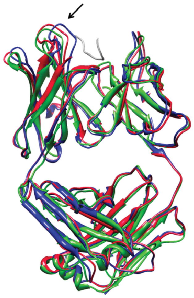
The FiberDock refinement result of test case number 9 (1GGI), HIV-1 neutralizing antibody in complex with its V3 loop peptide antigen, starting from the known binding orientation of the ligand (the antigen) and unbound conformation of the receptor (the antibody). The unbound structure of the receptor (the starting conformation of the refinement) is colored in blue and the bound structure of the receptor is in green. The bound ligand in the native orientation is presented in gray. The refined structure of the receptor, which was created by FiberDock, is in red. The refinement predicted accurately the loop movement in the binding site of the antibody that occurs during the interaction with the antigen (marked by an arrow). This image was produced using the UCSF Chimera package.⁴⁸

Figure 3.

The influence of the highest amplitude modes used by FiberDock to model the backbone movement of the antibody in test case number 9 (1GGI). The upper graph shows the lowest frequency mode, which describes a collective deformation of the protein (blue line). The bottom graph shows a higher frequency mode (number 16), which has the highest amplitude in the linear combination of modes used by FiberDock to model the backbone movement of the antibody (pink line). This mode describes local deformation of the flexible loops in the interface (residues 220–305, marked by an orange line). The dashed black line shows the distance between the positions of each residue in the bound and unbound conformation. On the right, the structure of the bound (blue) and unbound (green) conformations of the antibody are shown. The flexible region of the antibody is marked by an orange circle. The image of the structure was produced using the UCSF Chimera package.⁴⁸

Although the improvement in the IRMSD was modest in this experiment, FiberDock results achieved much better energy values. According to the last CAPRI Assessment Meeting,⁴⁹ one of the current major challenges in docking is ranking docking solutions and sorting out false positives. The energy value is a crucial factor in the final ranking. A relatively accurate model (with low IRMSD) which has a high energy value will not be ranked high among a group of docking solution candidates. Therefore, the improvement in the energy of the refined models is very important in the docking scheme.

Docking refinement starting from random orientations of the ligand around the native binding orientation

In this experiment, we used FiberDock for local-docking around the native binding orientation of the ligand. We created 500 random transformations of the ligand around the native orientation and refined each of them. To create the random transformations, we sampled the three translation variables (in X,Y,Z axes) from a Gaussian distribution with mean 0 Å and standard deviation 3 Å. The three rotation variables (along the X,Y,Z axes) were sampled from a Gaussian distribution with mean 0° and standard deviation 8°. These selected values of standard deviations are similar to the values used in the perturbation studies of Gray et al.³⁵ (standard deviation of 8° for rotation, 3 Å for translation along the line of protein centers, and 8 Å for translation in the two perpendicular directions). By applying these 500 transformations on the ligand, we created 500 starting docking models for refinement.

In almost all of the test cases, the FiberDock refinement protocol produced many more near-native results with low-energy values than the FireDock method. We defined a good solution as a solution in which the energy score is negative and the IRMSD is lower than 4 Å, which is an acceptable solution according to the CAPRI contest.⁴⁷ The number of good solutions of FireDock and Fiber-Dock, for each test case, is presented in Figure 4.

Figure 4.

Results of refining 500 random transformations of the ligand around the true binding orientation by using the two methods, FireDock with rigid backbone (cyan and blue bars) and FiberDock with flexible backbone (orange and red bars). The cyan and orange bars show the results of the experiment with both the receptors and the ligands in their unbound conformation (UU). The blue and red bars show the results of the experiment with unbound structures of the receptors and bound structures of the ligands (UB). The histogram shows the ratio of good solutions out of the 500 refined models. A good solution is defined as a solution in which the IRMSD is lower than 4 Å and the energy value is negative. The histogram is sorted according to the ratio of good solutions of FireDock with unbound structures of the receptors and bound structures of the ligands (FireDock-UB). For cases that are marked by stars (*), a structure of the ligand in its unbound conformation was not available.

In 17 of the 20 test cases, the number of good solutions was higher in the results of FiberDock when compared with FireDock, in both the unbound–unbound (UU) experiment and the unbound–bound (UB) experiment. In eight cases, this number was higher by more than 40% (in both experiments). These eight cases include six cases where the binding site of the receptor opens upon binding. In one case (1FIN), none of the methods produced any good solutions. This is the most difficult case in the data set, with recIRMSD of 6.08 Å.

Figure 5 shows the best IRMSD solution out of the group of good solutions (in the UU experiment) of two test case numbers 11 and 18. In both cases, the refinement correctly modeled backbone movements, which are necessary for solving steric clashes of the receptor and the ligand in near-native orientations. In case number 11 (1IBR), the refinement moved a loop that blocks the binding site in the unbound conformation, allowing the ligand to enter the binding site in a near-native orientation without any clashes and with a low energy value.

Figure 5.

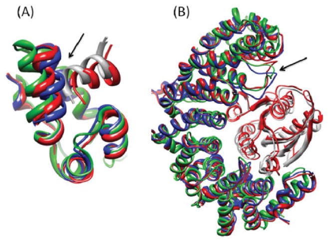
The best IRMSD solutions of the FiberDock method, out of the group of good solutions. (A) The solution of test case number 18 (HIV-1 capsid C-terminal domain with an inhibitor of particle assembly, pdb-id: 2BUO). (B) The solution of test case number 11 (complex of Ran with Importin beta, pdb-id: 1IBR). The unbound structures of the receptors (the starting conformations of the refinement) are colored in blue and the bound structures of the receptor are in green. The bound ligands in the native orientation are presented in gray. The refinement solutions, which were created by FiberDock, are in red. The refinement accurately predicted the backbone movements which the receptor undergoes during the interaction with the ligand. In both cases the refinement correctly modeled backbone movements which are necessary for resolving steric clashes of the receptor and the ligand in near-native orientations. The locations of these important backbone movements are marked by arrows. This image was produced using the UCSF Chimera package.⁴⁸

The refined structure of the receptor was created by a linear combination of both low- and high-frequency normal modes, described by the formula: $R^{\prime }=R+9.84V_1+4.31V_2-0.83V_3-10.63V_4-7.43V_5-1.84V_6-4.70V_7+9.21V_8-2.78V_{10}-5.10V_{11}-5.00V_{12}-3.93V13-1.16V_{15}+2.50V_{16}+1.78V_{17}-3.49V_{22}-0.78V_{23}-2.34V_{41}$, where R is the structure of the unbound receptor, V_i is the i^th normal mode, and R′ is the modeled structure of the receptor. The five normal modes that have the highest amplitude in this linear combination are mode numbers 1, 4, 5, 8, and 11. The influence of each normal mode on each residue is shown in Figure 6. The lower frequency modes (numbers 1, 4, and 5) describe a collective deformation of the protein, whereas the higher frequency modes (numbers 8 and 11) describe local deformation of the loop in the interface (residues 332–344). Figure 6 also shows the distance between the positions of each residue in the bound and unbound conformation. These distances have four high peaks (marked A–D in Figure 6). The highest peak (C) is between residues 288 and 316. However, these residues are located on the opposite side of the ligand, and their movement is not important for correct modeling of the interaction. The most important movement is of the interface loop (peak D), which is modeled by modes 8 and 11 during the backbone refinement of FiberDock.

Figure 6.

The influence of the highest amplitude modes used by FiberDock to model the backbone movement of the receptor in test case number 11 (1IBR). The upper graph shows the three low-frequency modes (1,4,5) which describe collective deformations of the protein. The two higher frequency modes (8,11), shown in the bottom graph, describe local deformation of the loop in the interface (residues 332–344). The dashed black line shows the distance between the positions of each residue in the bound and unbound conformation. These distances have four high peaks (marked A–D) in the most flexible positions. On the right, the structure of the bound (blue) and unbound (green) conformations are shown. The flexible regions, which correspond to the peaks, are marked by orange circles. The interface residues are marked by red lines in the x-axis. The image of the structure was produced using the UCSF Chimera package.⁴⁸

In case number 18 (2BUO), the refinement moved a helix and opened the binding site. Figure 5(A) clearly shows that the ligand in its native orientation has a major steric clash with the receptor in the unbound conformation. Therefore, without modeling the backbone movement of the receptor, a low-energy near-native solution cannot be achieved. In this case, the structure of the receptor was also created by a linear combination of both low- and high-frequency normal modes: R′ = R − 1.99V₁ − 0.36V₂ − 3.45V₃ + 4.22V₄ + 0.16V₉ + 3.08V₁₀ − 0.07V₁₄ − 2.18V₂₁ + 3.51V₂₃ + 2.58V₂₆.

Local docking by FiberDock produces more accurate results than RosettaDock

The local docking results of FiberDock were compared with the local docking results of RosettaDock3.0, which keeps the backbone rigid and models only side-chain flexibility. For both methods, we randomly sampled 500 rigid-body perturbations of the ligand, in the bound conformation, from a similar distribution (Gaussian distribution with standard deviation of 3 Å for translation and standard deviation of 8° for rotation). For each test case, we compared the accuracy of the lowest IRMSD result in the top 10 solutions (with the lowest energy) of the two methods. The comparison is detailed in Table III.

Table III.

Local Docking Results of FiberDock and RosettaDock

Complex ID	Best IRMSD in top 10
	FiberDock	RosettaDock3.0	ΔIRMSD*
1. 1A0O	1.8	3.11	−1.31
2. 1ACB	2.21	2.49	−0.28
3. 1AY7†	0.89	0.72	0.17
4. 1BTH	1.24	1.24	0.00
5. 1CGI	2.00	2.04	−0.04
6. 1DFJ†	1.11	5.80	−4.69
7. 1E6E	0.63	1.71	−1.08
8. 1FIN†	5.90	5.93	−0.03
9. 1GGI†	1.70	2.58	−1.88
10. 1GOT†	2.59	3.89	−1.3
11. 1IBR†	1.98	9.01	−7.03
12. 1OAZ	2.62	1.55	1.07
13. 1PXV	3.23	3.34	−0.11
14. 1T6G†	0.77	2.34	−1.57
15. 1TGS	1.38	1.31	0.07
16. 1WQ1	1.41	5.06	−3.65
17. 1ZHI	1.12	0.9	0.22
18. 2BUO†	3.62	4.24	−0.62
19. 2KAI	0.75	0.67	0.08
20. 3HHR†	1.89	4.30	−2.41

^*ΔIRMSD is the difference between the best IRMSD in the top 10 solutions of FiberDock and RosettaDock.

^†Cases where the conformation of the unbound receptor partially blocks the binding site of the ligand and the receptors undergoes an opening motion upon binding.

In 11 of the 20 test cases, FiberDock produced more accurate results than RosettaDock (with ΔIRMSD = IRMSD_FiberDock − IRMSD_RosettaDock < −0.2 Å). These cases include most of the test cases where the receptor undergoes an opening motion upon binding. Only in two cases RosettaDock produced better results (ΔIRMSD > 0.2 Å), and in seven cases, the accuracy of the results were about the same (−0.2 Å < ΔIRMSD < 0.2 Å). This comparison shows the ability of FiberDock in modeling opening motions of binding sites and its contribution in producing accurate models of protein–protein complexes.

Wang et al.²² have recently incorporated explicit backbone flexibility into RosettaDock. During each MC iteration of RosettaDock, a random backbone perturbation is performed together with a rigid-body perturbation. Although the method enables modeling full backbone flexibility for both proteins, in practice, this is extremely computationally demanding because of the high number of degrees of freedom. Therefore, it is feasible only for very small proteins or very subtle backbone perturbations. A more practical use of this method is to predefine the flexible segments of the protein (by a “fold tree”²²) and perturb backbone conformational changes only in these regions. This, however, requires prior knowledge of the flexible regions. FiberDock, on the other hand, minimizes the backbone conformation along few degrees of freedom, which are carefully picked by NMA. Therefore, the backbone refinement is much faster. In addition, as FiberDock considers both low- and high-frequency normal modes, both global and local conformational changes are modeled, and no prior knowledge of the flexible regions is required. By the time this article was written, backbone flexibility was not yet included in the latest RosettaDock release (version 3.0). Hence, we did not compare the performance of the backbone refinement of RosettaDock to FiberDock.

FiberDock improves the shape of energetic funnels around near-native results

The formation of energy funnels is known to be a relatively reliable indicator for identifying near-native models of protein–protein complexes among a group of solution candidates.^50,51 We used the 500 refined near-native complexes of FiberDock, FireDock, and RosettaDock, generated in the local docking experiments described earlier, to draw energy funnels around the native orientation of the ligands. In many cases, the shapes of the energetic funnels, which were created by FiberDock, were significantly better than the ones created by RosettaDock and FireDock. These funnels usually included many more near-native complex models and reached lower energy values. The energetic funnels of four of these cases (1CGI, 1IBR, 1T6G, 2BUO), using unbound receptors and bound ligands, are shown in Figure 7.

Figure 7.

Funnels created by the three refinement methods: RosettaDock, FireDock, and FiberDock, using unbound structure of the receptor and bound structure of the ligand. Each row compares the funnels created for a certain test case (pdb-id is specified on the left). The x-axis denotes the IRMSD of the refined complex, and the y-axis denotes its energy score value.

The improvement in the shape of the funnels generated by FiberDock when compared with FireDock, shown in Figure 7, is clearly due to the backbone refinement procedure, which is the only difference between the two methods. However, the figure also shows that FireDock generates better looking funnels when compared with RosettaDock, although both methods model side-chain flexibility by the same rotamer library and they both optimize the relative rigid-body orientation by a similar technique. There are two possible explanations for these differences in the created energy funnels: (1) The energy function of RosettaDock might be more sensitive to steric clashes than the energy function of FireDock. In these test cases, all of which include backbone conformational changes, most of the near-native (rigid backbone) results contain a certain amount of steric clashes. Energy functions that are too sensitive to clashes would not show a funnel-shaped energy landscape around the native ligand orientation. (2) The side-chain optimization technique is different in these two methods. FireDock optimizes the rotamers selection by the ILP approach, which guarantees to find the combination of rotamers that globally minimizes the repulsive vdW interface energy. RosettaDock, on the other hand, uses the heuristic MC technique for side-chain repacking. To fully understand the true reason for these differences in the shape of energy funnels, further research should be performed, which is out of the scope of this work.

Docking refinement starting from rigid-body docking candidates

In this experiment, we test the contribution of the backbone refinement procedure to the refinement and ranking of rigid-body docking solutions. For each test case, we identified the interacting amino acids (residues which contain an atom within 6 Å from the interacting protein). Then, we ran the PatchDock^43,44 method given the information on the location of the binding site.

Some of the proteins in our data set undergo significant conformational changes upon binding. Therefore, a completely blind rigid-docking run might not have had a near-native solution in its first 500 solution candidates. As we test the refinement and reranking abilities of our method, we used the binding site information, which is often known from experimental data.

The solutions of PatchDock are ranked by a shape complementarity score. We refined and reranked the best 500 solution candidates by FireDock and FiberDock and compared the results of the three methods (PatchDock, FireDock, and FiberDock). We performed this experiment on the unbound conformation of the receptors and the bound conformation of the ligands. The results are presented in Table IV.

Table IV.

Refinement of Right-Body Docking Solution Candidates (for Unbound Receptors and Bound Ligands)

Complex ID	PatchDock		FireDock			FiberDock
	First acceptablea	Acceptables in top 20b	First acceptablea	Original PatchDock resultc	Acceptables in top 20b	First Acceptablea	Original PatchDock resultc	Acceptables in top 20b
1A0O	1* (7.66, 3.79)	3†	7 (6.34, 2.30)	29 (9.20, 3.15)	3†	16 (5.25, 3.33)	108 (5.19, 3.26)	1
1ACB	3 (6.17, 3.12)	2	3 (8.24, 4.31)	259 (8.67, 4.37)	1	2* (6.84, 4.01)	42 (6.12, 3.56)	4†
1AY7	14 (9.78, 5.27)	3	5* (1.37, 0.77)	95 (4.19, 1.29)	5†	5* (1.37, 0.77)	95 (4.19, 1.29)	5†
1BTH	1* (12.10, 3.65)	1	2 (10.11, 3.28)	72 (11.47, 3.63)	2	1* (7.98, 1.97)	403 (14.80, 3.55)	5†
1CGI	2 (3.82, 2.31)	1	1* (2.82, 2.25)	2 (3.82, 2.31)	10†	1* (5.42, 2.72)	279 (7.50, 2.97)	9
1DFJ	1* (6.84, 2.76)	4	1* (5.55, 2.03)	2 (4.78, 2.33)	6†	1* (3.10. 1.53)	5 (4.28, 2.13)	6†
1E6E	None	0	474 (6.01, 3.32)	134 (10.20, 4.25)	0	2* (8.38, 3.44)	327 (20.64, 7.46)	2†
1FIN	None	0	None	None	0	None	None	0
1GGI	3 (6.06, 3.24)	6†	25 (6.83, 3.37)	3 (6.06, 3.24)	0	1* (12,39, 3.77)	281 (11.23, 3.29)	2
1GOT	None	0	None	None	0	None	None	0
1IBR	32 (6.99, 2.78)	0	2* (5.01, 2.50)	208 (6.38, 2.85)	1	2* (6.67, 2.61)	32 (6.99, 2.78)	3†
1OAZ	58 (18.47, 3.84)	0	9* (14.41, 3.27)	204 (15.05, 3.59)	1†	16 (14.41, 3.27)	204 (15.05, 3.59)	1†
1PXV	51 (8.54, 4.03)	0	17 (6.94, 3.49)	54 (5.78, 3.39)	1	1* (8.86, 4.51)	63 (9.86, 4.57)	2†
1T6G	4 (8.10, 1.75)	1	1* (6.83, 1.33)	129 (14.78, 3.08)	10	1* (9.61, 1.80)	70 (13.51, 2.33)	11†
1TGS	15 (2.69, 1.54)	1	1* (1.94, 1.43)	15 (2.69, 1.54)	10	1* (1.94, 1.43)	15 (2.69, 1.54)	11†
1WQ1	6* (2.24, 1.42)	1†	20 (5.64, 2.35)	82 (5.40, 2.17)	1†	29 (8.92, 4.44)	445 (7.18, 2.95)	0
1ZHI	134 (13.44, 2.81)	0	10 (7.52, 2.73)	311 (8.43, 3.03)	2	4* (7.18, 3.48)	311 (8.43, 3.03)	3†
2BUO	1* (9.38, 5.39)	9†	3 (5.05, 3.91)	32 (4.87, 3.98)	3	12 (6.3, 4.61)	203 (8.3, 4.71))	2
2KAI	17 (12.46, 3.23)	1	1* (1.94, 0.84)	257 (1.11, 0.77)	3†	1* (2.18, 0.94)	257 (1.11, 0.77)	2
3HHR	214* (11.61, 3.27)	0	497 (9.19, 5.51)	420 (9.17, 4.59)	0	214* (13.59, 3.95)	261 (15.38, 3.77)	0
wins‡	6	4	8		7	14		11

^aThe rank of the first acceptable solution. The RMSD and the IRMSD of this solution are in brackets in the corresponding order.

^bThe number of acceptable solutions in the top 20 solutions.

^cThe rank of the original PatchDock solution of the first acceptable solution, before the refinement, according to the shape complementarity score of PatchDock. The RMSD and the IRMSD of this solution are in brackets in the corresponding order.

^*The best rank of the first acceptable solution among the three methods (PatchDock, FireDock, and FiberDock).

^†The highest number of acceptable solutions in the top 20 solutions of the three methods.

^‡The wins row summarizes the number of cases that a method achieved the best rank of the first acceptable solution or the highest number of acceptable solutions in the top 20 solutions.

Table IV shows the rank of the first acceptable solution (IRMSD < 4.0 Å or RMSD < 10.0 Å) and the number of acceptable solutions in the top 20 solutions for each of the methods. The results show a gradual improvement in these criteria. The rank of the first acceptable solution was the best in the results of PatchDock in 6 cases and in the results of FireDock and FiberDock in 8 and 14 cases, respectively. The number of acceptable solutions in the top 20 solutions also increased gradually. In 4 cases, this number was the highest for PatchDock results, and in 7 and 11 cases, it was the highest for the results of Fire-Dock and FiberDock, respectively. These results show that backbone refinement can significantly improve the ranking of near-native docking solutions, as it often solves steric clashes between the interacting proteins that prevent the docking solution from getting a low energy value and good ranking (shown earlier).

In case number 14 (1T6G), the first solution of Fiber-Dock was of medium accuracy according to CAPRI criteria. However, the second solution was highly accurate, with IRMSD of 0.92 Å and RMSD of 3.04 Å (not shown in the table). By examining the structure of the refined model, depicted in Figure 8, one can see that FiberDock automatically identified the single loop that slightly moves during the interaction to open the binding site and enable the ligand to enter it in the correct orientation. FiberDock moved this flexible loop in the right direction and kept the other parts of the protein rigid.

Figure 8.

FiberDock’s predicted model of test case number 14 (complex of Endo-1,4-beta-xylanase I and xylanase inhibitor, pdb-id: 1T6G). This model was ranked in second place after refining end reranking the 500 top solutions of PatchDock. The unbound structure of the receptor (the starting conformations of the refinement) is colored in blue and the bound structure of the receptor is in green. The bound ligand in the native orientation is presented in gray. The refinement solution, which was created by FiberDock, is in red. The refinement accurately predicted the loop movement that occurs in the receptor during the interaction with the ligand. This image was produced using the UCSF Chimera package.⁴⁸

The table also provides details relating to the original PatchDock solution of the first acceptable solution of FireDock and FiberDock before the refinement. The refinement by both FireDock and FiberDock significantly improves the ranking and the accuracy of the rigid-docking results. For example, in case number 4 (1BTH), an inaccurate PatchDock solution with RMSD of 14.8 Å and IRMSD of 3.55 Å which was ranked in place 403, was refined by FiberDock to a more accurate model (RMSD of 7.98 Å and IRMSD of 1.97 Å) which was ranked in first place by its energy function. The refinement by Fire-Dock, on the other hand, resulted in a worse model (RMSD of 18.9 Å and IRMSD of 4.64 Å). In this case, FiberDock hardly changed the backbone conformation of the receptor (RMSD of 0.15 Å between the modeled and the unbound conformation of the receptor). However, this case shows that even a slight movement of the backbone, which resolve steric clashes, may enable the rigid-body optimization stage to converge to a near-native position. The results of the refinement by the two methods are shown in Figure 9.

Figure 9.

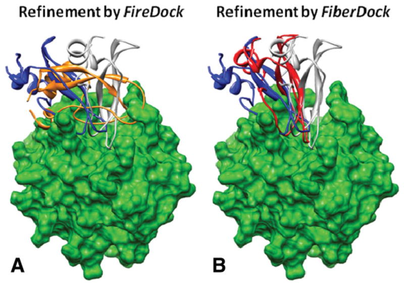
Refinement of a rigid-docking solution of case number 5 (Thrombin complexed with bovine pancreatic trypsin inhibitor, pdb-id: 1BTH) by FireDock (A) and FiberDock (B). The receptor in its bound conformation is presented in green. The ligand in the native orientation is colored in gray. The original rigid-docking solution (generated by PatchDock), on which the refinement was applied, is colored in blue. The position of the ligand after the refinement by FireDock is presented in orange, and the position of the ligand after the refinement by FiberDock is in red. This case shows a drastic improvement of the docking solution due to the flexible refinement by FiberDock. This image was produced using the UCSF Chimera package.⁴⁸

DISCUSSION AND CONCLUSIONS

The structure prediction of protein–protein complexes usually consists of two major stages: soft rigid-docking, which allows a certain amount of steric clashes, followed by flexible refinement. CAPRI challenges^45–47 showed that in many cases the rigid-docking stage succeeds in producing a near-native result. However, this result often contains steric clashes, and therefore it is ranked low in the list of solution candidates. The goal of the flexible refinement stage is to refine thousands of rigid-docking solutions, resolve their steric clashes, and evaluate their binding energies which are used for reranking. This is an extremely important stage that is necessary for identifying near-native models among a group of docking candidates and to create even more accurate models which will help scientists study and understand the chemical mechanism of molecular complexes.

In this article, we presented a new method for flexible refinement of docking solution candidates, called Fiber-Dock. The method models both side-chain and backbone flexibility and performs rigid body optimization on the ligand orientation. The refinement algorithm mimics an induced-fit process. The backbone and side-chain movements are modeled according to the vdW forces between the receptor and ligand. The backbone movements are modeled using the NMA approach. Unlike previous methods,^24,25 FiberDock uses both low- and high-frequency normal modes, and therefore it is able to model both global and local conformational changes such as opening of binding sites and loop movement. The results show that the method successfully models backbone movements that occur during molecular interactions. The inclusion of the backbone refinement procedure in the refinement process was shown to improve both the accuracy and the ranking of near-native docking solution candidates. Moreover, accounting for backbone flexibility improves the shape of energy funnels around the native docking orientation. These energy funnels can assist in identifying near-native solutions among a group of solution candidates.

Modeling backbone flexibility is necessary not only in cases where the proteins change conformation upon binding but also in cases where the 3D structures of the interacting proteins are not available and models are used. Backbone refinement might be able to deal with the inaccuracy of the models in these cases. In addition, we expect FiberDock to be helpful in predicting antibody–antigen complexes. Docking in this field is known to be difficult due to the flexible CDR loops. Our data-set contained a single antibody–antigen case (HIV-1 neutralizing antibody in complex with its V3 loop peptide antigen, pdb-id: 1GGI) in which a CDR loop moves upon binding. FiberDock improves the refinement of this complex, when compared with FireDock (see Fig. 2). We plan to further investigate the performance of the FiberDock method on antibody–antigen complexes.

Currently, the FiberDock method is particularly helpful in cases where the receptor undergoes an opening conformational change induced by steric clashes. In general, opening movements are easier to handle in docking as modeling the precise alternate conformation is not essential for generating an accurate model of the molecular complex with low-energy score. The current version of FiberDock will not model movements induced by attractive forces, such as closing of a binding site around the ligand, as the correlation measurement, used for selecting the relevant modes, uses only the repVdW forces. In the future, we plan to incorporate additional chemical forces (e.g., attractive vdW forces, electrostatic forces, and hydrogen bonds) in the normal modes selection step of the backbone refinement procedure. In addition, we plan to simultaneously model backbone flexibility of both the receptor and the ligand. This can be achieved by a minor modification in the backbone refinement procedure, by choosing the most relevant normal mode among a set of both the receptor’s and ligand’s normal modes.

FiberDock deals with relatively subtle backbone conformational changes that occur upon binding. It achieves good refinement results in cases where the receptor interface RMSD (recIRMSD) is below 5 Å. In cases with larger conformational changes, an initial near-native rigid-docking solution cannot be generated, and therefore other approaches should be considered. An analysis should be performed prior to the docking to assess the level of flexibility of the interacting proteins. One of the common types of backbone flexibility is a hinge bending motion. Hinge locations can be predicted by the Hinge-Prot method,⁵² which analyzes the two lowest frequency normal modes. Hinge motions usually result in a large conformational change that prevents any rigid-docking method from generating a near-native model. In these cases, one can perform flexible docking by the FlexDock method.⁵³ This method divides the flexible protein into its rigid parts, dock each part separately and then assemble the partial docking solutions into consistent flexible docking models. Hinge-bending motions are often coupled with other types of backbone flexibility (e.g., flexible loops). These can be handled by refining Flex-Dock solutions using the FiberDock method.

In other cases where a high level of backbone flexibility is predicted, cross-docking of pre-generated conformations should be performed, followed by flexible refinement of the solutions. This will mimic both the conformational selection process and the induced-fit process. A similar approach was recently tested by Chadhury and Gray¹⁴ with promising results. However, cross-docking might produce many more solutions with good energy values. Therefore the identification of near-native solutions among them will be more difficult. To correctly rank the solution candidates, a more accurate and robust energy function should be developed, and energy funnels should be searched around the lowest energy solutions.

References

- 1.Ma B, Kumar S, Tsai CJ, Nussinov R. Folding funnels and binding mechanisms. Protein Eng. 1999;12:713–720. doi: 10.1093/protein/12.9.713. [DOI] [PubMed] [Google Scholar]
- 2.Kumar S, Ma B, Tsai CJ, Sinha N, Nussinov R. Folding and binding cascades: dynamic landscapes and population shifts. Protein Sci. 2000;9:10–19. doi: 10.1110/ps.9.1.10. [DOI] [PMC free article] [PubMed] [Google Scholar]
- 3.Tsai CJ, Ma B, Sham YY, Kumar S, Nussinov R. Structured disorder and conformational selection. Proteins. 2001;44:418–427. doi: 10.1002/prot.1107. [DOI] [PubMed] [Google Scholar]
- 4.James LC, Roversi P, Tawfik DS. Antibody multispecificity mediated by conformational diversity. Science. 2003;299:1362–1367. doi: 10.1126/science.1079731. [DOI] [PubMed] [Google Scholar]
- 5.Ma B, Shatsky M, Wolfson HJ, Nussinov R. Multiple diverse ligands binding at a single protein site: a matter of pre-existing populations. Protein Sci. 2002;11:184–197. doi: 10.1110/ps.21302. [DOI] [PMC free article] [PubMed] [Google Scholar]
- 6.Koshland DE. Application of a theory of enzyme specificity to protein synthesis. Proc Natl Acad Sci USA. 1958;44:98–104. doi: 10.1073/pnas.44.2.98. [DOI] [PMC free article] [PubMed] [Google Scholar]
- 7.Goh CS, Milburn D, Gerstein M. Conformational changes associated with protein–protein interactions. Curr Opin Chem Biol. 2004;14:1–6. doi: 10.1016/j.sbi.2004.01.005. [DOI] [PubMed] [Google Scholar]
- 8.Grunberg R, Leckner J, Nilges M. Complementarity of structure ensembles in protein–protein binding. Struct. 2004;12:2125–2136. doi: 10.1016/j.str.2004.09.014. [DOI] [PubMed] [Google Scholar]
- 9.Boehr DD, Nussinov R, Wright PE. The role of dynamic conformational ensembles in biomolecular recognition. Nat Chem Biol. 2009;5:789–796. doi: 10.1038/nchembio.232. [DOI] [PMC free article] [PubMed] [Google Scholar]
- 10.Andrusier N, Mashiach E, Nussinov R, Wolfson HJ. Principles of flexible protein–protein docking. Proteins. 2008;73:271–289. doi: 10.1002/prot.22170. [DOI] [PMC free article] [PubMed] [Google Scholar]
- 11.Smith GR, Sternberg MJE, Bates PA. The relationship between the flexibility of proteins and their conformational states on forming protein–protein complexes with application to protein–protein docking. J mol Biol. 2005;347:1077–1101. doi: 10.1016/j.jmb.2005.01.058. [DOI] [PubMed] [Google Scholar]
- 12.Mustard D, Ritchie DH. Docking essential dynamics eigenstructures. Proteins. 2005;60:269–274. doi: 10.1002/prot.20569. [DOI] [PubMed] [Google Scholar]
- 13.Król M, Chaleil RA, Tournier AL, Bates PA. Implicit flexibility in protein docking: cross-docking and local refinement. Proteins. 2007;69:750–757. doi: 10.1002/prot.21698. [DOI] [PubMed] [Google Scholar]
- 14.Chaudhury S, Gray JJ. Conformer selection and induced fit in flexible backbone protein–protein docking using computational and NMR ensembles. J Mol Biol. 2008;381:1068–1087. doi: 10.1016/j.jmb.2008.05.042. [DOI] [PMC free article] [PubMed] [Google Scholar]
- 15.Bastard K, Thureau A, Lavery R, Prevost C. Docking macromolecules with flexible segments. J Comput Chem. 2003;24:1910–1920. doi: 10.1002/jcc.10329. [DOI] [PubMed] [Google Scholar]
- 16.Bastard K, Prevost C, Zacharias M. Accounting for loop flexibility during protein–protein docking. Proteins. 2006;62:956–969. doi: 10.1002/prot.20770. [DOI] [PubMed] [Google Scholar]
- 17.Dominguez C, Boelens R, Bonvin A. HADDOCK: a protein-protein docking approach based on biochemical or biophysical information. J Amer Chem Soc. 2003;125:1731–1737. doi: 10.1021/ja026939x. [DOI] [PubMed] [Google Scholar]
- 18.Fitzjohn PW, Bates PA. Guided docking: first step to locate potential binding sites. Proteins. 2003;52:28–32. doi: 10.1002/prot.10380. [DOI] [PubMed] [Google Scholar]
- 19.Smith GR, Fitzjohn PW, Page CS, Bates PA. Incorporation of flexibility into rigid-body docking: applications in rounds 3–5 of CAPRI. Proteins. 2005;60:263–268. doi: 10.1002/prot.20568. [DOI] [PubMed] [Google Scholar]
- 20.Krol M, Tournier AL, Bates PA. Flexible relaxation of rigid-body docking solutions. Proteins. 2007;68:159–169. doi: 10.1002/prot.21391. [DOI] [PubMed] [Google Scholar]
- 21.de Vries SJ, van Dijk AD, Krzeminski M, van Dijk M, Thureau A, Hsu V, Wassenaar T, Bonvin AM. HADDOCK versus HADDOCK: new features and performance of HADDOCK2. 0 on the CAPRI targets. Proteins. 2007;69:726–733. doi: 10.1002/prot.21723. [DOI] [PubMed] [Google Scholar]
- 22.Wang C, Bradley P, Baker D. Protein–protein docking with backbone flexibility. J Mol Biol. 2007;373:505–515. doi: 10.1016/j.jmb.2007.07.050. [DOI] [PubMed] [Google Scholar]
- 23.Chaudhury S, Sircar A, Sivasubramanian A, Berrondo M, Gray JJ. Incorporating biochemical information and backbone flexibility in RosettaDock for CAPRI rounds 6–12. Proteins. 2007;69:793–800. doi: 10.1002/prot.21731. [DOI] [PubMed] [Google Scholar]
- 24.Lindahl E, Delarue M. Refinement of docked protein–ligand and protein–DNA structures using low frequency normal mode amplitude optimization. Nucleic Acids Res. 2005;33:4496–4506. doi: 10.1093/nar/gki730. [DOI] [PMC free article] [PubMed] [Google Scholar]
- 25.May A, Zacharias M. Energy minimization in low-frequency normal modes to efficiently allow for global flexibility during systematic protein–protein docking. Proteins. 2008;70:794–809. doi: 10.1002/prot.21579. [DOI] [PubMed] [Google Scholar]
- 26.Tirion MM. Large amplitude elastic motions in proteins from a single-parameter, atomic analysis. Phys Rev Lett. 1996;77:1905–1908. doi: 10.1103/PhysRevLett.77.1905. [DOI] [PubMed] [Google Scholar]
- 27.Hinsen K. Analysis of domain motions by approximate normal mode calculations. Proteins. 1998;33:417–429. doi: 10.1002/(sici)1097-0134(19981115)33:3<417::aid-prot10>3.0.co;2-8. [DOI] [PubMed] [Google Scholar]
- 28.Ma J. New advances in normal mode analysis of supermolecular complexes and applications to structural refinement. Curr Protein Pept Sci. 2004;5:119–123. doi: 10.2174/1389203043486892. [DOI] [PMC free article] [PubMed] [Google Scholar]
- 29.Tama F, Sanejouand YH. Conformational change of proteins arising from normal mode calculations. Protein Eng. 2001;14:1–6. doi: 10.1093/protein/14.1.1. [DOI] [PubMed] [Google Scholar]
- 30.May A, Zacharias M. Accounting for global protein deformability during protein–protein and protein–ligand docking. Biochim Bio-phys Acta. 2005;1754:225–231. doi: 10.1016/j.bbapap.2005.07.045. [DOI] [PubMed] [Google Scholar]
- 31.Petrone P, Pande VS. Can conformational change be described by only a few normal modes? Biophys J. 2006;90:1583–1593. doi: 10.1529/biophysj.105.070045. [DOI] [PMC free article] [PubMed] [Google Scholar]
- 32.Dobbins SE, Lesk VI, Sternberg MJ. Insights into protein flexibility: the relationship between normal modes and conformational change upon protein-protein docking. Proc Natl Acad Sci USA. 2008;105:10390–10395. doi: 10.1073/pnas.0802496105. [DOI] [PMC free article] [PubMed] [Google Scholar]
- 33.Cavasotto CN, Kovacs JA, Abagyan RA. Representing receptor flexibility in ligand docking through relevant normal modes. J Am Chem Soc. 2005;127:9632–9640. doi: 10.1021/ja042260c. [DOI] [PubMed] [Google Scholar]
- 34.Andrusier N, Nussinov R, Wolfson HJ. FireDock: fast interaction refinement in molecular docking. Proteins. 2007;69:139–159. doi: 10.1002/prot.21495. [DOI] [PubMed] [Google Scholar]
- 35.Gray JJ, Moughon S, Schueler-Furman O, Kuhlman B, Rohl CA, Baker D. Protein-protein docking with simultaneous optimization of rigid-body displacement and side-chain conformations. J Mol Biol. 2003;331:281–299. doi: 10.1016/s0022-2836(03)00670-3. [DOI] [PubMed] [Google Scholar]
- 36.Eriksson O. Side chain-positioning as an integer programming problem. Lect Notes in Comput Sci. 2001;2149:128–141. [Google Scholar]
- 37.Broyden CG. The convergence of a class of double-rank minimization algorithms. J Inst Math Appl. 1970;6:76–90. [Google Scholar]
- 38.Fletcher R. A new approach to variable metric algorithms. Comput J. 1970;13:317–322. [Google Scholar]
- 39.Atilgan AR, Durell SR, Jernigan RL, Demirel MC, Keskin O, Bahar I. Anisotropy of fluctuation dynamics of proteins with an elastic network model. Biophys J. 2001;80:505–515. doi: 10.1016/S0006-3495(01)76033-X. [DOI] [PMC free article] [PubMed] [Google Scholar]
- 40.MacKerell AD, Jr, Bashford D, Bellott M, Dunbrack RL, Jr, Evanseck JD, Field MJ, Fischer S, Gao J, Guo H, Ha S, Joseph-McCarthy D, Kuchnir L, Kuczera K, Lau FTK, Mattos C, Michnick S, Ngo T, Nguyen DT, Prodhom B, Reiher WE, III, Roux B, Schlenkrich M, Smith JC, Stote R, Straub J, Watanabe M, Wiórkiewicz-Kuczera J, Yin D, Karplus M. All-atom empirical potential for molecular modeling and dynamics studies of proteins. J Phys Chem. 1998;102:3586–3616. doi: 10.1021/jp973084f. [DOI] [PubMed] [Google Scholar]
- 41.Dunbrack RL, Jr, Canutescu AA. Cyclic coordinate descent: a robotics algorithm for protein loop closure. Protein Sci. 2003;12:963–972. doi: 10.1110/ps.0242703. [DOI] [PMC free article] [PubMed] [Google Scholar]
- 42.Mendez R, Leplae R, De Maria L, Wodak SJ. Assessment of blind predictions of protein-protein interactions: current status of docking methods. Proteins. 2003;52:51–67. doi: 10.1002/prot.10393. [DOI] [PubMed] [Google Scholar]
- 43.Duhovny D, Nussinov R, Wolfson HJ. In: Guigo R, Gusfield D, editors. Efficient unbound docking of rigid molecules; Proceedings of the 2’nd Workshop on Algorithms in Bioinformatics (WABI); Rome, Italy. Springer Verlag; 2002. pp. 185–200. [Google Scholar]
- 44.Schneidman-Duhovny D, Inbar Y, Nussinov R, Wolfson HJ. Patch-dock and symmdock: servers for rigid and symmetric docking. Nucleic Acids Res. 2005;33:W363–W367. doi: 10.1093/nar/gki481. [DOI] [PMC free article] [PubMed] [Google Scholar]
- 45.Lensink MF, Wodak SJ, Mendez R. Docking and scoring protein complexes: CAPRI 3rd edition. Proteins. 2007;69:704–718. doi: 10.1002/prot.21804. [DOI] [PubMed] [Google Scholar]
- 46.Mendez R, Leplae R, Lensink MF, Wodak SJ. Assessment of CAPRI predictions in rounds 3–5 shows progress in docking procedures. Proteins. 2005;60:150–169. doi: 10.1002/prot.20551. [DOI] [PubMed] [Google Scholar]
- 47.Schneidman-Duhovny D, Inbar Y, Polak V, Shatsky M, Halperin I, Benyamini H, Barzilai A, Dror O, Haspel N, Nussinov R, Wolfson HJ. Taking geometry to its edge: fast unbound rigid (and hinge-bent) docking. Proteins. 2003;52:107–112. doi: 10.1002/prot.10397. [DOI] [PubMed] [Google Scholar]
- 48.Pettersen EF, Goddard TD, Huang CC, Couch GS, Greenblatt DM, Meng EC, Ferrin TE. UCSF Chimera — a visualization system for exploratory research and analysis. J Comput Chem. 2004;25:1605–1612. doi: 10.1002/jcc.20084. [DOI] [PubMed] [Google Scholar]
- 49.Janin J, Wodak S. The third CAPRI assessment meeting, Toronto, Canada, April 20–21, 2007. Structure. 2007;15:755–759. doi: 10.1016/j.str.2007.06.007. [DOI] [PubMed] [Google Scholar]
- 50.Schueler-Furman O, Wang C, Baker D. Progress in protein-protein docking: atomic resolution predictions in the CAPRI experiment using RosettaDock with an improved treatment of side-chain flexibility. Proteins. 2005;60:187–194. doi: 10.1002/prot.20556. [DOI] [PubMed] [Google Scholar]
- 51.Schueler-Furman O, Wang C, Bradley P, Misura K, Baker D. Progress in modeling of protein structures and interactions. Science. 2005;310:638–642. doi: 10.1126/science.1112160. [DOI] [PubMed] [Google Scholar]
- 52.Emekli U, Schneidman-Duhovny D, Wolfson HJ, Nussinov R, Haliloglu T. HingeProt: automated prediction of hinges in protein structures. Proteins. 2008;70:1219–1227. doi: 10.1002/prot.21613. [DOI] [PubMed] [Google Scholar]
- 53.Schneidman-Duhovny D, Nussinov R, Wolfson HJ. Automatic prediction of protein interactions with large scale motion. Proteins. 2007;69:764–773. doi: 10.1002/prot.21759. [DOI] [PubMed] [Google Scholar]