Iron stable isotopes track pelagic iron cycling during a subtropical phytoplankton bloom

Significance

The supply and bioavailability of dissolved iron sets the magnitude of surface productivity for approximately 40% of the global ocean; however, our knowledge of how it is transferred between chemical states and pools is poorly constrained. Here we utilize the isotopic composition of dissolved and particulate iron to fingerprint its transformation in the surface ocean by abiotic and biotic processes. Photochemical and biological reduction and dissolution of particulate iron in the surface ocean appear to be key processes in regulating its supply and bioavailability to marine biota. Iron isotopes offer a new window into our understanding of the internal cycling of Fe, thereby allowing us to follow its biogeochemical transformations in the surface ocean.

Abstract

The supply and bioavailability of dissolved iron sets the magnitude of surface productivity for ∼40% of the global ocean. The redox state, organic complexation, and phase (dissolved versus particulate) of iron are key determinants of iron bioavailability in the marine realm, although the mechanisms facilitating exchange between iron species (inorganic and organic) and phases are poorly constrained. Here we use the isotope fingerprint of dissolved and particulate iron to reveal distinct isotopic signatures for biological uptake of iron during a GEOTRACES process study focused on a temperate spring phytoplankton bloom in subtropical waters. At the onset of the bloom, dissolved iron within the mixed layer was isotopically light relative to particulate iron. The isotopically light dissolved iron pool likely results from the reduction of particulate iron via photochemical and (to a lesser extent) biologically mediated reduction processes. As the bloom develops, dissolved iron within the surface mixed layer becomes isotopically heavy, reflecting the dominance of biological processing of iron as it is removed from solution, while scavenging appears to play a minor role. As stable isotopes have shown for major elements like nitrogen, iron isotopes offer a new window into our understanding of the biogeochemical cycling of iron, thereby allowing us to disentangle a suite of concurrent biotic and abiotic transformations of this key biolimiting element.

Springtime phytoplankton blooms are major contributors to the drawdown of carbon dioxide (CO₂) from the atmosphere and its sequestration into the ocean’s interior (1, 2). In the context of the ocean’s iron (Fe) biogeochemical cycle, spring blooms represent a transition from early season production, fueled largely by new Fe from underlying waters or lateral supply (3), to postbloom conditions where primary production is mainly (i.e., ∼90%) supported by an efficient Fe recycling loop between biogenic particulates and the dissolved Fe pool (3). Photochemical reduction and biological processing of inorganic, complexed, and particulate Fe significantly enhances Fe bioavailability (4–7); however, our understanding of the mechanisms, timing, and rates of Fe exchange between pools (dissolved, lithogenic, and biogenic) and redox species (Fe^II and Fe^III) during the onset and development of a phytoplankton bloom is limited. Indeed, the transient nature of many of these processes makes it difficult to quantify their influence on the biogeochemical cycling of Fe.

Iron isotope ratios (⁵⁶Fe/⁵⁴Fe) are a promising tool because isotope fractionation can occur upon transformation of Fe redox species (8), particulate dissolution (9), scavenging (10), precipitation (11), and biological uptake by phytoplankton (12). To date, a limited number of open ocean Fe isotope studies have been published (10, 12–14), with few combining both dissolved and particulate data to trace exchanges between various Fe pools. Here, we present Fe isotope data from two GEOTRACES (www.geotraces.org) process voyages (2008 and 2012) designed to study temporal changes in the biogeochemical cycling of Fe at the same locality in subtropical waters (38°S−39°S, 178°W−180°W) within the mesoscale eddy field east of New Zealand (3). We first present in situ results for dissolved and particulate Fe (DFe and PFe) cycling during the annual spring bloom, followed by the findings from a shipboard 700-L mesocosm incubation experiment, and then a conceptual model outlining the key chemical and biological processes involved in Fe isotope fractionation.

Results and Discussion

Across the two voyages, we identified three distinct stages associated with the progression of the annual spring bloom. Stage I is characterized by low Net Primary Productivity (NPP) (1.54 µmol C⋅L⁻¹⋅d⁻¹), low chlorophyll a (Chl) concentrations, low biomass (Fig. 1 and Fig. S1), and relatively homogenous nitrate and DFe profiles between 0 m and 250 m (Fig. 2A). This is indicative of a system that has been reset by turbulent mixing and convective overturning during winter (15) and primed, environmentally, for phytoplankton to bloom. Stage II is characterized by the initial development of a diatom-dominated bloom, increasing rates of NPP (6.15 µmol C⋅L⁻¹⋅d⁻¹) and phytoplankton and grazer biomass (Fig. 1 and Fig. S1), resulting in partial drawdown of nitrate and DFe within the mixed layer (Figs. 1 and 2B). Stage III is characterized by elevated NPP (10.7 µmol C⋅L⁻¹⋅d⁻¹), higher Chl concentrations/biomass (Fig. S1) and a corresponding biological depletion of nitrate and DFe within and immediately below the mixed layer (Figs. 1 and 2C and Fig. S1) (3, 16).

Fig. 1.

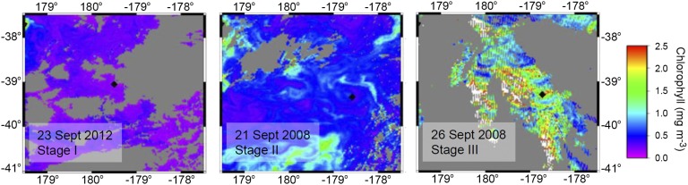
Satellite-derived chlorophyll concentrations for stages I, II, and III of the subtropical spring phytoplankton bloom. Diamond represents the sampling site. Gray areas represent cloud cover during the satellite pass-over. MODIS Aqua satellite data obtained from ERDDAP and plotted using Generic Mapping Tools (46).

Fig. 2.

DFe and δ⁵⁶Fe depth profiles. (A−C) Depth profiles of DFe and dissolved nitrate concentration across the three stages of the annual spring phytoplankton bloom. (D−F) The δ⁵⁶Fe results for dissolved, suspended (diamonds), and sinking particulates (upside-down triangles) across the three stages of the phytoplankton bloom. Error bars represent either 2 SDs for multiple sample extraction and isotope separations or 2 SEs of instrument precision for a single sample extraction and isotope separation.

A time-dependent change in the δ⁵⁶Fe composition of DFe and PFe is observed across stages I to III (Fig. 2 and Fig. S2). During stage I, the δ⁵⁶Fe composition of DFe and PFe within the euphotic zone was different, with lighter δ⁵⁶Fe values for DFe (Δ⁵⁶Fe_PFe-DFe = 0.28‰) relative to PFe (Fig. 2D). The dissolved δ⁵⁶Fe composition varied vertically whereby δ⁵⁶Fe values increased with depth (100–300 m), even though nitrate and the DFe profiles were homogenous (5.10 ± 0.19 µmol⋅L⁻¹ and 0.38 ± 0.02 nmol⋅kg⁻¹, respectively). At 300 m, the δ⁵⁶Fe composition of DFe and PFe was isotopically the same (0.04 ± 0.09‰ and 0.08 ± 0.01‰, respectively) and consistent with an inferred lithogenic provenance of coastally derived particulates (Fig. 2D and Fig. S2) (3, 12, 16, 17).

During stage I, there are two candidate processes that could lead to an isotopically light DFe pool within the euphotic zone: photochemical and biological reduction of PFe, the latter via acidic phagocytosis upon ingestion by protozoan grazers (18–20). The key process required for δ⁵⁶Fe fractionation is the reduction of Fe^III to Fe^II and its subsequent release into solution; δ⁵⁶Fe fractionation associated with proton-promoted dissolution of lithogenic Fe (e.g., goethite and hematite), as might occur in the digestive gut of grazers, is likely to be less (9, 21) compared with δ⁵⁶Fe fractionation associated with photochemical reduction of lithogenic Fe. It should also be noted that acidic and enzymatic digestion of PFe by grazers may also promote Fe reduction and solubilization (20), but it is usually followed by exposure to alkaline conditions, which leads to reoxidization before egestion (20). If a portion of this reduced, isotopically light Fe is taken up by the grazer, then this would lead to an isotopically heavier Fe composition of the remaining Fe pool upon reoxidation and loss via egestion. At this stage, we cannot fully disentangle the contributions of these two processes (photochemical versus grazer-mediated biological processing of lithogenic Fe) to the isotopically light dissolved Fe pool, but note from the information available that the photochemical reduction rate is likely to be two to three times higher than that of grazer-mediated Fe processing during stage I when grazer biomass and bacterial abundance were low (Table S1 and Fig. S1). Clearly, though, more work will be needed to distinguish between photochemical and biological effects on particulate iron dissolution and isotopic fractionation. These multiple lines of evidence (relationship between DFe and PFe, and isotopic signatures with depth) and, in particular, the low dissolved δ⁵⁶Fe values within the euphotic zone are consistent with the release of isotopically light Fe from lithogenic particulate material (22–25).

During the bloom onset (stage II), the δ⁵⁶Fe compositions of DFe and PFe within the mixed layer are the same within error (Δδ⁵⁶Fe_PFe-DFe = 0.05‰), indicating a biological influence on δ⁵⁶Fe fractionation (Fig. 2E). This is evident in size-fractionated plankton samples (0.2–20 µm and >20 µm) within the mixed layer, with the 0.2- to 20-µm size fraction being 0.15‰ lighter than the >20-µm size fraction (Fig. 3A). Pools of Fe associated with small phytoplankton are known to turn over on a timescale of hours (26); thus δ⁵⁶Fe fractionation in the 0.2- to 20-µm size fraction likely reflects fractionation associated with the rapid recycling of Fe between the DFe pool and biogenic components within the PFe pool. In addition, small (e.g., Synechococcus) and large phytoplankton (e.g., the diatom Asterionellopsis glacialis) may also fractionate δ⁵⁶Fe to differing degrees, although we did not see δ⁵⁶Fe fractionation between differing size classes in our mesocosm experiment (see below). Below the mixed layer, the δ⁵⁶Fe composition of DFe is lighter than PFe (Δ⁵⁶Fe_PFe-DFe = ∼0.2‰ at 100 m) (Fig. 2E), which is still characteristic of a system reset by winter mixing (15), even though DFe levels are ∼0.1 nmol⋅kg⁻¹ lower than during stage I.

Fig. 3.

Size-fractionated PFe and δ⁵⁶Fe depth profiles. (A) Depth profiles of size-fractionated (0.2–20 µm and >20 µm) PFe concentration and δ⁵⁶Fe. (B) PFe isotope versus Fe:Al ratio for suspended particulate matter across stages I to III along with the percentage of biogenic Fe for PFe. The percentage of biogenic Fe is iron is based on excess PFe relative to the lithogenic Fe:Al ratio of 0.18 (16). Error bars are the same as in Fig. 2.

At the peak of the bloom (stage III), the δ⁵⁶Fe composition of DFe within the mixed layer is heavier than the δ⁵⁶Fe composition of particulate material (Δ⁵⁶Fe_PFe-DFe = −0.26‰), consistent with isotope fractionation during biological uptake (Fig. 2F). Below the mixed layer, the δ⁵⁶Fe composition of DFe is also heavier than PFe and is linked to the depletion of DFe (Fig. 2C); the concentration of DFe at 100 m is ∼0.22 nmol⋅kg⁻¹ lower than during bloom stage I.

The overall change in Δ⁵⁶Fe_PFe-DFe across bloom stages I to III is −0.54‰ and is indicative of δ⁵⁶Fe fractionation mainly associated with DFe uptake by small phytoplankton (12). The changes observed in the δ⁵⁶Fe composition of DFe and PFe during the evolution of the bloom are supported by changes in the particulate Fe to aluminum (Fe:Al) ratio of particulate matter and the percentage of biogenic Fe to the total PFe pool; both parameters increase across stages I to III (Fig. 3B).

To further interpret our field results, we conducted a 700-L phytoplankton mesocosm experiment, using water collected during bloom stage I (Fig. 4). During this time-course incubation study, fluorescence (F₀), as an indicator of Chl biomass, increased while nutrients (NO₃ and Si) and DFe were drawn down as a phytoplankton bloom developed over an 8-d period (Fig. 4). The bloom-forming diatom Asterionellopsis glacialis dominated biomass after day 3, which is consistent with our field results where this diatom species was also dominant (3, 16). In contrast to our field results, in the mesocosm experiment, no significant variations in the δ⁵⁶Fe composition of DFe or size-fractionated (0.2 µm to 2 µm, 2 µm to 20 µm, and >20 µm) PFe were observed (Fig. 4F). The differences between our field and mesocosm δ⁵⁶Fe results can be reconciled in the following ways: First, during the in situ field experiment, the Fe uptake was dominated by the 0.2- to 2-µm and 2- to 20-µm size classes (3), whereas DFe uptake in the mesocosm experiment was dominated by the >20-µm size class (Fig. 4D); Second, we note that the fe ratio (the ratio of new Fe uptake versus total uptake of new and recycled iron) declined from ∼0.6 during stage II to ∼0.1 during stage III of the in situ phytoplankton bloom. Because small phytoplankton dominate DFe drawdown and recycling in the in situ bloom (3) and large diatoms dominate DFe and nutrient drawdown in the mesocosm experiment (Fig. 4), the likely driver of the observed changes in δ⁵⁶Fe composition of DFe and PFe for the in situ phytoplankton is the uptake and regeneration of Fe by small phytoplankton (e.g., cyanobacteria) along with the export of biogenic iron to depth (16). Of course, export does not occur in the mesocosm experiment as it is a closed system. In other words, biological δ⁵⁶Fe fractionation associated with the in situ field experiment is likely to be coupled to the frequency with which Fe has cycled through the “ferrous wheel” by the microbial community and the amount of biogenic iron that is exported from the mixed layer (27, 28).

Fig. 4.

DFe and PFe results for the large incubation bag mesocosm experiment. (A) Fluorescence (F₀) versus time for the stable and radioactive Fe bags. The increase in F₀ is consistent with an increase in plankton biomass as time progresses. (B) Drawdown of silicate and nitrate versus time for the stable Fe bag. (C) Drawdown of DFe concentration versus time for the stable and radioactive Fe bags determined by flow injection analysis and solvent extraction (see SI Methods). (D) Size-fractionated PFe concentrations for the stable bag. (E) Ratio of surface-absorbed Fe versus total PFe for size-fractionated particulate samples labeled with radioactive ⁵⁵Fe. The symbols are the same as in D. (F) Size-fractionated δ⁵⁶Fe data for PFe and δ^57/56Fe for DFe (purple triangles) for the stable Fe bag. The symbols are the same as in D. Error bars are the same as in Fig. 2.

Scavenging and the precipitation of DFe also result in δ⁵⁶Fe fractionation (9, 11, 29). The contribution of this particle-mediated δ⁵⁶Fe fractionation was explored on a third voyage in 2011 by following changes in δ⁵⁶Fe for DFe as it is lost from solution from a constant hydrothermal supply source of DFe and PFe into subtropical waters (Fig. 5A). We note that there are caveats associated with this approach, such as the potential for the formation of multiple particulate Fe phases with differing isotope fractionation factors (11); in particular, phases formed under kinetic control have a different δ⁵⁶Fe composition compared with phases formed under equilibrium control (30). However, our approach is justified as it represents Fe isotopic fractionation under the relevant marine conditions (i.e., well-oxygenated waters at seawater pH) for DFe loss from solution by scavenging and/or mineral precipitation under abiotic conditions within the deeper water column (9). As DFe was lost from solution, its δ⁵⁶Fe composition increased from ∼0.07‰ to 1.73‰. Using these data we obtained a fractionation factor of −0.67‰ (Fig. 5B), which is similar to the change in Δ⁵⁶Fe_PFe-DFe (−0.54‰) across bloom stages I to III for our field study and within the range for Fe^III loss from solution (Table S1). However, in our mesocosm experiment, the percentage of Fe bound to the surface of the particulate material decreased from 60−80% at the start of the experiment to 20–40% as the mesocosm phytoplankton bloom peaked (Fig. 4). Thus, phytoplankton were actively taking up and retaining Fe. Likewise, the biological uptake of DFe during stages II and III matches that of the observed water column decrease in the mixed layer DFe inventory (3); thus the overall change in Δδ⁵⁶Fe_PFe-DFe across stages I to III appears to be associated with biological-induced isotope fractionation and not DFe scavenging. Below the euphotic zone, Fe release and scavenging associated with the remineralization of sinking organic matter (31) will influence the δ⁵⁶Fe composition of DFe and PFe.

Fig. 5.

Influence of particulate scavenging and mineral precipitation on DFe and δ⁵⁶Fe fractionation. (A) Depth profiles of DFe concentration and δ⁵⁶Fe for samples collected adjacent to the Brothers underwater volcano. Error bars are the same as in Fig. 2. (B) Open and closed system Rayleigh fractionation modeling (47) of δ⁵⁶Fe values using A for samples collected adjacent to the Brothers underwater volcano, where F is the fraction of DFe remaining relative to a DFe concentration of 8.31 nmol⋅kg⁻¹. The closed system model produces an α_scav = −0.67‰ while the open system model produces an α_scav = −1.62.

The candidate process(s) put forward to explain the spatial and temporal trends in our δ⁵⁶Fe results are highlighted in a conceptual diagram (Fig. 6). At a depth of 300 m, during stage I, the two processes leading to δ⁵⁶Fe fractionation are desorption/dissolution and sorption/scavenging of PFe and DFe, respectively (Fig. 6B and Table S2). In the euphotic zone, the dominant processes leading to δ⁵⁶Fe fractionation are likely to be reductive dissolution of detrital/lithogenic Fe (photochemically or biologically induced) along with desorption/dissolution and sorption/scavenging processes for PFe and DFe, respectively. During stages II and III, biological uptake of DFe is likely to dominate δ⁵⁶Fe fractionation within the euphotic zone as DFe is taken up by phytoplankton.

Fig. 6.

Cartoon highlighting the various pathways that can lead to δ⁵⁶Fe fractionation. (A) Stage I, depth of 300 m. (B) Stage I, euphotic zone. (C) Stages II and III, euphotic zone. For simplicity, no differentiation between inorganic Fe and Fe complexation to natural organic ligands was made; rather, we treated inorganic Fe and organically complexed Fe as one group. Water column measurements from both the 2008 and the 2012 voyages indicate that the majority (>90%) of DFe was complexed to high-affinity Fe-binding ligands (FeL) (3).

Our results show that Fe cycling during the annual spring phytoplankton bloom in subtropical waters, east of New Zealand, is dynamic with photochemical reduction and biological processing of PFe appearing to play important roles in cycling Fe between the particulate and dissolved pools before bloom onset, after which the biological processing of DFe dominates (32–34). In low-Fe environments (e.g., the Southern Ocean, the southwest Pacific, and Equatorial Pacific), diel variations in the δ⁵⁶Fe composition of the DFe pool might be expected as a result of both photochemical interactions with particulate material and during biological processing (i.e., Fe recycling by grazers, viruses, and heterotrophic bacteria); however, the challenge is to extract this information, because determining the δ⁵⁶Fe composition DFe species at low concentrations (<0.1 nmol⋅L⁻¹) is nontrivial. The present study shows that iron isotopes are a valuable diagnostic tool to trace the photochemical, abiotic, and biological transformation of DFe and PFe and will form an important new component of future studies of the biogeochemical cycling of this key limiting nutrient in the ocean.

Methods

Sample Collection.

Surface seawater was either collected from a depth of ∼5 m using a trace-metal-free pump system (Almatec SL20) (35) or using acid-cleaned, 5-L Teflon-coated externally sprung Niskin bottles, attached to an autonomous rosette (Model 1018; General Oceanics). Seawater samples for DFe concentration and isotope measurements were filtered through acid-cleaned 0.2-µm capsule filters (Supor AcroPak 200; Pall) and acidified to pH 1.8 with Teflon-distilled nitric acid.

Particulate trace metal samples were collected in situ onto acid-leached 0.2-µm polycarbonate (142-mm diameter) filters (Nucleopore Whatman) using two large volume pumps (McLane Research Laboratories), deployed at various water depths. At a few stations, acid-leached 20-µm polycarbonate filters (Sterlitech) were also fitted to the filter stack so that two size classes were obtained: 0.2–20 µm and >20 µm. Sinking cells and particles were intercepted using surface-tethered, free-drifting MULTI-trap sediment traps deployed at 100-, 150-, and 200-m depths, which were trace metal-cleaned and preserved using a chloroform salt brine (35–38).

Hydrothermally influenced seawater samples were collected in 2011 adjacent to the Brothers underwater volcano (34°52′18.6 S, 179°03′19.8 E; northwest vent depth ∼1,455 m) located along the Tonga−Kermadec arc system (39, 40) (SI Text and Fig. S3).

The large mesocosm experiment involved filling two acid-cleaned, 1,000-L nylon reinforced polyethylene bags (Scholle) with filtered and unfiltered surface seawater. Initially, the bags were filled with ∼350 L of 0.2-µm (Acropak; Pall) filtered seawater. The bags were then spiked with either radioactive ⁵⁵Fe or stable Fe such that the final dissolved Fe concentration was raised by 0.2 nmol⋅L⁻¹ to 0.45–0.5 nmol⋅L⁻¹. The added Fe was then allowed to equilibrate with the natural organic ligands for an 8-h period. Before dawn, each bag was then filled with unfiltered seawater containing the natural phytoplankton community to a volume of ∼700 L. Bag temperatures were maintained at in situ temperature by flowing surface seawater around each incubation bag. Each bag was shaded to 50% of incident radiation. Time-course samples for each bag were collected periodically (6- to 24-h periods) for DFe, size-fractionated (0.2–2 µm, 2–20 µm, and >20 µm) particulate trace metals, DFe and PFe isotopes, and nutrients. Dissolved Fe for the radioactive ⁵⁵Fe or stable Fe bags were determined by flow injection analysis with chemiluminescence detection of Fe using luminol following trace element preconcentration on to the Toyopearl AF-Chelate-650 M resin (Tosoh Bioscience) (41, 42).

The background PFe concentration at the start of the mesocosm experiment was estimated to be between 0.6 nmol⋅L⁻¹ and 0.8 nmol⋅L⁻¹, which is consistent with the measured concentration range PFe within the mixed layer (0.77 nmol⋅L⁻¹ to 1.87 nmol⋅L⁻¹).

Sample Analysis.

Sediment trap and particulate samples for trace element and δ⁵⁶Fe determination were thawed and processed using the acid digestion protocol of Eggimann and Betzer (43) as described by Ellwood et al. (16).

The δ⁵⁶Fe composition of Fe was made on samples purified using the anion exchange procedure described by Poitrasson and Freydier (44). Before purification, DFe samples were preconcentrated by dithocarbamate extraction (16). Iron isotopes were determined using a Neptune Plus multicollector Inductively Coupled Plasma Mass Spectrometer (ICPMS) (Thermo Scientific) with an APEX-IR introduction system (Elemental Scientific) and with X-type skimmer cones. Samples were measured in high-resolution mode with ⁵⁴Cr interference correction on ⁵⁴Fe and with instrumental mass bias correction using nickel (44). Sample ⁵⁶Fe/⁵⁴Fe ratios are reported in delta notation (‰) relative to the IRMM-014 Fe isotope reference material [Institute for Reference Materials and Measurements (IRMM)] using the standard-sample-standard bracketing technique where δ⁵⁶Fe = [(⁵⁶Fe/⁵⁴Fe)_sample/(⁵⁶Fe/⁵⁴Fe)_IRMM-014 – 1]·1,000.

The overall sample processing and instrumental error for dissolved and particulate Fe samples ranged between ±0.05‰ and ±0.22‰ (2σ). The δ⁵⁶Fe values obtained for the GEOTRACES standards GSI and GDI and standard reference materials, BCR-2 and NOD-A-1, were within the range of published values (Table S3) for the GEOTRACES intercalibration study (45). Our particulate and dissolved δ⁵⁶Fe measurements were correlated to δ⁵⁷Fe with a δ⁵⁷Fe/δ⁵⁶Fe slope of 1.50 ± 0.03 (± std. error, n = 147, P < 0.001), which is within error of the theoretical mass-dependent fractionation slope of 1.47, except for the DFe samples for the large mesocosm experiment; hence we express these values as δ^56/57Fe because of an interference on mass ⁵⁴Fe. Unfortunately, the remaining sample volume was not enough to repeat the extraction process.

References

- 1.Falkowski PG, Raven JA. Aquatic Photosynthesis. 2nd Ed Princeton Univ Press; Princeton, NJ: 2007. [Google Scholar]
- 2.Mahadevan A, D’Asaro E, Lee C, Perry MJ. Eddy-driven stratification initiates North Atlantic spring phytoplankton blooms. Science. 2012;337(6090):54–58. doi: 10.1126/science.1218740. [DOI] [PubMed] [Google Scholar]
- 3.Boyd PW, et al. Microbial control of diatom bloom dynamics in the open ocean. Geophys Res Lett. 2012;39(18):L18601. [Google Scholar]
- 4.Barbeau K, Rue EL, Bruland KW, Butler A. Photochemical cycling of iron in the surface ocean mediated by microbial iron(III)-binding ligands. Nature. 2001;413(6854):409–413. doi: 10.1038/35096545. [DOI] [PubMed] [Google Scholar]
- 5.Finden DAS, Tipping E, Jaworski GHM, Reynolds CS. Light-induced reduction of natural iron(III) oxide and its relevance to phytoplankton. Nature. 1984;309(5971):783–784. [Google Scholar]
- 6.Sunda WG, Huntsman SA. Interrelated influence of iron, light and cell size on marine phytoplankton growth. Nature. 1997;390(6658):389–392. [Google Scholar]
- 7.Barbeau K, Moffett JW, Caron DA, Croot PL, Erdner DL. Role of protozoan grazing in relieving iron limitation of phytoplankton. Nature. 1996;380(6569):61–64. [Google Scholar]
- 8.Welch SA, Beard BL, Johnson CM, Braterman PS. Kinetic and equilibrium Fe isotope fractionation between aqueous Fe(II) and Fe(III) Geochim Cosmochim Acta. 2003;67(22):4231–4250. [Google Scholar]
- 9.Skulan JL, Beard BL, Johnson CM. Kinetic and equilibrium Fe isotope fractionation between aqueous Fe(III) and hematite. Geochim Cosmochim Acta. 2002;66(17):2995–3015. [Google Scholar]
- 10.John SG, Adkins J. The vertical distribution of iron stable isotopes in the North Atlantic near Bermuda. Global Biogeochem Cycles. 2012;26(2):GB2034. [Google Scholar]
- 11.Beard BL, Johnson CM. Fe isotope variations in the modern and ancient Earth and other planetary bodies. Rev Mineral Geochem. 2004;55(1):319–357. [Google Scholar]
- 12.Radic A, Lacan F, Murray JW. Iron isotopes in the seawater of the equatorial Pacific Ocean: New constraints for the oceanic iron cycle. Earth Planet Sci Lett. 2011;306(1-2):1–10. [Google Scholar]
- 13.Lacan F, et al. Measurement of the isotopic composition of dissolved iron in the open ocean. Geophys Res Lett. 2008;35(L2):L24610. [Google Scholar]
- 14.Conway TM, John SG. Quantification of dissolved iron sources to the North Atlantic Ocean. Nature. 2014;511(7508):212–215. doi: 10.1038/nature13482. [DOI] [PubMed] [Google Scholar]
- 15.Tagliabue A, et al. Surface-water iron supplies in the Southern Ocean sustained by deep winter mixing. Nat Geosci. 2014;7(4):314–320. [Google Scholar]
- 16.Ellwood MJ, et al. Pelagic iron cycling during the subtropical spring bloom, east of New Zealand. Mar Chem. 2014;160:18–33. [Google Scholar]
- 17.Beard BL, Johnson CM, Von Damm KL, Poulson RL. Iron isotope constraints on Fe cycling and mass balance in oxygenated Earth oceans. Geology. 2003;31(7):629–632. [Google Scholar]
- 18.Wells ML, Mayer LM. The photoconversion of colloidal iron oxyhydroxides in seawater. Deep Sea Res Part A. 1991;38(11):1379–1395. [Google Scholar]
- 19.Barbeau KA, Moffett JW. Dissolution of iron oxides by phagotrophic protists: Using a novel method to quantify reaction rates. Environ Sci Technol. 1998;32(19):2969–2975. [Google Scholar]
- 20.Hutchins DA, Bruland KW. Grazer-mediated regeneration and assimilation of Fe, Zn and Mn from planktonic prey. Mar Ecol Prog Ser. 1994;110(2-3):259–269. [Google Scholar]
- 21.Wiederhold JG, et al. Iron isotope fractionation during proton-promoted, ligand-controlled, and reductive dissolution of Goethite. Environ Sci Technol. 2006;40(12):3787–3793. doi: 10.1021/es052228y. [DOI] [PubMed] [Google Scholar]
- 22.Sulzberger B, Laubscher H. Reactivity of various types of iron(III) (hydr)oxides towards light-induced dissolution. Mar Chem. 1995;50(1-4):103–115. [Google Scholar]
- 23.Borer P, Sulzberger B, Hug SJ, Kraemer SM, Kretzschmar R. Photoreductive dissolution of iron(III) (hydr)oxides in the absence and presence of organic ligands: Experimental studies and kinetic modeling. Environ Sci Technol. 2009;43(6):1864–1870. doi: 10.1021/es801352k. [DOI] [PubMed] [Google Scholar]
- 24.Waite TD, Morel FMM. Photoreductive dissolution of colloidal iron oxide: Effect of citrate. J Colloid Interface Sci. 1984;102(1):121–137. [Google Scholar]
- 25.Wells ML, Mayer LM, Donard OFX, de Souza Sierra MM, Ackelson SG. The photolysis of colloidal iron in the oceans. Nature. 1991;353(6341):248–250. [Google Scholar]
- 26.Poorvin L, Rinta-Kanto JM, Hutchins DA, Wilhelm SW. Viral release of iron and its bioavailability to marine plankton. Limnol Oceanogr. 2004;49(5):1734–1741. [Google Scholar]
- 27.Kirchman DL. Microbial ferrous wheel. Nature. 1996;383(6598):303–304. [Google Scholar]
- 28.Strzepek RF, et al. Spinning the “Ferrous Wheel”: The importance of the microbial community in an iron budget during the FeCycle experiment. Global Biogeochem Cycles. 2005;19(4):GB4S26. [Google Scholar]
- 29.Anbar AD. Iron stable isotopes: Beyond biosignatures. Earth Planet Sci Lett. 2004;217(3-4):223–236. [Google Scholar]
- 30.Johnson CM, Beard BL. Fe isotopes: An emerging technique for understanding modern and ancient biogeochemical cycles. GSA Today. 2006;16(11):4–10. [Google Scholar]
- 31.Twining BS, et al. Differential remineralization of major and trace elements in sinking diatoms. Limnol Oceanogr. 2014;59(3):689–704. [Google Scholar]
- 32.Weber L, Völker C, Schartau M, Wolf-Gladrow DA. Modeling the speciation and biogeochemistry of iron at the Bermuda Atlantic Time-series Study site. Global Biogeochem. Cycles. 2005;19(1):GB1019. [Google Scholar]
- 33.Shaked Y, Kustka AB, Morel FMM, Erel Y. Simultaneous determination of iron reduction and uptake by phytoplankton. Limnol Oceanogr Methods. 2004;2:137–145. [Google Scholar]
- 34.Barbeau K. Photochemistry of organic iron(III) complexing ligands in oceanic systems. Photochem Photobiol. 2006;82(6):1505–1516. doi: 10.1562/2006-06-16-IR-935. [DOI] [PubMed] [Google Scholar]
- 35.Frew RD, et al. Particulate iron dynamics during FeCycle in subantarctic waters southeast of New Zealand. Global Biogeochem Cycles. 2006;20(1):GB1S93. [Google Scholar]
- 36.Karl DM, et al. Seasonal and interannual variability in primary production and particle flux at Station ALOHA. Deep Sea Res Part II. 1996;43(2-3):539–568. [Google Scholar]
- 37.Knauer GA, Martin JH, Bruland KW. Fluxes of particulate carbon, nitrogen, and phosphorus in the upper water column of the northeast Pacific. Deep Sea Res Part A. 1979;26(1A):97–108. [Google Scholar]
- 38.Martin JH, et al. 1983. Vertical Transport and Exchange of Materials in the Upper Waters of the Oceans (VERTEX): Introduction to the Program, Hydrographic Conditions and Major Component Fluxes During VERTEX I (Moss Landing Marine Lab, Moss Landing, CA), Tech. Publ. 83-2.
- 39.de Ronde CEJB, et al. Submarine hydrothermal activity along the mid-Kermadec Arc, New Zealand: Large-scale effects on venting. Geochem Geophys Geosyst. 2007;8(7):Q07007. [Google Scholar]
- 40.Massoth GJ, et al. Chemically rich and diverse submarine hydrothermal plumes of the southern Kermadec volcanic arc (New Zealand) Geol Soc Spec Publ. 2003;219(1):119–139. [Google Scholar]
- 41.Obata H, Karatani H, Nakayama E. Automated determination of iron in seawater by chelating resin concentration and chemiluminescence detection. Anal Chem. 1993;65(11):1524–1528. [Google Scholar]
- 42.de Jong JTM, et al. Dissolved iron at subnanomolar levels in the Southern Ocean as determined by ship-board analysis. Anal Chim Acta. 1998;377(2-3):113–124. [Google Scholar]
- 43.Eggimann DW, Betzer PR. Decomposition and analysis of refractory oceanic suspended materials. Anal Chem. 1976;48(6):886–890. [Google Scholar]
- 44.Poitrasson F, Freydier R. Heavy iron isotope composition of granites determined by high resolution MC-ICP-MS. Chem Geol. 2005;222(1-2):132–147. [Google Scholar]
- 45.Boyle EA, et al. GEOTRACES IC1 (BATS) contamination-prone trace element isotopes Cd, Fe, Pb, Zn, Cu, and Mo intercalibration. Limnol Oceanogr Methods. 2012;10:653–665. [Google Scholar]
- 46.Wessel P, Smith WHF. New, improved version of generic mapping tools released. Eos Trans AGU. 1998;79(47):579–579. [Google Scholar]
- 47.Varela DE, Pride CJ, Brzezinski MA. Biological fractionation of silicon isotopes in Southern Ocean surface waters. Global Biogeochem Cycles. 2004;18(1):GB1047. [Google Scholar]
Associated Data
This section collects any data citations, data availability statements, or supplementary materials included in this article.