

Abstract
We address the problem of segmenting high angular resolution diffusion imaging (HARDI) data into multiple regions (or fiber tracts) with distinct diffusion properties. We use the orientation distribution function (ODF) to represent HARDI data and cast the problem as a clustering problem in the space of ODFs. Our approach integrates tools from sparse representation theory and Riemannian geometry into a graph theoretic segmentation framework. By exploiting the Riemannian properties of the space of ODFs, we learn a sparse representation for each ODF and infer the segmentation by applying spectral clustering to a similarity matrix built from these representations. In cases where regions with similar (resp. distinct) diffusion properties belong to different (resp. same) fiber tracts, we obtain the segmentation by incorporating spatial and user-specified pairwise relationships into the formulation. Experiments on synthetic data evaluate the sensitivity of our method to image noise and the presence of complex fiber configurations, and show its superior performance compared to alternative segmentation methods. Experiments on phantom and real data demonstrate the accuracy of the proposed method in segmenting simulated fibers, as well as white matter fiber tracts of clinical importance in the human brain.
Index Terms: image segmentation, harmonic analysis, subspace clustering, sparsity, affinity propagation, graph theory, diffusion magnetic resonance imaging (DMRI)
I. Introduction
Quantitative characterization of the white matter (WM) architecture of the human brain is an important problem in neuroradiology, with applications in detecting, diagnosing, and tracking the progression of neurological diseases. Diffusion magnetic resonance imaging (DMRI) can describe this neural architecture in vivo by capturing variations in water diffusion patterns. More specifically, DMRI quantifies Brownian motion of water molecules in tissues and produces images of the MR signal attenuation (due to anisotropic diffusion) along a set of gradient directions. This provides insights into the diffusion function (also known as the ensemble average propagator), a probability density function (PDF) that characterizes the relative displacement of a water molecule in the molecular diffusion time [1], and permits the detection of the regions with high diffusion anisotropy. The anisotropy arises from the presence of axonal membranes and myelin, thereby allowing the mapping of neural fiber tracts in WM.
This unique property of DMRI has generated a recent flourish in the development of tools for processing and interpreting DMRI data, because such tools can advance research on diseases such as stroke, multiple sclerosis, epilepsy, Alzheimer’s and Parkinson’s diseases, psychiatric disorders, as well as growth modeling and assessment of intracranial masses for neurosurgical planning [2]. In particular, methods to solve the problem of segmentation can provide significant insights into anatomical structures of critical importance in WM atlas generation and in the study of the aforementioned neurological problems. Methods to segment DMRI data go beyond traditional segmentation methods for structural MRI data, which often aim to identify white and gray matters, cerebrospinal fluid, and abnormal masses (if present). In particular, segmentation of DMRI data is a more challenging problem because one needs develop algorithms that can properly handle the mathematical structure of the diffusion function, which needs to be reconstructed from the measurements.
A. Related Work
Diffusion tensor imaging (DTI) [3], being one of the earliest reconstruction techniques, uses a 3 × 3 symmetric positive definite matrix, i.e., a rank-2 tensor, to model diffusion. Its success has led to the development of numerous methods for segmentation of DTI data (see [4] for a summary). The earlier approaches such as [5] reduce the tensor to a scalar measure, which enables the use of standard image segmentation algorithms at the expense of eliminating the directional information. More recent methods follow the principle of clustering regions (or fiber tracts) according to a similarity measure between the tensors. For instance, the Euclidean distance between tensors is utilized in classical segmentation schemes, such as spectral clustering [6], [7] or level set methods [8], [9], whereas more complex metrics are used in [10]–[15]. Although DTI is still the de facto standard for clinical applications, it is limited by the inability to resolve intra-voxel complexities, which precludes accurate analysis when there is a partial volume averaging of crossing or adjacent axonal pathways with different orientations. This limitation has generated great interest in developing more sophisticated representations of diffusion. In addition to the methods that use mixtures of DTs or higher order tensors [16]–[19], high angular resolution diffusion imaging (HARDI) techniques such as diffusion spectrum imaging (DSI) [20] and q-ball imaging (QBI) [21] have been proposed to outperform the DT model. As a result, several approaches have been developed to analytically reconstruct more generic and versatile models such as the orientation distribution function (ODF) [22]–[26], i.e., the angular profile of the diffusion function.
The introduction of more sophisticated diffusion models has motivated the development of a handful of segmentation methods for HARDI data. Hagmann et al. [27] and Jonasson et al. [28] propose to segment HARDI data on a non-Euclidean 5D feature space, named as the position-orientation space, which combines the geometric space ℝ3 with the domain of the ODF, the 2-sphere 𝕊2. The algorithm is implemented with a Markov random field framework in [27] and with a level set framework in [28]. McGraw et al. [29] model the ODF as a mixture of von Mises-Fisher distributions and the segmentation is obtained by using hidden Markov measure field models. The method proposed in [30] considers the spherical harmonic (SH) expansion of the HARDI signal at every voxel to construct a feature vector of real SH coefficients. It uses the ℓ2-norm as a similarity measure and clusters fiber tracts via diffusion maps. A similar SH-based representation for the ODFs is employed in [4] and the segmentation of specific WM regions, such as the corpus callosum and the corticospinal tract, is performed via statistical surface evolution. Although this method successfully propagates through the complex regions, it segments crossing fiber bundles into one group instead of producing separate groups, i.e., there is a “leakage” in the segmentation towards distinct axonal pathways. Nazem-Zadeh et al. [31] use the SH representation of the HARDI signals in conjunction with the principal diffusion direction (PDD) information (i.e., the direction at which the ODF attains its maximum) to drive a level set-type segmentation mechanism. The use of PDDs provides a heuristic solution to leakage by guiding the propagation towards voxels with similar PDDs. However, level set methods are known to suffer from convergence to local minima and require a user-specified or atlas-based segmentation for initialization, which may not be feasible or available at all times.
B. Motivation and Contributions
In this paper, we present a segmentation algorithm which requires no initialization and directly operates on the space of ODFs. In developing this algorithm, we consider local nonlinear dimensionality reduction methods [32], which cast the problem of segmentation as a manifold clustering problem in which, under certain conditions, distinct fiber tracts correspond to different submanifolds of the space of DTs [13]. In [33], these methods have been extended to PDFs, and hence it is reasonable to first assume that they are also applicable to ODFs. However, handling intersecting manifolds is important in differentiating between crossing or kissing fiber bundles (see Fig. 1), which are, in practice, abundant in real data due to partial volume averaging. Methods such as [32] may not be directly applicable as the similarity between two voxels is defined using nearest neighbors and two neighbors may lie in different submanifolds. Au contraire, the sparse subspace clustering (SSC) algorithm [34] can cluster data in multiple intersecting subspaces by using tools from sparsity. Motivated from this property of SSC, we propose to use sparse representations for HARDI segmentation. While the use of sparsity in medical image segmentation is not new, existing works are applicable only to scalar images [35], [36]. In this paper, we leverage sparsity for multi-label segmentation of HARDI data on the space of ODFs.
Fig. 1.

Left: A synthetic ODF image showing two intersecting curved fibers. The values of the ODFs are color-coded (blue~low, red~high); Right: Two-dimensional representation of the data given by principal geodesic analysis [37]. Squares in red/blue/green correspond to fiber1/fiber2/intersection. Having similar ODFs in distinct fibers (i.e., regions where red/blue/green squares are close) may be problematic for methods that rely on neighborhood information.
Our approach integrates tools from Riemannian geometry and sparse representation theory into a graph theoretic segmentation framework that generalizes the SSC algorithm (Section II-C1) from Euclidean data to ODFs, which are estimated using the method proposed in [38] (Section II-A). We exploit the Riemannian properties of the space of ODFs (Section II-B) to reformulate the problem of computing the sparse representation of an ODF with respect to other ODFs in a region of interest. These sparse representations are used for building a similarity matrix to which we apply spectral clustering for identifying multiple regions with distinct diffusion properties (Section II-C2). To differentiate between distinct (resp. similar) regions with similar (resp. different) ODFs, we incorporate spatial regularity and user supervision into the formulation by modifying the similarity matrix to include not only the relationship between neighboring ODFs, but also pairwise constraints in the form of must-link and cannot-link ODFs (Section II-C3). We evaluate the performance of our method on synthetic, phantom and real data, and provide a comparative study among alternative segmentation methods (Section III). Experiments on synthetic data (Section III-A) evaluate the sensitivity of the our method to image noise and the presence of complex fiber configurations, whereas experiments on phantom and real data (Sections III-B and III-C) demonstrate the accuracy of the method in segmenting simulated fiber bundles, as well as important WM fiber tracts. We conclude the paper with a review of the contributions and further discussions (Section IV). This paper greatly extends our previous work [39] by incorporating user supervision into the formulation and providing more implementation details and experiments.
II. Methods
A. Modeling Diffusion using Spherical Harmonics
In a typical diffusion MR imaging protocol, one acquires images Sn = S(θn, ϕn) of the MR signal attenuation along G different gradient directions on the unit sphere 𝕊2, as well as baseline image(s) S0 with no diffusion sensitization. In order to estimate the ODFs from these measurements, we employ the method proposed in [38], which first approximates the signal S by a linear combination of the spherical harmonic (SH) basis functions and then reconstructs sharp ODFs while enforcing spatial regularity and nonnegativity of the ODFs.
According to the single shell QBI formulation with constant solid angle [26], the value of the ODF at (ϑ, φ) is given by
| (1) |
where (ϑ, φ) is the spatial direction, (θ, ϕ) is the gradient direction, FRT is the Funk-Radon transform, and is the Laplace-Beltrami operator independent of the radial direction.1 Since S is in practice real and symmetric, the modified spherical harmonics Yr (see Appendix) can be used to approximate the signal as , where cr ∈ ℝ is the SH coefficient associated with the r-th basis function.2 By substituting this approximation into (1) and using the fact that spherical harmonics are eigenfunctions of the Laplace-Beltrami operator and the Funk-Radon transform (see [40] for details), the ODF can be estimated from G samples of the signal by first approximating the signal vector
| (2) |
as s≈Bc. Here, B is the G × R SH basis matrix whose n-th row is of the form Bn = [Y1(θn, ϕn),…, YR(θn, ϕn)] and c ∈ ℝR is the unknown vector of SH coefficients parametrizing the signal. In [38], the problem of estimating the vector c is formulated to ensure the nonnegativity of the ODFs and to enforce spatial regularity between neighboring ODFs.
Once an estimate of c is computed at voxel i, assuming a tessellation of the sphere with M directions , the ODF at that voxel can be represented in terms of its samples at these M directions as the vector
| (3) |
Here, 1 is the M × 1 vector of 1’s, C is the M × R SH basis matrix, L is the R × R diagonal Laplace-Beltrami eigenvalues matrix with entries Lrr = −lr(lr + 1), where lr is the degree of the r-th term (for r = 1, 2, 3, 4, 5, 6, 7, ⋯ ⇒ lr = 0, 2, 2, 2, 2, 2, 4, …), and P is the R × R diagonal Funk-Radon transform matrix with entries Prr = 2π Plr (0), where Plr (0) is the Legendre polynomial of degree lr at 0 [38].
B. The Riemannian Manifold of ODFs
The ODF is a PDF on 𝕊2 and its space, 𝒫, is defined as
| (4) |
The space 𝒫 forms a Riemannian manifold, also known as the statistical manifold. Rao [41] introduced the Riemannian structure formed by the statistical manifold whose elements are PDFs and showed that the Fisher-Rao metric determines a Riemannian metric. In addition, as shown in [42], the Fisher-Rao metric is the unique intrinsic metric on 𝒫, and hence invariant to reparametrizations of the functions p. However, this metric is difficult to work with for doing optimization on 𝒫. Srivastava et al. [43] showed that by using a particular reparametrization, namely the square-root representation [44], the resulting manifold is a unit sphere in a Hilbert space with the Fisher-Rao metric being the 𝕃2 metric, i.e., the inner product between functions. Accordingly, from this reparametrization, the space Ψ of square-root ODFs is defined as
| (5) |
As a result, the ODFs can be represented in the unit Hilbert sphere on which the Riemannian operations (e.g., exponential and logarithm maps) are computable in closed-form.
As previously mentioned in Section II-A, although the ODF p is modeled as a continuous function, it is in practice represented in terms of its samples at M directions as the vector p ∈ ℝM as in (3). Then we can define the feature vector , i.e., the histogram of ψ with M bins, where M determines the accuracy in reconstructing the ODFs. The Riemannian manifold under consideration, Ψ = {ψ ∈ ℝM | ψ ≥ 0; ‖ψ‖2 = 1}, is hence the positive orthant of the hypersphere 𝕊M−1. A Riemannian metric on 𝕊M−1 is constructed from the inner product 〈a, b〉 = a⊤ b, where a, b ∈ ℝM. Thus, the geodesic distance between any two points ψi, ψj ∈ Ψ is computed as
| (6) |
In addition, from the differential geometry of the sphere, the exponential map expψi: Tψi Ψ → Ψ is of the form
| (7) |
where ν ∈ Tψi Ψ is a tangent vector at ψi and . Restricting ‖ν‖ψi ∈ [0, π/2] ensures that the exponential map is bijective. Then the logarithm map of ψj at ψi is given by
| (8) |
These Riemannian operations are used to evolve along the geodesic curves in Ψ and play a key role in extending the sparse subspace clustering algorithm, which will be reviewed next, to the Riemannian manifold of ODFs. The reader is referred to [37] for more details on the Riemannian structure formed by Ψ. For simplicity, in what follows (Section II-C2) we will refer to the vector ψ as “the ODF.”
C. Sparse Riemannian Manifold Clustering
In this section, we describe an algorithm for segmenting HARDI data into multiple regions with distinct diffusion properties. The key idea behind our approach is that different regions correspond to different submanifolds of the space of ODFs, hence the segmentation problem is cast as a manifold clustering problem. The proposed algorithm is designed so that the manifold structure of the space of ODFs is respected and multiple intersecting fibers can be resolved. For the latter, local nonlinear dimensionality reduction methods [32] may not be applicable as the pairwise similarity is defined by using nearest neighbors and two neighbors may lie in different submanifolds. On the other hand, the sparse subspace clustering (SSC) algorithm, which will be reviewed next, can cluster data in multiple intersecting linear or affine subspaces.
1) Review of Sparse Subspace Clustering
Consider the problem of modeling a set of data points with an unknown union of linear or affine subspaces . The goal of subspace clustering is to find the number of subspaces and their properties (e.g., dimension, basis, etc.), as well as the segmentation of the data according to the subspaces. Subspace clustering has found numerous applications in areas such as computer vision, image processing, and systems theory. As noted in [45], the SSC algorithm [34] has several advantages over existing approaches, including robustness to noise and outliers, and automatic selection of the neighbors of data points to generate local models for the data.
SSC uses sparse representations to cluster a set of data points drawn from a union of linear or affine subspaces. It relies on the fact that such data points are self-expressive. This means that the i-th data point xi ∈ ℝD can be written as a linear combination of the other points {xj}j≠i forming the dictionary
| (9) |
It is shown in [34] that when the subspaces are independent, the sparse solutions of xi = Qîwi are such that the nonzero elements of wi ∈ ℝN−1, i.e., {wij ∈ ℝ | wij ≠ 0}j≠i, correspond to points that lie in the same subspace as xi. Moreover, the number of nonzero coefficients ‖wi‖0 corresponds to the dimension of the subspace passing through xi.
Now, since finding a sparse solution of xi = Qîwi is in general a nonconvex and intractable optimization problem due to its combinatorial nature, in [34] the sparse representation wi of xi is computed by solving
| (10) |
As before, the optimal solution is such that the nonzero entries of wi correspond to points in the same subspace as xi as shown in [34]. In the case where the data points lie in a union of affine subspaces, the problem in (10) is augmented with the constraint , which enforces that the point xi is written as an affine combination of all other points.
In practice, data points are always contaminated by noise, hence perfect reconstruction is not possible. In this case, the augmented version of (10) can be written, using the method of Lagrange multipliers, as
| (11) |
where λ sets the trade-off between the sparsity of the solution and the reconstruction error. Notice that (11) can also be written in terms of the elements of wi, {wij}j≠i, as
| (12) |
In the SSC algorithm, first the sparse representations of are computed by solving (11) for , and the solutions are used to construct the matrix W= [wij] ∈ ℝN × N such that
| (13) |
where is the vector with a zero inserted at the i-th entry of the sparsest solution wi. Then a similarity matrix A = [aij] with entries aij = |wij| + |wji| is constructed. This matrix is treated as the adjacency matrix of a weighted graph 𝒢=(𝒱, ℰ) with vertices and edges weighted by {aij}. Given the number of subspaces, n, the segmentation of the data is obtained using spectral clustering [46], i.e., by applying k-means to the eigenvectors corresponding to the n smallest eigenvalues of the symmetric normalized Laplacian L = I − D−1/2AD−1/2, where I is the identity matrix and D = [dii] is the degree matrix with entries .
2) Unsupervised Sparse Riemannian Manifold Clustering
SSC aims to represent a point xi as the sparsest linear or affine combination of the other data points {xj}j≠i in such a way that the distance between xi and its reconstruction x̃i, i.e., ‖xi − x̃i‖2, is small. Here, linear interpolation is used to compute x̃i as x̃i = ∑j≠i wijxj and only a small number of wij ’s are nonzero. However, in the case of ODFs, one has to consider the Riemannian properties of Ψ for minimizing the geodesic distance between an ODF ψi and its reconstruction ψ̃i from all other ODFs. By analogy with the Euclidean case, we use Riemannian interpolation to compute ψ̃i as
| (14) |
where expψi and logψi are the exponential and logarithm maps at ψi as in (7) and (8). By substituting (14) into (6), the geodesic distance between ψi and ψ̃i can be written as
| (15) |
Then the problem of writing the ODF ψi as a sparse combination of all other ODFs {ψj}j≠i can be posed as
| (16) |
The problem in (16) is equivalent to applying the data representation in SSC to the tangent vectors {logψi (ψj)} ⊂ Tψi Ψ, for i = 1, 2,…, N. In particular, in the Euclidean case, the logarithm map is logxi (xj) = xj − xi. Hence ∑j≠i wij logxi (xj) = 0 reduces to ∑j≠i wij(xj − xi) = 0, which implies, together with the constraint ∑j≠i wij = 1, that xi = ∑j≠i wijxj, i.e., xi can be written as an affine combination of {xj}j≠i. Thus, (16) is the direct extension of (12) from the Euclidean space to the Riemannian manifold.
The proposed sparse Riemannian manifold clustering (SRMC) framework uses sparse representations to cluster ODFs. In particular, given a set of ODFs , SRMC finds the sparse representation wi of ψi, i = 1, 2,…, N, by solving (16) using NESTA [47], a first-order method for sparse recovery. To deal with the affine constraint, we append a constant scalar τ to all tangent vectors and modify the problem NESTA solves as
| (17) |
Here, as opposed to (16), the vector-matrix notation is used for simplicity and Qî denotes the matrix with N − 1 columns (i.e., tangent vectors) {logψi (ψj)}j≠i. In our implementation, the value of τ is chosen such that the residual related to the imposed affine constraint is comparable with the reconstruction error. By setting τ to 0.01, we empirically satisfy this property.
Notice that SRMC requires solving N optimization problems of the form (17) in N − 1 variables. Even though NESTA is a fast solver, the algorithm may be computationally expensive when the number of voxels is very large. To address this issue (whenever raised), we find the sparse representation of an ODF ψi in a neighborhood of the voxel i, denoted by Ωi. The cardinality of Ωi is critical in achieving the desired sparsity: a smaller value for |Ωi| decreases computation time at the expense of a possible loss of sparsity, whereas a larger value favors sparsity, but increases computation time. In our experiments, we choose |Ωi| to be between 400 and 1,000, depending on the image size and the variability of the ODFs.
By solving the problem in (17) for all the ODFs in the image, we obtain the matrix W = [wij], which is further used for constructing the similarity matrix A = [aij] where aij = |wij| + |wji|. The matrix A is treated as the adjacency matrix of the graph 𝒢 =(𝒱, ℰ) where the vertices 𝒱 are the voxels of the “ODF image” to be segmented and the edges ℰ (with weights aij) represent the connections between these voxels. Given the number of groups, n, the segmentation of the data is obtained by applying spectral clustering to the normalized graph Laplacian computed from A. Since this algorithm is unsupervised, in what follows we will refer to it as unsupervised sparse Riemannian manifold clustering (uSRMC).
3) Weakly Supervised Sparse Riemannian Manifold Clustering
The uSRMC algorithm might not always yield an accurate anatomical segmentation of the data due to two reasons. First, it does not explicitly enforce spatial regularity in the resulting segmentation. In other words, the similarity matrix A might not contain nonzero weights between neighboring nodes (i.e., voxels) even if the ODFs at those voxels are similar. Second, uSRMC is prone to producing an undesirable outcome in cases where regions with similar (resp. different) diffusion properties belong to different (resp. same) fiber tracts. In those cases, the use of user-specified pairwise constraints between ODFs can yield a better segmentation by decreasing (resp. increasing) the edge weights between the nodes that are in different (resp. same) groups. We now explain how these relationships are incorporated into the SRMC formulation.
Spatial Relationships between ODFs
Let us consider voxel i with coordinates xi and define its neighborhood as the set of voxels in the closed ball Bε[xi] of radius ε centered at xi. To incorporate the relationships between neighboring ODFs, we construct the standard symmetric similarity matrix Aspatial = [ăij] with entries
| (18) |
In (18), the first exponent is proportional to the geodesic distance between the ODFs ψi and ψj, and the second exponent is proportional to the Euclidean distance between the voxels i and j. κψ and σx are positive concentration parameters to be tuned by the user. Then the similarity matrix is updated as A ← (A + Aspatial)/2. This new matrix contains additional affinities to be modified further, as described next, while enforcing the user-specified pairwise constraints.
A simple strategy to set the values of the concentration parameters is as follows. The value of κψ can be chosen such that it is inversely proportional to the sample variance (of the geodesic distances). Similarly, the value of σx can be chosen based on that of ε, e.g., σx ≃ ε, where ε varies between 5 and 10 voxels depending on the size of the image of interest. In our implementation, we set these three parameters such that κψ ∈ [20, 50], σx ∈ [5, 10], and ε ∈ [5, 10].
Pairwise Constraints between ODFs
Incorporating user supervision, either in the form of pairwise constraints or scribbles with known class labels, can benefit traditional unsupervised clustering algorithms especially when analyzing real datasets. Such a prior information may arise from “knowledge of experts” or perceived (dis)similarity within the data at hand [48]. Here, we consider the following types of user-specified pairwise constraints: must-link constraints, which specify that the entities in a pair should be assigned to the same cluster; and cannot-link constraints, which specify that two entities in a pair should be assigned to different clusters.
Consider the graph 𝒢 = (𝒱, ℰ) with vertices 𝒱 representing the voxels of the image to be segmented and edges ℰ connecting each voxel to the others. Now let ℳ ⊂ ℰ and 𝒞 ⊂ ℰ denote the sets of must-link and cannot-link constraints, respectively, such that if the ODF at voxel i, ψi, must be linked to ψj and cannot be linked to ψk, then (i, j) ∈ ℳ and (i, k) ∈ 𝒞. In our case, ℳ indicates pairs of ODFs that might be dissimilar to each other but located in the same fiber tract or region, whereas 𝒞 indicates pairs of ODFs that might be similar to each other but located in different fiber tracts or regions. The easiest solution to include such constraints is to replace the entries {aij} of the similarity matrix A with 1 if (i, j) ∈ ℳ or with 0 if (i, j) ∈ 𝒞. However, the effect of these constraints will be very limited because only a handful of affinities are modified and the rest remains unchanged.
In this work, we employ an affinity propagation strategy proposed in [48] to propagate the effect of the pairwise constraints to the remaining entries of A. This approach considers the matrix A as the covariance matrix of an arbitrary zero mean Gaussian process f with state space ℝ, i.e., aij = cov (f(ψi), f(ψj)) = E[f(ψi)f(ψj)], and treats the pairwise constraints as observations 𝒪. In particular, if ψi must be linked to ψj and cannot be linked to ψk, then it is assumed that and , where σm and σc are parameters to be tuned.3 The method uses āij = E[f(ψi)f(ψj)|𝒪] as the new affinity between ψi and ψj, and then constructs a new matrix Apairwise = [āij] with entries
| (19) |
where mi and ci are, respectively, the number of ODFs to which ψi must or cannot be linked. In our implementation, we keep the parameters σm and σc in (19), which encode the strength of the pairwise constraints, at their default values given in [48], i.e., σm = σc = 0.0045. Having constructed the matrix Apairwise, the similarity matrix A is then updated as A ← (A−1 + Apairwise)−1. The reader is referred to [48] for the derivation of and further details about this affinity propagation strategy. The segmentation of the data is again obtained by applying spectral clustering to the normalized graph Laplacian computed from the modified similarity matrix A.
Algorithm 1.
Weakly Supervised SRMC
|
Since user supervision in the form of pairwise constraints does not give explicit information about the number of groups, it can be considered as a “weak” supervision. Thus, in what follows we will refer to this modified algorithm as weakly supervised sparse Riemannian manifold clustering (wsSRMC), whose steps are outlined in Algorithm 1.
III. Results
The performance of the SRMC framework is first evaluated through experiments on synthetic ODF images. The purpose of these experiments is to measure the sensitivity of the method to noise and the presence of complex fiber configurations. More specifically, we compare the performance of the uSRMC and wsSRMC algorithms with spherical k-means (kMeans), normalized cuts (NCut) [49], and locally linear manifold clustering (LLMC) [13].4 Next, we test our framework on the segmentation of simulated fibers in the DMRI data of a phantom. In particular, we focus on a number of regions of interest (ROIs) that contain crossing, kissing, branching, and bending fibers, and repeat the comparative study between the aforementioned methods. In the final evaluation of SRMC, we perform 2D and 3D segmentation of different WM fiber tracts, such as the corpus callosum, cingulum, corona radiata, and other fasciculi in a human brain HARDI dataset.
A. Experiments on Synthetic Data
We generate a synthetic dataset comprising diffusion weighted images of 100 fiber configurations. Each configuration has two randomly generated fibers that intersect. The centerline of each fiber is formed by fitting cubic splines through at most three randomly selected points in a 30 × 30 lattice. As a result, we obtain configurations at different levels of complexity, which include crossing linear or curved fibers, as well as kissing fibers. More precisely, there are 34 configurations with crossing linear fibers and 66 configurations with crossing and kissing fibers for which at least one fiber in each configuration is curved. Each configuration has four regions to be segmented: background, fiber 1, fiber 2, and intersection of these two fibers.
We use the multi-tensor model in [23], where the HARDI signal at G = 81 gradient directions, with S0 = 1 and b = 3,000 s/mm2, are simulated to represent an isotropic background and ODFs of 1 or 2 fibers. The principal diffusion directions for the tensors in an anisotropic region are assigned according to the shape of a fiber centerline. Noisy signals are generated by adding complex Gaussian noise with zero mean and standard deviation σ = S0/ζ, where ζ is the signal-to-noise ratio (SNR). The ODFs are reconstructed using the method in Section II-A with M = 162 directions (computed from a second order icosahedral tessellation of a sphere). Figs. 2a–2b show four fiber configurations from the dataset and their ODFs reconstructed from the signals at SNR = 40 dB.
Fig. 2.

(a) Four synthetic fiber configurations showing the centerlines in red and anisotropic regions in blue; (b) The reconstructed ODF images, in which the isotropic ODFs on the background are excluded for clarity; (c) Segmentation of the data into four regions (background in white) using uSRMC. These results and the ground truth segmentation perfectly overlap.
Having set the number of clusters to four, we obtain the segmentation of the data using the aforementioned methods. Since the ground truth segmentation is available, the accuracy in segmentation is measured using the Dice’s coefficient [50] defined as
| (20) |
where and are the true and estimated set of voxels for the k-th cluster, and |𝒳| denotes the cardinality of the set 𝒳. The larger the value of s, the better the accuracy in the segmentation. In particular, s = 1 when there is a perfect match between the ground truth and segmented regions, whereas s = 0 when there is no overlap between these regions. We also provide a comparison between the square-root ODF vector ψ and the feature vector proposed in [51], i.e., the SH coefficient vector of the square-root ODF. This vector, denoted by f ∈ 𝕊R−1, is computed as f = C†ψ, where C† is the Moore-Penrose pseudoinverse of the SH basis matrix C in (3) and often lives in a lower dimensional space than ψ does.
Table I presents the performance of the aforementioned methods in terms of the average of the Dice’s coefficients over 100 configurations at different levels of SNR. We observe that LLMC does worse the other methods in separating the backgrounds, i.e., regions with isotropic diffusion, from the fibers with very high accuracy (s ≥ 0.96). The kMeans and NCut algorithms achieve similar accuracy and outperform LLMC in all the regions except the intersections, i.e., regions with more complex anisotropic diffusion. LLMC has the highest sensitivity to noise among these methods: when the SNR decreases from 40 to 10 dB, the drop in accuracy is around 0.11 for the backgrounds and fibers 1 and 2, and the drop is around 0.25 for the regions where these fibers intersect. We believe that this relatively poor performance is due to the fact that LLMC uses nearest neighbors to approximate the local structure of a submanifold and two neighbors may lie in different submanifolds, damaging the segmentation. Our uSRMC method yields the highest accuracy with s ≥ 0.86 at all levels of the SNR and for all the regions except the intersections. The performance gain is significantly high especially in the case of finding the intersections. In particular, uSRMC achieves accuracy of 1.00, 0.89, 0.86, and 0.66 when the SNR = 10 dB. This is a promising result because this level of SNR is in the range of image noise often observed in real DMRI data, and the final segmentation obtained by uSRMC does not enforce spatial regularization. We also observe that the choice of the feature vector does not greatly affect the performance. Fig. 2c shows, for the selected for fiber configurations, the segmentation given by uSRMC (with ψ as the feature vector) at different SNRs. In all four cases, we observe that the resulting segmentation perfectly overlaps with the ground truth. These results, together with the quantitative ones, demonstrate that if the configuration of interest has linear or slightly bending fibers for which the ODFs do not change drastically in shape and orientation, the SRMC framework without user supervision is successful in segmenting such ODF images.
TABLE I.
Performance of different segmentation methods on synthetic fibers at varying levels of noise.
| Background | Fiber 1 | Fiber 2 | Intersection | ||||||||||||||
|---|---|---|---|---|---|---|---|---|---|---|---|---|---|---|---|---|---|
| Feature | Method/SNR | 40 | 30 | 20 | 10 | 40 | 30 | 20 | 10 | 40 | 30 | 20 | 10 | 40 | 30 | 20 | 10 |
| f | kMeans | 1.00 | 1.00 | 0.99 | 0.96 | 0.87 | 0.87 | 0.87 | 0.87 | 0.86 | 0.85 | 0.86 | 0.86 | 0.57 | 0.56 | 0.56 | 0.47 |
| NCut | 0.99 | 0.99 | 0.99 | 1.00 | 0.88 | 0.88 | 0.88 | 0.87 | 0.88 | 0.87 | 0.86 | 0.86 | 0.52 | 0.51 | 0.54 | 0.57 | |
| LLMC | 0.95 | 0.94 | 0.92 | 0.89 | 0.84 | 0.79 | 0.79 | 0.70 | 0.83 | 0.80 | 0.75 | 0.72 | 0.62 | 0.51 | 0.47 | 0.37 | |
| uSRMC | 1.00 | 1.00 | 1.00 | 1.00 | 0.90 | 0.90 | 0.89 | 0.89 | 0.88 | 0.89 | 0.89 | 0.87 | 0.75 | 0.74 | 0.72 | 0.66 | |
| ψ | kMeans | 1.00 | 1.00 | 0.99 | 0.96 | 0.87 | 0.87 | 0.87 | 0.87 | 0.86 | 0.86 | 0.86 | 0.86 | 0.58 | 0.56 | 0.55 | 0.48 |
| NCut | 0.99 | 0.99 | 0.99 | 1.00 | 0.87 | 0.87 | 0.88 | 0.87 | 0.88 | 0.87 | 0.86 | 0.86 | 0.51 | 0.50 | 0.51 | 0.57 | |
| LLMC | 0.97 | 0.95 | 0.92 | 0.88 | 0.87 | 0.79 | 0.83 | 0.77 | 0.85 | 0.84 | 0.76 | 0.69 | 0.66 | 0.58 | 0.51 | 0.40 | |
| uSRMC | 1.00 | 1.00 | 1.00 | 1.00 | 0.90 | 0.90 | 0.90 | 0.89 | 0.89 | 0.89 | 0.90 | 0.86 | 0.77 | 0.77 | 0.71 | 0.66 | |
Despite the promising results above, uSRMC fails to repro- duce a segmentation (of the intersection region) similar to the ground truth for 57 configurations (out of 100), especially at low levels of SNR. All of these 57 configurations have at least one curved fiber, in which the ODFs are oriented very differently. Hence, these configurations are ideal examples to check whether user supervision will provide a noticeable improvement in the segmentation. Table II presents the performance of both unsupervised and weakly supervised SRMC methods in terms of the average of the Dice’s coefficients over these 57 configurations at different SNRs.5 Our main observation is that while both methods achieve comparable accuracy in segmenting the background, wsSRMC greatly outperforms uSRMC in segmenting the two fibers (with a difference in accuracy of around 0.15), as well as their intersection (with a difference of around 0.25) at all levels of SNR. We also see that for few cases at SNR = 10 dB, wsSRMC oversegments the background (uSRMC outperforms wsSRMC by 0.05) and fails to identify the intersections as separate clusters. However, this can be prevented by providing additional constraints on the background. Regarding the feature vectors, we find that the performance achieved by using ψ and f are similar. In the remaining experiments, we select ψ as the only feature vector to perform segmentation.
TABLE II.
Performance of USRMC and WSSRMC, at varying levels of noise, on synthetic fibers for which USRMC fails to reproduce a segmentation similar to the ground truth.
| Background | Fiber 1 | Fiber 2 | Intersection | ||||||||||||||
|---|---|---|---|---|---|---|---|---|---|---|---|---|---|---|---|---|---|
| Feature | Method/SNR | 40 | 30 | 20 | 10 | 40 | 30 | 20 | 10 | 40 | 30 | 20 | 10 | 40 | 30 | 20 | 10 |
| f | uSRMC | 1.00 | 1.00 | 1.00 | 1.00 | 0.82 | 0.83 | 0.84 | 0.79 | 0.86 | 0.86 | 0.83 | 0.83 | 0.62 | 0.60 | 0.59 | 0.50 |
| wsSRMC | 1.00 | 1.00 | 1.00 | 0.95 | 1.00 | 1.00 | 1.00 | 0.98 | 0.99 | 1.00 | 0.99 | 0.96 | 0.99 | 0.99 | 0.99 | 0.72 | |
| ψ | uSRMC | 1.00 | 1.00 | 1.00 | 1.00 | 0.83 | 0.83 | 0.85 | 0.78 | 0.85 | 0.84 | 0.85 | 0.84 | 0.66 | 0.65 | 0.59 | 0.51 |
| wsSRMC | 1.00 | 1.00 | 1.00 | 0.95 | 1.00 | 1.00 | 0.99 | 0.97 | 0.99 | 0.99 | 0.99 | 0.96 | 0.99 | 0.99 | 0.96 | 0.74 | |
Fig. 3 shows four fiber configurations along with their ODFs, and the segmentation given by the unsupervised and weakly supervised SRMC methods. We observe that in all four cases, wsSRMC produces a segmentation that is very similar to the ground truth segmentation. These quantitative and qualitative results demonstrate the validity of our supervision strategy to improve the segmentation. By placing a small number of seed points on the image of interest and propagating the affinities de- scribed by the sparse representations, we successfully segment ODF images of complex fiber configurations.
Fig. 3.

In panels (a) to (d) from left to right: a synthetic configuration with two intersecting fibers; the reconstructed ODFs; segmentation of the data into four clusters (background in white) using uSRMC; pairwise constraints imposed in wsSRMC (must-links in green and cannot-links in red, superimposed on the ground truth segmentation); and segmentation given by wsSRMC.
B. Experiments on Phantom Data
We conduct a second set of experiments on the Neurospin MR phantom dataset provided for the MICCAI 2009 Fiber Cup [52]. Technical details about the construction of the phantom can be found in [53]. The Neurospin phantom contains crossing, kissing, branching, and bending fibers, and it is reported to produce unusually low anisotropy values in single fiber voxels. Diffusion weighted MR images of the phantom are acquired using the following imaging parameters. The image matrix is of size 64 × 64 × 3 with isotropic spatial resolution of 3 mm. Two repetitions of 65 images are acquired, one image with no diffusion sensitization and G = 64 diffusion weighted images at b = 1,500 s/mm2, TR/TE = 5,000/94 ms. Fig. 4a shows the ground truth fibers in the Neurospin phantom along with four ROIs selected for segmentation.
Fig. 4.

Illustration of the ground truth fibers with four ROIs in the Neurospin phantom and the reconstructed ODFs in these ROIs.
Fig. 4b shows the ODFs (reconstructed at M = 162) in ROI 1, where two linear fibers cross. The correct segmentation of this image should contain four clusters similar to the ones for the synthetic configurations in Section III-A. Figs. 5a–5d show the segmentation results where different clusters are represented with distinct grayscale values. We observe that kMeans does not identify the region of intersection as a separate cluster (see Fig. 5a). NCut only segments one of the fibers and does not find the intersection (see Fig. 5b). More precisely, NCut divides the ODF image into two large clusters and the remaining clusters are relatively small. LLMC identifies the intersection but fails to fully segment one of the fibers (see Fig. 5c). The segmentation given by uSRMC (see Fig. 5d) is the one that is the most similar to the anticipated ground truth. More specifically, the region of intersection is identified as a separate cluster and the boundaries of the fibers are well delineated. There exist a handful of ODFs in the background (resp. fibrous regions), which look similar to ODFs in the fibrous regions (resp. background). In the absence of supervision, uSRMC fails to assign these ODFs to the correct clusters. Nevertheless, note that the ODFs in the background do not represent the same diffusion profile as ideally anticipated, which makes differentiating between these ODFs difficult.
Fig. 5.

Segmentation of ROI 1 [panels (a), (b), (c), and (d)] and ROI 2 [panels (e), (f), (g), and (h)] of the Neurospin phantom using kMeans, NCut, LLMC, and uSRMC, respectively. Different clusters are represented with distinct grayscale values.
Fig. 4c shows the ODFs in ROI 2, where a fiber divides into three linear branches. Thus, one expects to see four clusters, one for the background and three for the branches, in the segmentation (Figs. 5e–5h). We observe that kMeans merges two different branches into a single cluster (see Fig. 5e). NCut finds two of the three branches but it divides the image into two large clusters (see Fig. 5f), similar to the previous example. LLMC is successful at identifying all three branches but a large portion of the middle branch is found to be part of the background (see Fig. 5g). Compared to these three methods, uSRMC provides the best segmentation and successfully identifies the boundaries between the fibers and the background (see Fig. 5h). In the resulting segmentation, we can see three distinct branches, but there are also a number of incorrectly clustered ODFs in regions close to the boundaries. Low variability between these ODFs causes uSRMC to fail.
Our overall observation from the analysis of ROIs 1 and 2 is that uSRMC is capable of clustering the ODFs with similar diffusion properties and separating distinct linear fibers. More importantly, there is usually no need to provide the additional user supervision if the configuration of interest has linear fibers that are non-parallel to each other. This is due to the fact that the within-fiber variance of ODFs is often much smaller than the between-fiber variance, which simplifies the segmentation.
Fig. 4d shows the ODFs in ROI 3, where there are one curved (U-shaped) and one linear fiber. Thus, the correct number of clusters is three. Figs. 6a–6d show the segmentation results given by kMeans, NCut, LLMC, and uSRMC, respectively.6 We observe that kMeans and NCut produce similar segmentation results and so do LLMC and uSRMC. To be specific, kMeans and NCut identify the curved fiber and the background as one cluster, whereas LLMC and uSRMC provide a better segmentation by separating the background from the fibers. A common observation for all these four methods is that a large portion of the U-shaped fiber is grouped with the linear fiber. When we use the pairwise constraints shown in Fig. 7a and apply wsSRMC with n = 3 clusters, we find that the segmentation is greatly improved (see Fig. 7b).
Fig. 6.

Segmentation of ROI 3 [panels (a), (b), (c), and (d)] and ROI 4 [panels (e), (f), (g), and (h)] of the Neurospin phantom using kMeans, NCut, LLMC, and uSRMC, respectively. Different clusters are represented with distinct grayscale values.
Fig. 7.

Segmentation of ROI 3 [panel (b)] and ROI 4 [panel (d)] of the Neurospin phantom using wsSRMC. Different clusters are represented with distinct grayscale values. Superimposed on the segmentation given by uSRMC, the must-link and cannot-link constraints are shown in green and in red, respectively, in panels (a) and (c).
Finally, let us consider ROI 4 shown in Fig. 4e, where there are two crossing linear fibers and a curved fiber that “kisses” one of these linear fibers. Thus, the correct number of clusters is five. Figs. 6e–6h show the segmentation results given by kMeans, NCut, LLMC, and uSRMC, respectively. We observe that kMeans and NCut yield comparable results: a large portion of the background is clustered with one of the linear fibers and the intersection is not identified as a separate cluster. LLMC produces an improved segmentation but identifies a portion of one of the linear fibers as part of the background. Although uSRMC provides the best segmentation compared to the other three methods, all the four methods erroneously cluster the curved fiber with one of the linear fibers. In particular, the number of clusters is increased from four to five for uSRMC, instead of identifying the curved fiber as a separate cluster, uSRMC divides the linear fiber that is oriented horizontally into two parts. When the wsSRMC method uses the pairwise constraints shown in Fig. 7c, these problematic areas are successfully separated and the segmentation becomes smoother (see Fig. 7d) than the one given by uSRMC. Thus, wsSRMC is capable of differentiating between distinct fibers with similar diffusion properties.
C. Experiments on Real Data
We test the SRMC framework in the segmentation of important WM fiber tracts in selected subjects of a human brain HARDI dataset [54]. For each subject, 105 images are acquired, 11 with no diffusion weighting and 94 with diffusion weighting at b = 1,159 s/mm2, TR/TE = 8,250/92.3 ms, by using 128×128 acquisition matrix (1.8 mm in-plane resolution) and 55 axial slices (2 mm thick). Prior to ODF reconstruction, the diffusion weighted images of each subject are nonlinearly registered to a group-averaged template as described in [55].
We specifically consider two ROIs, each containing number of distinct fiber tracts. The first ROI is a 2D axial region containing parts of the corpus callosum (CC), cingulum (CG), superior portion of corona radiata (CR), and superior longitudinal fasciculus (SLF). Figs. 8a and 8c show the ODFs (superimposed on the corresponding generalized fractional anisotropy (GFA) [21] image) in this region for two different subjects. One can see from these figures that the majority of the ODFs in the CR represent diffusion perpendicular to the axial plane, whereas the ODFs in the other tracts represent diffusion along either the left-right lateral axis and/or the anteroposterior axis, i.e., on the axial plane. In addition to this difference in diffusion between distinct fiber tracts, there exists some degree of variability within a fiber tract. For instance, as we go along the anteroposterior axis, the ODFs in the posterior portion of the CC, known as the splenium, are oriented differently than those in its anterior portion, the genu. In fact, there is a smooth transition in the PDDs of the ODFs in the splenium, the body of the CC, and the genu. A similar transition is also observed for the ODFs in the CR and SLF.
Fig. 8.

(a,c) Axial ROIs from two different subjects, showing the ODFs superimposed on the GFA image; (b,d) Segmentation of the ODF images shown in panels (a) and (c), respectively, using uSRMC and wsSRMC. Different clusters are represented with distinct grayscale values. For the latter case, the pairwise constraints, superimposed on the segmentation given by uSRMC, are shown at the top right hand corner of the image in panel (d).
We first apply uSRMC to the images shown in Figs. 8a and 8c to segment the aforementioned tracts. Figs. 8b and 8d show the segmentation where different grayscale values correspond to different clusters. In the former, we see that uSRMC produces a fairly accurate segmentation of the tracts. Yet, in the latter (depicted without the ODFs at the top right hand corner of Fig. 8d), uSRMC identifies the posterior and anterior portions of the CR and SLF, as well as the splenium, body, and genu of the CC as separate clusters. To segment these tracts as a whole, we apply wsSRMC with some must-link constraints (see top right hand corner of Fig. 8d). The resulting segmentation in Fig. 8d demonstrates that wsSRMC can successfully merge different portions of the same tract into a single cluster.7
The second ROI is a 3D volume of interest containing parts of the CC and CG around the mid-sagittal axis. Specifically, Figs. 9a and 9c show the ODFs of three sagittal slices superimposed on their GFA images for two different subjects. These slices are selected by traversing from left to right along the lateral axis. More precisely, the first and third slices contain regions from both the CG and CC, whereas the second slice only shows the CC. Notice that the majority of the ODFs in the CC represent diffusion along the left-right lateral axis, i.e., perpendicular to the sagittal plane, whereas those in the CG represent diffusion along the anteroposterior axis, i.e., on the sagittal plane. We apply uSRMC to the 3D ODF images of these regions to obtain an initial segmentation. The grayscale images shown on the top portion of Figs. 9b and 9d are the segmentation of the ODFs in these three slices. We observe that the posterior and anterior portions of the CC and CG are identified as separate clusters. We correct the segmentation by enforcing pairwise constraints shown in the top portions of Figs. 9b and 9d. The bottom portions of these figures display the 3D segmentation of the CC and CG using wsSRMC. The results show that the splenium, body, and genu of the CC are identified as one cluster. Similarly, the anterior and posterior portions of the CG are identified as a single cluster, which accurately delineates the CG in both hemispheres.
Fig. 9.
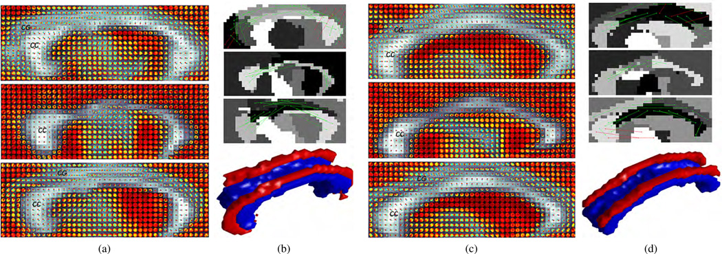
In panels (a) and (c) from top to bottom: Three slices selected from the 3D ROIs of two different subjects, showing the ODFs superimposed on the GFA images. In panels (b) and (d) from top to bottom: Pairwise constraints (must-links in green and cannot-links in red) superimposed on the result of uSRMC, and segmentation of the 3D ODF image using wsSRMC, where the CC are CG are shown in blue and red, respectively.
IV. Conclusion
We have presented a clustering method that uses sparse representations to segment HARDI data described by ODFs into multiple clusters. This framework exploits the Riemannian properties of the space of ODFs to reformulate the problem of computing sparse representations for ODFs. The sparse representations are used for constructing a similarity matrix to which we apply spectral clustering for multi-label segmentation of a given ODF image. To resolve cases in which regions with similar (resp. distinct) diffusion properties belong to different (resp. same) fiber tracts, we modify the similarity matrix to include information about spatial relationships, as well as user-specified pairwise constraints. We have evaluated our method on synthetic, phantom, and real data, and demonstrated the benefits of using supervision, a desirable feature for clinicians to incorporate their expertise in neuroanatomy into segmentation.
Our primary goal for clinical research is to improve the quality of WM atlases by restricting tractography to be within the boundaries of the segmented regions. In the interim, from a technical perspective, future work will initially focus on increasing the speed of SRMC without a severe reduction in segmentation accuracy. In particular, we will investigate
the use of the Nyström method [56] or fast normalized cut [57] for spectral clustering to handle cases with very large numbers of ODFs;
the use of iterative shrinkage-thresholding algorithms [58] or augmented Lagrangian methods [59]–[61] to compute sparse representations;
the idea of decreasing the number of ODFs to be clustered by oversegmenting the image (e.g., using k-means) and considering each cluster as a “super-voxel” in which the mean ODF will describe diffusion.
Possible directions for future research also include developing new formulations that penalize the number of labels [62], and/or identify clusters with multiple labels [63]. This will result in a segmentation where a region with partial volume effects (e.g., a fiber intersection) is identified with the labels of the fibers forming the intersection. Such information may be beneficial for identifying which WM fiber tracts (and hence how structural connectivity) would be affected by impairment in the complex regions of WM.
Acknowledgment
H. Ertan Çetingül performed this work while at The Johns Hopkins University. Brain image collection for this work was supported by the National Institute of Child Health and Human Development (R01 HD050735), and the National Health and Medical Research Council (NHMRC 486682), Australia. The authors would like to thank Katie L. McMahon and Greig I. de Zubicaray at the Centre for Magnetic Resonance, University of Queensland for agreeing to share the brain image data.
This work was supported in part by The Johns Hopkins University Whiting School of Engineering (start-up funds), the Sloan Research Fellowship, and the National Institutes of Health (R01 EB008432).
Appendix
A Modified Spherical Harmonic Basis
The standard normalized spherical harmonic (SH) of degree l and order m is defined as
| (21) |
where is the associated Legendre polynomial and (θ, ϕ) obeys physics convention (θ ∈ [0, π], ϕ ∈ [0, 2π)) [40]. In [23], a modified real and symmetric SH basis is defined to represent real-valued functions with antipodal symmetry, e.g., the HARDI signal. This new basis of degree L contains R = (L + 1)(L + 2)/2 elements Yr of the form
| (22) |
where r := r(l, m) = (l2 + l + 2)/2 + m for l = 0, 2, 4, …, L, m = −l, …, 0, …, l, and and represent the real and imaginary parts of , respectively. In this work, we consider the SH basis of degree L = 4 ⇒ R = 15.
Footnotes
Color versions of one or more of the figures in this paper are available online at http://ieeexplore.ieee.org.
The Funk-Radon transform of a function f at point u∈𝕊2 is defined as FRT{f}(u)= ∫𝕊2 δ(u⊤ v)f(v)dv, where δ(t) is the Dirac delta function.
In this work, we consider the SH basis of degree 4, and hence R=15.
𝒩(μ, σ2) denotes the normal distribution with mean μ and variance σ2.
For NCut, we construct the matrix A = [aij] such that the entries aij =e−κψ dist2(ψi, ψj), where we pick κψ ∈[10, 100] that yields the best performance. For LLMC, we employ the framework in [32] and use 10 nearest neighbors of each ODF to find the embedding.
For the configurations with two curved fibers, we used 5.42 must-link and 3.57 cannot-link constraints per configuration on average, whereas for the configurations with one curved and one linear fiber, we used 3.86 must-link and 2.79 cannot-link constraints on average. The maximum number of pairwise constraints that we enforce are 15 for the former and 10 for the latter.
We illustrate the performance of these methods in Figs. 6a–6d when the number of clusters is set to four to better delineate the boundaries of the U-shaped fiber and to still keep its portion clustered with the linear fiber.
Notice that in Fig. 8d, (and in Figs. 9b and 9d as we shall see next), the segmentation given by uSRMC contains more clusters than the number of clusters we anticipated for the ground truth. The reason behind this choice is to better illustrate the pairwise constraints by superimposing them on oversegmented images for which uSRMC failed to produce a good segmentation using the anticipated number of clusters.
Contributor Information
H. Ertan Çetingül, Imaging and Computer Vision Technology Field, Siemens Corporation, Corporate Technology, Princeton, NJ 08540, USA. (hasan.cetingul@siemens.com).
Margaret J. Wright, Queensland Institute of Medical Research and with the School of Psychology, The University of Queensland, Brisbane 4072, Queensland, Australia (margie.wright@qimr.edu.au)
Paul M. Thompson, Laboratory of Neuro Imaging, Department of Neurology, University of California-Los Angeles (UCLA) School of Medicine, Los Angeles, CA 90095, USA (thompson@loni.ucla.edu)
René Vidal, Department of Biomedical Engineering, The Johns Hopkins University, Baltimore, MD 21218, USA (rvidal@jhu.edu).
References
- 1.Callaghan P. Principles of nuclear magnetic resonance microscopy. Oxford University Press; 1991. [Google Scholar]
- 2.Jones D, editor. Diffusion MRI: Theory, methods, and applications. Oxford University Press; 2011. [Google Scholar]
- 3.Basser P, Mattiello J, LeBihan D. Estimation of the effective self-diffusion tensor from the NMR spin echo. Journal of Magnetic Resonance B. 1994;103(3):247–254. doi: 10.1006/jmrb.1994.1037. [DOI] [PubMed] [Google Scholar]
- 4.Descoteaux M, Deriche R. High angular resolution diffusion MRI segmentation using region-based statistical surface evolution. Journal of Mathematical Imaging and Vision. 2009;33(2):239–252. [Google Scholar]
- 5.Zhukov L, Museth K, Breen D, Whitaker R, Barr A. Level set segmentation and modeling of DT-MRI human brain data. Journal of Electronic Imaging. 2003;12(1):125–133. [Google Scholar]
- 6.Wiegell M, Tuch D, Larsson H, Wedeen V. Automatic segmentation of thalamic nuclei from diffusion tensor magnetic resonance imaging. NeuroImage. 2003;19(2):391–401. doi: 10.1016/s1053-8119(03)00044-2. [DOI] [PubMed] [Google Scholar]
- 7.Ziyan U, Tuch D, Westin C-F. Segmentation of thalamic nuclei from DTI using spectral clustering. In: Larsen R, Nielsen M, Sporring J, editors. Medical Image Computing and Computer-Assisted Intervention - MICCAI 2006, ser. Lecture Notes in Computer Science. Vol. 4191. Springer Berlin / Heidelberg: 2006. pp. 807–814. ser. Lecture Notes in Computer Science. [DOI] [PubMed] [Google Scholar]
- 8.Wang Z, Vemuri BC. Tensor field segmentation using region based active contour model. In: Pajdla T, Matas J, editors. Computer Vision - ECCV 2004, ser. Lecture Notes in Computer Science. Vol. 3024. Springer Berlin / Heidelberg: 2004. pp. 304–315. [Google Scholar]
- 9.Jonasson L, Hagmann P, Pollo C, Bresson X, Richero Wilson C, Meuli R, Thiran J. A level set method for segmentation of the thalamus and its nuclei in DT-MRI. Signal Processing. 2007;87(2):309–321. [Google Scholar]
- 10.Jonasson L, Bresson X, Hagmann P, Cuisenaire O, Meuli R, Thiran J. White matter fiber tract segmentation in DT-MRI using geometric flows. Medical Image Analysis. 2005 Oct;9(3):223–236. doi: 10.1016/j.media.2004.07.004. [DOI] [PubMed] [Google Scholar]
- 11.Wang Z, Vemuri B. DTI segmentation using an information theoretic tensor dissimilarity measure. IEEE Transactions on Medical Imaging. 2005 Oct;24(10):1267–1277. doi: 10.1109/TMI.2005.854516. [DOI] [PubMed] [Google Scholar]
- 12.Lenglet C, Rousson M, Deriche R. DTI segmentation by statistical surface evolution. IEEE Transactions on Medical Imaging. 2006;25(6):685–700. doi: 10.1109/tmi.2006.873299. [DOI] [PubMed] [Google Scholar]
- 13.Goh A, Vidal R. Segmenting fiber bundles in diffusion tensor images. In: Forsyth D, Torr P, Zisserman A, editors. Computer Vision - ECCV 2008, ser. Lecture Notes in Computer Science. Vol. 5304. Springer Berlin / Heidelberg: 2008. pp. 238–250. [Google Scholar]
- 14.Vemuri BC, Liu M, Amari S-I, Nielsen F. Total Bregman divergence and its applications to DTI analysis. IEEE Transactions on Medical Imaging. 2011;30(2):475–483. doi: 10.1109/TMI.2010.2086464. [DOI] [PMC free article] [PubMed] [Google Scholar]
- 15.Xie Y, Chen T, Ho J, Vemuri BC. Multi-class DTI segmentation: A convex approach. MICCAI 2012 Workshop on Computational Diffusion MRI. 2012:115–123. [PMC free article] [PubMed] [Google Scholar]
- 16.Ramirez-Manzanares A, Rivera M. Basis tensor decomposition for restoring intra-voxel structure and stochastic walks for inferring brain connectivity in DT-MRI. International Journal of Computer Vision. 2006;69(1):77–92. [Google Scholar]
- 17.Jian B, Vemuri B. A unified computational framework for deconvolution to reconstruct multiple fibers from diffusion weighted MRI. IEEE Transactions on Medical Imaging. 2007 Nov;26(11):1464–1471. doi: 10.1109/TMI.2007.907552. [DOI] [PMC free article] [PubMed] [Google Scholar]
- 18.Barmpoutis A, Hwang MS, Howland D, Forder JR, Vemuri BC. Regularized positive-definite fourth order tensor field estimation from DW-MRI. NeuroImage. 2009;45(1 Suppl.):S153–S162. doi: 10.1016/j.neuroimage.2008.10.056. [DOI] [PMC free article] [PubMed] [Google Scholar]
- 19.Leow AD, Zhu S, Zhan L, McMahon K, de Zubicaray GI, Meredith M, Wright MJ, Toga AW, Thompson PM. The tensor distribution function. Magnetic Resonance in Medicine. 2009;61(1):205–214. doi: 10.1002/mrm.21852. [DOI] [PMC free article] [PubMed] [Google Scholar]
- 20.Wedeen V, Hagmann P, Tseng W, Reese T, Weisskoff R. Mapping complex tissue architecture with diffusion spectrum magnetic resonance imaging. Magnetic Resonance in Medicine. 2005;54(6):1377–1386. doi: 10.1002/mrm.20642. [DOI] [PubMed] [Google Scholar]
- 21.Tuch D. Q-ball imaging. Magnetic Resonance in Medicine. 2004;52(6):1358–1372. doi: 10.1002/mrm.20279. [DOI] [PubMed] [Google Scholar]
- 22.Tournier J-D, Calamante F, Connelly A. Robust determination of the fibre orientation distribution in diffusion MRI: Non-negativity constrained super-resolved spherical deconvolution. NeuroImage. 2007;35(4):1459–1472. doi: 10.1016/j.neuroimage.2007.02.016. [DOI] [PubMed] [Google Scholar]
- 23.Descoteaux M, Angelino E, Fitzgibbons S, Deriche R. Regularized, fast and robust analytical Q-ball imaging. Magnetic Resonance in Medicine. 2007;58(3):497–510. doi: 10.1002/mrm.21277. [DOI] [PubMed] [Google Scholar]
- 24.Lenglet C, Campbell J, Descoteaux M, Haro G, Savadjiev P, Wassermann D, Anwander A, Deriche R, Pike G, Sapiro G, Siddiqi K, Thompson P. Mathematical methods for diffusion MRI processing. NeuroImage. 2009;45:S111–S122. doi: 10.1016/j.neuroimage.2008.10.054. [DOI] [PMC free article] [PubMed] [Google Scholar]
- 25.Tristan-Vega A, Westin C-F, Aja-Fernandez S. Estimation of fiber orientation probability density functions in high angular resolution diffusion imaging. NeuroImage. 2009;47(2):638–650. doi: 10.1016/j.neuroimage.2009.04.049. [DOI] [PubMed] [Google Scholar]
- 26.Aganj I, Lenglet C, Sapiro G, Yacoub E, Ugurbil K, Harel N. Reconstruction of the orientation distribution function in single- and multiple-shell q-ball imaging within constant solid angle. Magnetic Resonance in Medicine. 2010;64(2):554–566. doi: 10.1002/mrm.22365. [DOI] [PMC free article] [PubMed] [Google Scholar]
- 27.Hagmann P, Jonasson L, Deffieux T, Meuli R, Thiran J-P, Wedeen V. Fibertract segmentation in position orientation space from high angular resolution diffusion MRI. NeuroImage. 2006;32(2):665–675. doi: 10.1016/j.neuroimage.2006.02.043. [DOI] [PubMed] [Google Scholar]
- 28.Jonasson L, Bresson X, Thiran J-P, Wedeen V, Hagmann P. Representing diffusion MRI in 5-D simplifies regularization and segmentation of white matter tracts. IEEE Transactions on Medical Imaging. 2007;26(11):1547–1554. doi: 10.1109/TMI.2007.899168. [DOI] [PubMed] [Google Scholar]
- 29.McGraw T, Vemuri B, Yezierski R, Mareci T. Segmentation of high angular resolution diffusion MRI modeled as a field of von Mises-Fisher mixtures. In: Leonardis A, Bischof H, Pinz A, editors. Computer Vision - ECCV 2006, ser. Lecture Notes in Computer Science. Vol. 3953. Springer Berlin / Heidelberg: 2006. pp. 463–475. [Google Scholar]
- 30.Wassermann D, Descoteaux M, Deriche R. Diffusion maps clustering for magnetic resonance Q-ball imaging segmentation. International Journal of Biomedical Imaging. 2008 doi: 10.1155/2008/526906. [DOI] [PMC free article] [PubMed] [Google Scholar]
- 31.Nazem-Zadeh M-R, Davoodi-Bojd E, Soltanian-Zadeh H. Atlas-based fiber bundle segmentation using principal diffusion directions and spherical harmonic coefficients. NeuroImage. 2011;54(1) Suppl.:S146–S164. doi: 10.1016/j.neuroimage.2010.09.035. [DOI] [PubMed] [Google Scholar]
- 32.Goh A, Vidal R. Clustering and dimensionality reduction on Riemannian manifolds; IEEE Conference on Computer Vision and Pattern Recognition; 2008. pp. 1–7. [Google Scholar]
- 33.Goh A. Unsupervised Riemannian clustering of probability density functions. In: Daelemans W, Goethals B, Morik K, editors. Machine Learning and Knowledge Discovery in Databases, ser. Lecture Notes in Computer Science. Vol. 5211. Springer Berlin / Heidelberg: 2008. pp. 377–392. [Google Scholar]
- 34.Elhamifar E, Vidal R. Sparse subspace clustering; IEEE Conference on Computer Vision and Pattern Recognition; 2009. pp. 2790–2797. [Google Scholar]
- 35.Zhang S, Huang J, Wang W, Huang X, Metaxas D. Discriminative sparse representations for cervigram image segmentation; IEEE International Symposium on Biomedical Imaging; 2010. pp. 133–136. [Google Scholar]
- 36.Yu Y, Huang J, Zhang S, Restif C, Huang X, Metaxas D. Group sparsity based classification for cervigram segmentation; IEEE International Symposium on Biomedical Imaging; 2011. [Google Scholar]
- 37.Goh A, Lenglet C, Thompson P, Vidal R. A nonparametric Riemannian framework for processing high angular resolution diffusion images and its applications to ODF-based morphometry. NeuroImage. 2011;56(3):1181–1201. doi: 10.1016/j.neuroimage.2011.01.053. [DOI] [PMC free article] [PubMed] [Google Scholar]
- 38.Goh A. Estimating orientation distribution functions with probability density constraints and spatial regularity. In: Yang G-Z, Hawkes D, Rueckert D, Noble A, Taylor C, editors. Medical Image Computing and Computer-Assisted Intervention - MICCAI 2009, ser. Lecture Notes in Computer Science. Vol. 5761. Springer Berlin / Heidelberg: 2009. pp. 877–885. [DOI] [PubMed] [Google Scholar]
- 39.Çetingül HE, Vidal R. Sparse Riemannian manifold clustering for HARDI segmentation; IEEE International Symposium on Biomedical Imaging; 2011. pp. 1750–1753. [Google Scholar]
- 40.Chirikjian G, Kyatkin A. Engineering Applications of Noncommutative Harmonic Analysis: With Emphasis on Rotation and Motion Groups. CRC Press; 2000. [Google Scholar]
- 41.Rao C. Information and accuracy attainable in the estimation of statistical parameters. Bulletin of the Calcutta Mathematical Society. 1945;37:81–89. [Google Scholar]
- 42.Cencov NN. Statistical decision rules and optimal inference. Vol. 53 Translations of Mathematical Monographs, AMS; 1982. [Google Scholar]
- 43.Srivastava A, Jermyn I, Joshi S. Riemannian analysis of probability density functions with applications in vision; IEEE Conference on Computer Vision and Pattern Recognition; 2007. pp. 1–8. [DOI] [PMC free article] [PubMed] [Google Scholar]
- 44.Bhattacharyya A. On a measure of divergence between two statistical populations defined by their probability distributions. Bulletin of the Calcutta Mathematical Society. 1943;35:99–110. [Google Scholar]
- 45.Vidal R. Subspace clustering. IEEE Signal Processing Magazine. 2011 Mar;28(3):52–68. [Google Scholar]
- 46.von Luxburg U. A tutorial on spectral clustering. Statistics and Computing. 2007;17 [Google Scholar]
- 47.Becker S, Bobin J, Candès E. NESTA: A fast and accurate first-order method for sparse recovery. California Institute of Technology, Tech. Rep. 2009 Apr [Google Scholar]
- 48.Lu Z, Carreira-Perpiñán M. Constrained spectral clustering through affinity propagation; IEEE Conference on Computer Vision and Pattern Recognition; 2008. pp. 1–8. [Google Scholar]
- 49.Shi J, Malik J. Normalized cuts and image segmentation. IEEE Transactions on Pattern Analysis and Machine Intelligence. 2000;22(8):888–905. [Google Scholar]
- 50.Dice L. Measures of the amount of ecologic association between species. Ecology. 1945;26(3):297–302. [Google Scholar]
- 51.Cheng J, Ghosh A, Jiang T, Deriche R. A Riemannian framework for orientation distribution function computing. In: Yang G-Z, Hawkes D, Rueckert D, Noble A, Taylor C, editors. Medical Image Computing and Computer-Assisted Intervention - MICCAI 2009, ser. Lecture Notes in Computer Science. Vol. 5761. Springer Berlin / Heidelberg: 2009. pp. 911–918. [DOI] [PubMed] [Google Scholar]
- 52.Fillard P, Descoteaux M, Goh A, Gouttard S, Jeurissen B, Malcolm J, Ramirez-Manzanares A, Reisert M, Sakaike K, Tensaouti F, Yo T, Mangin J-F, Poupon C. Quantitative evaluation of 10 tractography algorithms on a realistic diffusion MR phantom. NeuroImage. 2011;56:220–234. doi: 10.1016/j.neuroimage.2011.01.032. [DOI] [PubMed] [Google Scholar]
- 53.Poupon C, Rieul B, Kezele I, Perrin M, Poupon F, Mangin J-F. New diffusion phantoms dedicated to the study and validation of high-angular-resolution diffusion imaging (HARDI) models. Magnetic Resonance in Medicine. 2008;60(6):1276–1283. doi: 10.1002/mrm.21789. [DOI] [PubMed] [Google Scholar]
- 54.Chiang M-C, Barysheva M, Lee A, Madsen S, Klunder A, Toga A, McMahon K, de Zubicaray G, Meredith M, Wright M, Srivastava A, Balov N, Thompson P. Brain fiber architecture, genetics, and intelligence: A high angular resolution diffusion imaging (HARDI) study. In: Metaxas D, Axel L, Fichtinger G, Székely G, editors. Medical Image Computing and Computer-Assisted Intervention - MICCAI 2008, ser. Lecture Notes in Computer Science. Vol. 5241. Springer Berlin / Heidelberg: 2008. pp. 1060–1067. [DOI] [PMC free article] [PubMed] [Google Scholar]
- 55.Chiang M, Dutton R, Hayashi K, Lopez O, Aizenstein H, Toga A, Becker J, Thompson P. 3D pattern of brain atrophy in HIV/AIDS visualized using tensor-based morphometry. NeuroImage. 2007;34(1):44–60. doi: 10.1016/j.neuroimage.2006.08.030. [DOI] [PMC free article] [PubMed] [Google Scholar]
- 56.Folwkes C, Belongie S, Chung F, Malik J. Spectral grouping using the Nyström method. IEEE Transactions on Pattern Analysis and Machine Intelligence. 2004;26(2):214–225. doi: 10.1109/TPAMI.2004.1262185. [DOI] [PubMed] [Google Scholar]
- 57.Dhillon I, Guan Y, Kulis B. Weighted graph cuts without eigenvectors: A multilevel approach. IEEE Transactions on Pattern Analysis and Machine Intelligence. 2007;29(11):1944–1957. doi: 10.1109/TPAMI.2007.1115. [DOI] [PubMed] [Google Scholar]
- 58.Beck A, Teboulle M. A fast iterative shrinkage-thresholding algorithm for linear inverse problems. SIAM Journal on Imaging Sciences. 2009;2(1):183–202. [Google Scholar]
- 59.Aybat N, Iyengar G. A first-order augmented Lagrangian method for compressed sensing. arXiv:1005.5582v2. 2011 [Google Scholar]
- 60.Boyd S, Parikh N, Chu E, Peleato B, Eckstein J. Distributed optimization and statistical learning via the alternating direction method of multipliers. Foundations and Trends in Machine Learning. 2010;3(1):1–122. [Google Scholar]
- 61.Elhamifar E, Vidal R. Sparse subspace clustering: Algorithm, theory, and applications. 2012 doi: 10.1109/TPAMI.2013.57. http://arxiv.org/abs/1203.1005. [DOI] [PubMed] [Google Scholar]
- 62.Delong A, Osokin A, Isack H, Boykov Y. Fast approximate energy minimization with label costs; IEEE Conference on Computer Vision and Pattern Recognition; 2010. pp. 2173–2180. [Google Scholar]
- 63.Russell C, Fayad J, Agapito L. Energy based multiple model fitting for non-rigid structure from motion; IEEE Conference on Computer Vision and Pattern Recognition; 2011. pp. 3009–3016. [Google Scholar]