Efficient modeling of vector hysteresis using a novel Hopfield neural network implementation of Stoner–Wohlfarth-like operators

Abstract

Incorporation of hysteresis models in electromagnetic analysis approaches is indispensable to accurate field computation in complex magnetic media. Throughout those computations, vector nature and computational efficiency of such models become especially crucial when sophisticated geometries requiring massive sub-region discretization are involved. Recently, an efficient vector Preisach-type hysteresis model constructed from only two scalar models having orthogonally coupled elementary operators has been proposed. This paper presents a novel Hopfield neural network approach for the implementation of Stoner–Wohlfarth-like operators that could lead to a significant enhancement in the computational efficiency of the aforementioned model. Advantages of this approach stem from the non-rectangular nature of these operators that substantially minimizes the number of operators needed to achieve an accurate vector hysteresis model. Details of the proposed approach, its identification and experimental testing are presented in the paper.

Introduction

Incorporation of hysteresis models in electromagnetic analysis approaches is indispensable to accurate field computation in complex magnetic media (refer, for instance, to [1–3]). Examples of applications requiring such sophisticated field computation approaches include harmonic and loss estimation of power devices, magnetic recording processes and design of magnetostrictive actuators [4,5]. Throughout those applications, vector nature and computational efficiency of such models become especially crucial when sophisticated geometries requiring massive sub-region discretization are involved.

Recently, an efficient vector Preisach-type hysteresis model constructed from only two scalar models having orthogonally coupled elementary operators has been proposed [6,7]. This model was implemented via a linear neural network (LNN) whose inputs were four-node discrete Hopfield neural network (DHNN) blocks having step activation functions. Given this DHNN–LNN configuration, it was possible to carry out the identification process using well established widely available NN algorithms.

This paper presents a novel Hopfield neural network approach for the implementation of Stoner–Wohlfarth-like operators that could lead to a significant enhancement in the computational efficiency of the aforementioned model [8]. Advantages of this approach stem from the non-rectangular nature of these operators that substantially minimizes the number of operators needed to achieve an accurate vector hysteresis model. Details of the proposed approach, its identification and experimental testing are presented in the following sections.

Proposed methodology

It has been previously shown that an elementary hysteresis operator may be realized using a two-node discrete Hopfield neural network (HNN) having step activation functions and positive feedback weights [9]. In a discrete HNN, node inputs and outputs (or states) are discrete with values of either −1 or 1. Each node applies a step activation function to the sum of its external input and the weighted outputs of the other nodes. The activation function, fd(x), is the signum function where:

$$\mathit{fd}(x)=\left\{\begin{array}{ccc}+1\hfill & \text{if}\hfill & x>0\hfill \\ -1\hfill & \text{if}\hfill & x<0\hfill \\ \text{unchanged}\hfill & \text{if}\hfill & x=0\hfill \end{array}\right)$$ (1)

In a continuous HNN, on the other hand, node inputs and outputs are continuous with values in the interval [−1, 1]. Node activation functions are continuous and differentiable everywhere, symmetric about the origin, and asymptotically approach their saturation values of −1 and 1. An example of such an activation function fc(x) may be given by:

$$\mathit{fc}(x)=\tanh (\mathit{ax})$$ (2)

where a is some positive constant.

Each node constantly examines its net input and updates its output accordingly. As a result of external inputs, node output values may change until the network converges to the minimum of its energy function [10].

Consider a general two-node HNN with positive feedback weights as shown in Fig. 1a. Whether the HNN activation function is continuous or discrete, the energy function may be expressed in the form:

$$E=-[I(U_A+U_B)+{\mathit{kU}}_A{U}_B]$$ (3)

where I is the HNN input, U_A is the output of node A, U_B is the output of node B and k is the positive feedback between nodes A and B.

Fig. 1.

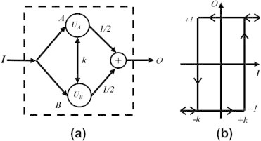
Implementation of an elementary rectangular hysteresis operator using a two-node HNN having discrete activation function: (a) the HNN configuration and (b) the input–output hysteresis relation.

Following the gradient descent rule for the discrete case, the output of say node A is changed as:

$$U_A(t+1)=\mathit{fd}(\mathit{net}(t))\text{,}\text{where}\mathit{net}(t)={\mathit{kU}}_B(t)+I$$ (4)

Using the same gradient descent rule for the continuous case, the output is changed gradually as:

$$\frac{\delta U_A}{\delta t}=\eta \mathit{fc}(\mathit{net}(t))\text{,}\text{where}\mathit{net}(t)={\mathit{kU}}_B(t)+I$$ (5)

In (5), η is a small positive learning rate that controls the convergence speed.

It should be stressed here that using continuous activation function will result in a single-valued input–output relation. On the other hand, a discrete activation function will result in the primitive rectangular hysteresis operator shown in Fig. 1b. The non-smooth nature of this rectangular building block suggests that a realistic simulation of a typical magnetic material hysteretic property will require a superposition of a relatively large number of those blocks (refer, for instance, to Mayergoyz [11]).

In order to obtain a smoother operator, a new hybrid activation function is introduced in this paper. More specifically, the proposed activation function may be expressed in the form:

$$f(x)=\mathit{cfc}(x)+\mathit{dfd}(x)$$ (6)

where c and d are two positive constants such that c + d = 1. The function f(x) is piecewise continuous with a single discontinuity at the origin. The choice of the two constants, c and d, controls the slopes with which the function asymptotically approaches the saturation values of −1 and 1. In this case, the new hybrid activation rule for, say, node A becomes:

$$U_A(t+1)=\mathit{cfc}(\mathit{net}(t))+\mathit{dfd}(\mathit{net}(t))$$ (7)

where net(t) is defined as before. Fig. 2 depicts the smooth hysteresis operator resulting from the novel two-node hybrid HNN. The figure illustrates how the hybrid activation function results in smooth Stoner–Wohlfarth-like hysteresis operators with controllable loop width and squareness. In particular, within this implementation the loop width is equivalent to the product 2kd while the squareness is controlled by the ratio c/d.

Fig. 2.

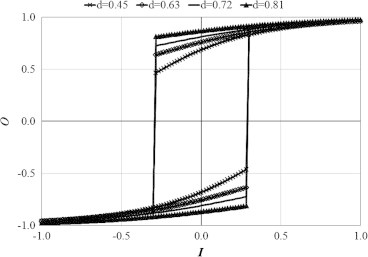
Proposed novel hybrid HNN implementation of smooth Stoner–Wohlfarth-like hysteresis operators with controllable loop width and squareness (k = 0.48/d for all curves, thus maintain constant loop width).

Extrapolating the proposed implementation to the vector hysteresis modeling approach presented by Adly and Abd-El-Hafiz [6], consider the four-node HNN network shown in Fig. 3. In this Fig, kc denotes a coupling factor between nodes corresponding to different vectorial directions. Indeed, this network is capable of realizing a couple of smooth Stoner–Wohlfarth-like hysteresis whose inputs Ix, Iy and outputs Ox, Oy correspond to the x- and y-directions. The state of this network converges to the minimum of the following energy function:

$$E=-\left\{\begin{array}{c}\hfill \mathit{Ix}(U_{\mathit{Ax}}+U_{\mathit{Bx}})+{\mathit{kU}}_{\mathit{Ax}}{U}_{\mathit{Bx}}+\mathit{Iy}(U_{\mathit{Ay}}+U_{\mathit{By}})+{\mathit{kU}}_{\mathit{Ay}}{U}_{\mathit{By}}+\hfill \\ \hfill \frac{\mathit{kc}}{2}(U_{\mathit{Ax}}-U_{\mathit{Bx}})(U_{\mathit{Ay}}+U_{\mathit{By}})+\frac{\mathit{kc}}{2}(U_{\mathit{Ay}}-U_{\mathit{By}})(U_{\mathit{Ax}}+U_{\mathit{Bx}})\hfill \end{array}\right\}$$ (8)

where node outputs are updated in accordance with the following expressions:

$$U_{\mathit{Ax}}(t+1)=\mathit{cfc}({\mathit{net}}_{\mathit{Ax}}(t))+\mathit{dfd}({\mathit{net}}_{\mathit{Ax}}(t))\text{,}{\mathit{net}}_{\mathit{Ax}}(t)=\mathit{Ix}+{\mathit{kU}}_{\mathit{Bx}}(t)+\mathit{kc}(U_{\mathit{Ay}}(t)+U_{\mathit{By}}(t))$$ (9)

$$U_{\mathit{Bx}}(t+1)=\mathit{cfc}({\mathit{net}}_{\mathit{Bx}}(t))+\mathit{dfd}({\mathit{net}}_{\mathit{Bx}}(t))\text{,}{\mathit{net}}_{\mathit{Bx}}(t)=\mathit{Ix}+{\mathit{kU}}_{\mathit{Ax}}(t)-\mathit{kc}(U_{\mathit{Ay}}(t)+U_{\mathit{By}}(t))$$ (10)

$$U_{\mathit{Ay}}(t+1)=\mathit{cfc}({\mathit{net}}_{\mathit{Ay}}(t))+\mathit{dfd}({\mathit{net}}_{\mathit{Ay}}(t))\text{,}{\mathit{net}}_{\mathit{Ay}}(t)=\mathit{Iy}+{\mathit{kU}}_{\mathit{By}}(t)+\mathit{kc}(U_{\mathit{Ax}}(t)+U_{\mathit{Bx}}(t))$$ (11)

$$U_{\mathit{By}}(t+1)=\mathit{cfc}({\mathit{net}}_{\mathit{By}}(t))+\mathit{dfd}({\mathit{net}}_{\mathit{By}}(t))\text{,}{\mathit{net}}_{\mathit{By}}(t)=\mathit{Iy}+{\mathit{kU}}_{\mathit{Ay}}(t)-\mathit{kc}(U_{\mathit{Ax}}(t)+U_{\mathit{Bx}}(t))$$ (12)

Fig. 3.

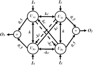
A four-node HNN having hybrid activation function capable of realizing two orthogonally coupled smooth Stoner–Wohlfarth-like hysteresis operators.

There is no doubt that if the input is restricted to vary along a single direction, output behavior will be as shown in Fig. 2. The far-reaching capabilities of the proposed four-node hybrid HNN, however, may be demonstrated when vector input–output variations are considered. For instance, consider output components Ox, Oy resulting from a rotating unit input value and corresponding to different k, c and d values as shown in Fig. 4. This figure clearly demonstrates two facts. First, it demonstrates that the qualitatively expected rotational behavior may be quantitatively tuned. Second, it stresses the smoothly varying nature of the proposed hybrid HNN outputs in comparison to previously reported results based upon primitive rectangular hysteresis building blocks (refer Adly and Abd-El-Hafiz [6]). Those two facts are further highlighted by the results shown in Fig. 5 which demonstrate how mutually correlation between orthogonal inputs and outputs of the proposed HNN may be tuned. In this figure, initial Oy components and remnant Ox components, which are initially achieved by increasing Ix to unity then back to zero, are plotted versus an increasing Iy input for different coupling and d values.

Fig. 4.

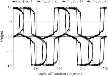
Output x- and y-components of the proposed HNN resulting from a rotating unit value input (k = 0.48/d and kc = 0.3).

Fig. 5.

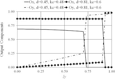
Correlation between mutually orthogonal input–output components for the proposed HNN (k = 0.48/d).

Building up on the reasoning previously presented by Adly and Abd-El-Hafiz [6] and making use of the significant scalar and vector results shown in Figs. 2, 4, and 5 corresponding to the proposed HNN block, a computationally efficient Preisach-type vector hysteresis model comprised of a reduced number of blocks may be constructed. In particular, this vector hysteresis model is constructed from an ensemble of vector operators, each being realized by the proposed hybrid activation function four-node HNN. Since the ensemble of blocks should correspond to loops having different widths and/or center shifts, different feedback values as well as input offsets should be imposed. It should be stated here that while a vector-type behavior of a single block is not perfectly isotropic, a superposition of blocks (having different coupling and offset values) would significantly lead to isotropicity. Moreover, computational efficiency is enhanced as a result of the incorporation of smooth non-primitive Stoner–Wohlfarth-like operators that only need to cover the hysteretic loop zone. Since this zone is usually restricted within the coercive field values (i.e., covers no more than 50% of a typical loop domain), the proposed implementation could, reduce the number of block ensembles needed to construct a vector hysteresis model to only (50%)² = 25% of those needed in a typical implementation.

Referring to the typical configuration of a Preisach-type model [11] as well as the proposed hybrid activation function four-node HNN, a vector magnetic hysteresis model may then be constructed as depicted in Fig. 6. The configuration under consideration is, basically, a modular combination of the proposed HNN blocks via a linear neural network (LNN) structure. In Fig. 6, Hx, Hy, Mx, My, OS_i and μ_i represent the applied field x-component, the applied field y-component, the computed x-component magnetization, the computed y-component magnetization, the applied field imposed offset corresponding to the ith HNN block and a density value corresponding to the ith HNN block, respectively. As previously stated, the advantage of the proposed methodology is clearly highlighted in restricting offset values OS and positive feedback factors k to generate an ensemble of Stoner–Wohlfarth-like smooth operators within the hysteretic loop zone only. More specifically, for a particular operator whose switching up and down thresholds are given by α_i and β_i, respectively, its corresponding ith HNN imposed OS_i and k_i may be given by:

$${\mathit{OS}}_i=-\left(\frac{{\alpha }_i+{\beta }_i}{2}\right)\text{and}{k}_i=\left(\frac{{\alpha }_i-{\beta }_i}{2}\right)\text{,}\text{where}{\alpha }_i>{\beta }_i$$ (13)

Fig. 6.

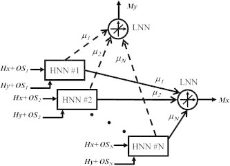
Implementation of the vector Preisach-type model of magnetic hysteresis using a modular combination of the proposed HNN blocks and LNN structure.

It should be noted that while the ratio between d and c = (1 − d) could affect the shape of a hysteresis operator, this ratio has no effect on its switching thresholds α and β but rather on the squareness of the loop. Moreover, varying the coupling factor kc would mainly affect the vector performance of an HNN block.

Considering a finite number N of the proposed HNN blocks – as shown in Fig. 6 – identification of the model unknowns is thus reduced to appropriate selection of d (which implicitly defines c), appropriate selection of coupling factors kc and determination of the unknown HNN block density values μ_i.

With the assumption that d (and consequently c) and kc are pre-set, the modular HNN network shown in Fig. 6 is expected to evolve – as a result of any applied input – by changing output states of the HNN blocks such that the following minimum quadratic energy function is achieved:

$$E=-{\displaystyle \sum _{i=1}^N}\left\{\begin{array}{c}(\mathit{Hx}-{\mathit{OS}}_i)(U_{\mathit{Axi}}+U_{\mathit{Bxi}})+(\mathit{Hy}-{\mathit{OS}}_i)(U_{\mathit{Ayi}}+U_{\mathit{Byi}})\hfill \\ +k_i{U}_{\mathit{Axi}}{U}_{\mathit{Bxi}}+k_i{U}_{\mathit{Ayi}}{U}_{\mathit{Byi}}\hfill \\ +\frac{\mathit{kc}}{2}(U_{\mathit{Axi}}-U_{\mathit{Bxi}})(U_{\mathit{Ayi}}+U_{\mathit{Byi}})+\frac{\mathit{kc}}{2}(U_{\mathit{Ayi}}-U_{\mathit{Byi}})U_{\mathit{Axi}}+U_{\mathit{Bxi}})\hfill \end{array}\right\}$$ (14)

where OS_i and k_i are as given in (13).

In this case, the network (i.e., model) outputs may be expressed as:

$$\mathit{Mx}={\displaystyle \sum _{i=1}^N}{\mu }_i\left(\frac{U_{\mathit{Axi}}+U_{\mathit{Bxi}}}{2}\right)\text{,}\mathit{My}={\displaystyle \sum _{i=1}^N}{\mu }_i\left(\frac{U_{\mathit{Ayi}}+U_{\mathit{Byi}}}{2}\right)$$ (15)

It turns out that as a result of the pre-described HNN–LNN configuration, it is indeed possible to carry out the vector Preisach-type model identification process using an automated training algorithm. As a result of this algorithm, any available set of scalar and vector data may be utilized in the identification process.

The identification process is carried out by first making some d and kc assumptions launching the automated training process using available scalar training data. Thus, appropriate μ_i values are determined during this training phase using the available scalar data provided to the network and the least-mean-square (LMS) algorithm implicitly adopted in the LNN neuron whose output corresponds to Mx. Since d is closely related to the hysteresis loop squareness, the training process is repeated to identify the optimum value of this parameter that would lead to the minimum matching error with the available scalar data. Once the scalar data training process is completed, available vector training data may then be utilized to determine the optimum kc value.

Simulations and experimental results

In order to evaluate the validity and efficiency of the proposed approach, simulations and experimental testing have been carried out. Measurements acquired for a floppy disk sample, using a vibrating sample magnetometer equipped with rotational capability, have been utilized for this purpose. Although the H and M limits of the simulated magnetic hysteresis curve were normalized (i.e., restricted to ±1), it was only sufficient to utilize proposed Stoner–Wohlfarth-like operators whose switching values were uniformly distributed subject to the inequalities $-0.45⩽\alpha \text{,}\beta ⩽+0.45\text{,}\text{and}\alpha ⩾\beta$. Consequently, only about 400 HNN blocks were utilized as opposed to 1830 DHNN blocks in the approach presented by Adly and Abd-El-Hafiz [6]. Moreover, since μ_i values corresponding to operators whose switching values are symmetric with respect to the α = −β line should be the same as explained by Mayergoyz [11], unknown block density values were reduced to about 200 (as opposed to 1000 for the approach previously reported by Adly and Abd-El-Hafiz [6]).

During the identification (i.e., training) phase a set of first-order reversal curves – comprised of 960 Hx–Mx pairs – representing the scalar training data was used through the LNN algorithm to determine the unknown μ_i. Mean square error was calculated over the whole training cycle and the training cycle was repeated until the mean square error reached an acceptable value (which was in the order of 10⁻² in this case). This whole process was repeated for different pre-set d (and consequently c) and kc values. Sample results for this training phase corresponding to d = 0.1 and d = 0.5 (i.e., c = 0.9 and c = 0.5) are shown in Figs. 7 and 8, respectively. In each of these two figures, results are given for kc values of 0.6, 0.8 and 1.0. Those results clearly demonstrate that scalar data is more sensitive to d rather than kc values. The same results also demonstrate that the best match with scalar training data was achieved by considering the computed μ_i values corresponding to d = 0.5 (i.e., Fig. 8). It should be pointed out here that the number of iterations required to train both the LNN under consideration and that reported by Adly and Abd-El-Hafiz [6] are proportional to the number of data points. Since both neural networks which assemble the DHNN blocks are linear, the reduction in the computation time gained by adopting the proposed approach is proportional to the reduction in the number of blocks.

Fig. 7.

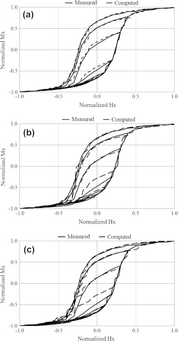
Comparison between the measured and computed first-order-reversal curves at the end of the scalar training (identification) process corresponding to d = 0.1 for; (a) kc = 0.6, (b) kc = 0.8, and (c) kc = 1.0.

Fig. 8.

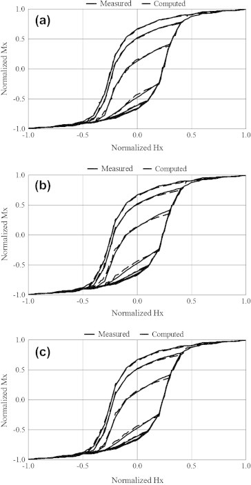
Comparison between the measured and computed first-order-reversal curves at the end of the scalar training (identification) process corresponding to d = 0.5 for; (a) kc = 0.6, (b) kc = 0.8, and (c) kc = 1.0.

To determine the most appropriate kc value, vector measurements were utilized in the second identification phase. Namely, rotational experimental measurements were utilized. Measurements were acquired by first reducing the field along the x-axis to a negative value large enough to drive the magnetization to almost negative saturation, then increased to some value Hr. The field was then fixed in magnitude and rotated with respect to the sample, yielding two magnetization components; a fixed one along the x-axis, and a rotating component which lags Hr. It should be pointed out here that the fixed component vanishes as the rotating field magnitude approaches the saturation field value [11]. This sequence was repeated for different Hr values and the rotational magnetization components parallel and orthogonal to Hr (denoted by $M\_\mathit{parallel}\text{and}M\_\mathit{orthogonal}$) were recorded. Measured and computed results corresponding to the d and kc values of Fig. 8 are shown in Fig. 9. Results shown in this figure clearly demonstrate very good qualitative and quantitative match between measured and computed results for kc = 1.0. By the end of this identification phase all model unknowns (i.e., μ_i, d, c = 1 − d and kc) are found.

Fig. 9.

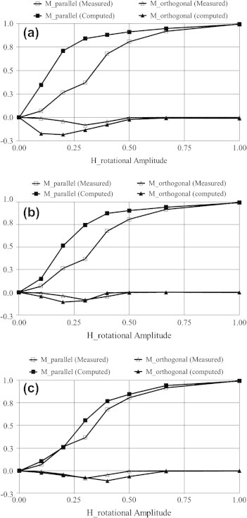
Comparison between the measured and computed rotational data corresponding to d = 0.5 for; (a) kc = 0.6, (b) kc = 0.8, and (c) kc = 1.0.

Further testing of the model accuracy was carried out by comparing its simulation results with other vector magnetization data that was not involved in the identification process. More precisely, a set of vector measurements correlating mutually orthogonal field and magnetization values was utilized. In these measurements, the field was first reduced along the x-axis to a negative value large enough to drive the magnetization to almost negative saturation then increased to some value $\mathit{Hx}\_\mathit{corr}$ and back to zero. This resulted in some residual magnetization component along the x-axis. The field was then increased along the y-axis to a positive value large enough to drive the y-axis magnetization to almost positive saturation while monitoring both Hy and Mx variations. This sequence was repeated for different $\mathit{Hx}\_\mathit{corr}$ values. Measured and computed results corresponding to the pre-identified model unknowns are shown in Fig. 10. Prediction accuracy of the proposed model is clearly demonstrated in this figure.

Fig. 10.

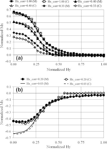
Comparison between the measured and computed orthogonally correlated Hy–Mx data corresponding to the pre-identified model unknowns for; (a) positive residual magnetization and (b) negative residual magnetization.

Discussion and conclusions

It has been shown that the proposed HNN approach for the implementation of Stoner–Wohlfarth-like operators in a Preisach-type vector hysteresis model could lead to a significant enhancement in computational efficiency without compromising accuracy. Moreover, the identification problem of the proposed modular hybrid HNN–LNN implementation may utilize automated well-established neural network algorithms. Figs. 8–10 clearly highlight the implementation ability to match scalar and vector hysteresis data with significant qualitative and quantitative accuracy. Results reported in this paper suggest that further enhancement of the proposed implementation may have wider applications in other coupled physical problems.

References

- 1.Friedman G., Mayergoyz I.D. Computation of magnetic field in media with hysteresis. IEEE Trans Magn. 1989;25:3934–3936. [Google Scholar]
- 2.Adly A.A., Mayergoyz I.D., Gomez R.D., Burke E.R. Computation of magnetic fields in hysteretic media. IEEE Trans Magn. 1993;29:2380–2382. [Google Scholar]
- 3.Saitz J. Newton–Raphson method and fixed-point technique in finite element computation of magnetic field problems in media with hysteresis. IEEE Trans Magn. 1999;35:1398–1401. [Google Scholar]
- 4.Adly A.A. Controlling linearity and permeability of iron core inductors using field orientation techniques. IEEE Trans Magn. 2001;37:2855–2857. [Google Scholar]
- 5.Adly A.A., Davino D., Giustiniani A., Visone C. Experimental tests of a magnetostrictive energy harvesting device and its modeling. J Appl Phys. 2010;107:09A935. [Google Scholar]
- 6.Adly A.A., Abd-El-Hafiz S.K. Efficient implementation of vector Preisach-type models using orthogonally coupled hysteresis operators. IEEE Trans Magn. 2006;42:1518–1525. [Google Scholar]
- 7.Adly A.A., Abd-El-Hafiz S.K. Efficient implementation of anisotropic vector Preisach-type models using coupled step functions. IEEE Trans Magn. 2007;43:2962–2964. [Google Scholar]
- 8.Stoner E.C., Wohlfarth E.P. A mechanism of magnetic hysteresis in heterogeneous alloys. Philos Trans R Soc Lond. 1948;A240:599–642. [Google Scholar]
- 9.Adly A.A., Abd-El-Hafiz S.K. Identification and testing of an efficient Hopfield neural network magnetostriction model. J Magn Magn Mater. 2003;263:301–306. [Google Scholar]
- 10.Mehrotra K., Mohan C.K., Ranka S. The MIT Press; Cambridge, MA: 1997. Elements of artificial neural networks. [Google Scholar]
- 11.Mayergoyz ID. Mathematical models of hysteresis and their applications. New York, NY: Elsevier Science Inc.; 2003.