Utilizing neural networks in magnetic media modeling and field computation: A review

Abstract

Magnetic materials are considered as crucial components for a wide range of products and devices. Usually, complexity of such materials is defined by their permeability classification and coupling extent to non-magnetic properties. Hence, development of models that could accurately simulate the complex nature of these materials becomes crucial to the multi-dimensional field-media interactions and computations. In the past few decades, artificial neural networks (ANNs) have been utilized in many applications to perform miscellaneous tasks such as identification, approximation, optimization, classification and forecasting. The purpose of this review article is to give an account of the utilization of ANNs in modeling as well as field computation involving complex magnetic materials. Mostly used ANN types in magnetics, advantages of this usage, detailed implementation methodologies as well as numerical examples are given in the paper.

Introduction

Magnetic materials are currently regarded as crucial components for a wide range of products and/or devices. In general, the complexity of a magnetic material is defined by its permeability classification as well as its coupling extent to non-magnetic properties (refer, for instance, to [1]). Obviously, development of models that could accurately simulate the complex and, sometimes, coupled nature of these materials becomes crucial to the multi-dimensional field-media interactions and computations. Examples of processes where such models are required include; assessment of energy loss in power devices involving magnetic cores, read/write recording processes, tape and disk erasure approaches, development of magnetostrictive actuators, and energy-harvesting components.

In the past few decades, ANNs have been utilized in many applications to perform miscellaneous tasks such as identification, approximation, optimization, classification and forecasting. Basically, an ANN has a labeled directed graph structure where nodes perform simple computations and each connection conveys a signal from one node to another. Each connection is labeled by a weight indicating the extent to which a signal is amplified or attenuated by the connection. The ANN architecture is defined by the way nodes are organized and connected. Furthermore, neural learning refers to the method of modifying the connection weights and, hence, the mathematical model of learning is another important factor in defining ANNs [2].

The purpose of this review article is to give an account of the utilization of ANNs in modeling as well as field computation involving complex magnetic materials. Mostly used ANN types in magnetics and the advantages of this usage are presented. Detailed implementation methodologies as well as numerical examples are given in the following sections of the paper.

Overview of commonly used artificial neural networks in magnetics

For more than two decades, ANNs have been utilized in various electromagnetic applications ranging from field computation in nonlinear magnetic media to modeling of complex magnetic media. In these applications, different neural architectures and learning paradigms have been used. Fully connected networks and feed-forward networks are among the commonly used architectures. A fully connected architecture is the most general architecture in which every node is connected to every node. On the other hand, feed-forward networks are layered networks in which nodes are partitioned into subsets called layers. There are no intra-layer connections and a connection is allowed from a node in layer i only to nodes in layer i + 1.

As for the learning paradigms, the tasks performed using neural networks can be classified as those requiring supervised or unsupervised learning. In supervised learning, training is used to achieve desired system response through the reduction of error margins in system performance. This is in contrast to unsupervised learning where no training is performed and learning relies on guidance obtained by the system examining different sample data or the environment.

The following subsections present an overview of some ANNs, which have been commonly used in electromagnetic applications. In this overview, both the used neural architecture and learning paradigm are briefly described.

Feed-Forward Neural Networks (FFNN)

FFNN are among the most common neural nets in use. Fig. 1a depicts an example FFNN, which has been utilized in several publications [3–7]. According to this Fig. the 2-layer FFNN consists of an input stage, one hidden layer, and an output layer of neurons successively connected in a feed-forward fashion. Each neuron employs a bipolar sigmoid activation function, f_sig, to the sum of its inputs. This function produces negative and positive responses ranging from −1 to +1 and one of its possible forms can be:

$$f_{\mathit{sig}}(x)=\frac{2}{1+e^{-x}}-1\text{.}$$ (1)

In this network, unknown branch weights link the inputs to various nodes in the hidden layer (W₀₁) as well as link all nodes in hidden and output layers (W₁₂).

Fig. 1.

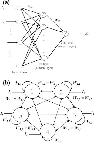
(a) An example 2-layer FFNN, and (b) an example 5-node HNN.

The network is trained to achieve the required input–output response using an error back-propagation training algorithm [8]. The training process starts with a random set of branch weights. The network incrementally adjusts its weights each time it sees an input–output pair. Each pair requires two stages: a feed-forward pass and a back-propagation pass. The weight update rule uses a gradient-descent method to minimize an error function that defines a surface over weight space. Once the various branch weights W₀₁ and W₁₂ are found, it is then possible to use the network, in the testing phase, to generate the output for given set of inputs.

Continuous Hopfield Neural Networks (CHNN)

CHNN are single-layer feedback networks, which operate in continuous time and with continuous node, or neuron, input and output values in the interval [−1, 1]. As shown in Fig. 1b, the network is fully connected with each node i connected to other nodes j through connection weights W_i,j. The output, or state, of node i is called A_i and I_i is its external input. The feedback input to neuron i is equal to the weighted sum of neuron outputs A_j, where j = 1, 2, … , N and N is the number of CHNN nodes. If the matrix W is symmetric with W_ij = W_ji, the total input of neuron i may be expressed as ${\sum }_{j=1}^N{W}_{\mathit{ij}}{A}_j+I_i$.

The node outputs evolve with time so that the Hopfield network converges toward the minimum of any quadratic energy function E formulated as follows [2]:

$$E=-\frac{1}{2}{\displaystyle \sum _{i=1}^N}{\displaystyle \sum _{j=1}^N}{W}_{\mathit{ij}}{A}_i{A}_j-{\displaystyle \sum _{i=1}^N}{I}_i{A}_i+\text{constant.}$$ (2)

The search for the minimum is performed by modifying the state of the network in the general direction of the negative gradient of the energy function. Because the matrix W is symmetric and does not depend on A_i values, then,

$$\frac{\partial E}{\partial A_i}=-{\displaystyle \sum _{j=1}^N}{W}_{\mathit{ij}}{A}_j(t)-I_i\text{.}$$ (3)

Consequently, the state of node i at time t is updated as:

$$\frac{\partial A_i(t)}{\partial t}=\eta \mathit{fc}({\mathit{net}}_i(t))\text{,}{\mathit{net}}_i(t)={\displaystyle \sum _{j=1}^N}{W}_{\mathit{ij}}{A}_j(t)+I_i\text{,}i=1\text{,}2\text{,}\dots \text{,}N\text{,}$$ (4)

where η is a small positive learning rate that controls the convergence speed and fc is a continuous monotonically increasing node activation function. The function fc can be chosen as a sigmoid activation function defined by:

$$\mathit{fc}(x)=\text{tanh}(\mathit{ax})\text{,}$$ (5)

where a is some positive constant [9,10]. Alternatively, fc can be set to mimic the vectorial magnetic properties of the media [11,12].

Discrete Hopfield Neural Networks (DHNN)

The idea of constructing an elementary rectangular hysteresis operator, using a two-node DHNN, was first demonstrated in [13]. Then, vector hysteresis models have been constructed using two orthogonally-coupled scalar operators (i.e., rectangular loops) [14–16]. Furthermore, an ensemble of octal or, in general, N clusters of coupled step functions has been proposed to efficiently model vector hysteresis as will be discussed in the following sections [17,18]. This section describes the implementation of an elementary rectangular hysteresis operator using DHNN.

A single elementary hysteresis operator may be realized via a two-node DHNN as given in Fig. 2a. In this DHNN, the external input, I, and the outputs, U_A and U_B, are binary variables ∊{−1, 1}. Each node applies a step activation function to the sum of its external input and the weighted output (or state) of the other node, resulting in an output of either +1 or −1. Node output values may change as a result of an external input, until the state of the network converges to the minimum of the following energy function [2]:

$$E=-[I(U_A+U_B)+{\mathit{kU}}_A{U}_B]\text{.}$$ (6)

Fig. 2.

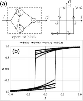
(a) Realization of an elementary hysteresis operator via a two-node DHNN [13], and (b) HHNN implementation of smooth hysteresis operators with 2kd = 0.48 [19].

According to the gradient descent rule, the output of say node A is changed as follows:

$$U_A(t+1)=\mathit{fd}({\mathit{net}}_A(t))\text{,}{\mathit{net}}_A(t)={\mathit{kU}}_B(t)+I\text{.}$$ (7)

The activation function, fd(x), is the signum function where:

$$\mathit{fd}(x)=\left\{\begin{array}{cc}+1\hfill & \text{if x}>0\hfill \\ -1\hfill & \text{if x}<0\hfill \\ \text{unchanged}\hfill & \text{if x}=0\hfill \end{array}.\right)$$ (8)

Obviously, a similar update rule is used for node B.

Assuming that k is positive and using the aforementioned update rules, the behavior of each of the outputs U_A and U_B follows the rectangular loop shown in Fig. 2a. The final output of the operator block, O, is obtained by averaging the two identical outputs hence producing the same rectangular loop.

It should be pointed out that the loop width may be controlled by the positive feedback weight, k. Moreover, the loop center can be shifted with respect to the x-axis by introducing an offset Q to its external input, I. In other words, the switching up and down values become equivalent to (Q + k) and (Q − k), respectively.

Hybrid Hopfield Neural Networks (HHNN)

Consider a general two-node HNN with positive feedback weights as shown in Fig. 2a. Whether the HNN is continuous or discrete, the energy function may be expressed by (6). Following the gradient descent rule for the discrete case, the output of, say, node A is changed as given by (7). Using the same gradient descent rule for the continuous case, the output is changed gradually as given by (4). More specifically, the output of, say, node A in the 2-node CHNN is changed as follows:

$$\frac{\partial U_A}{\partial t}=\eta \mathit{fc}({\mathit{net}}_A(t))\text{,}{\mathit{net}}_A(t)={\mathit{kU}}_B(t)+I\text{.}$$ (9)

While a CHNN will result in a single-valued input–output relation, a DHNN will result in the primitive rectangular hysteresis operator. The non-smooth nature of this rectangular building block suggests that a realistic simulation of a typical magnetic material hysteretic property will require a superposition of a relatively large number of those blocks. In order to obtain a smoother operator, a new hybrid activation function has been introduced in [19]. More specifically, the new activation function is expressed as:

$$f(x)=\mathit{cfc}(x)+\mathit{dfd}(x)\text{,}$$ (10)

where c and d are two positive constants such that c + d = 1 and fc and fd are given by (5) and (8), respectively.

The function f(x) is piecewise continuous with a single discontinuity at the origin. The choice of the two constants, c and d, controls the slopes with which the function asymptotically approaches the saturation values of −1 and 1. In this case, the new hybrid activation rule for, say, node A becomes:

$$U_A(t+1)=\mathit{cfc}({\mathit{net}}_A(t))+\mathit{dfd}({\mathit{net}}_A(t))\text{,}$$ (11)

where net_A(t) is defined as before. Fig. 2b depicts the smooth hyteresis operator resulting from the two-node HHNN. The figure illustrates how the hybrid activation function results in smooth Stoner–Wohlfarth-like hysteresis operators with controllable loop width and squareness [20]. In particular, within this implementation the loop width is equivalent to the product 2kd while the squareness is controlled by the ratio c/d. The operators shown in Fig. 2b maintain a constant loop width of 0.48 because k is set to (0.48/2d) for all curves [19].

Linear Neural Networks (LNN)

Given different sets of inputs I_i, i = 1, … , N and the corresponding outputs O, the linear neuron in Fig. 3a finds the weight values W₁ through W_N such that the mean-square error is minimized [13–16]. In order to determine the appropriate values of the weights, training data is provided to the network and the least-mean-square (LMS) algorithm is applied to the linear neuron. Within the training session, the error signal may be expressed as:

$$e(t)=O(t)-I^T(t)\mathbf{W}(t)\text{,}$$ (12)

where $\mathbf{W}={[W_1{W}_2\dots W_N]}^T\text{and}I={[I_1{I}_2\dots I_N]}^T$.

Fig. 3.

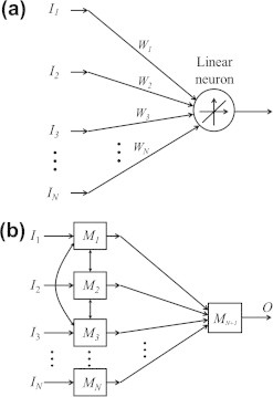
(a) A LNN, and (b) hierarchically organized MNN.

The LMS algorithm is based on the use of instantaneous values for the cost function: 0.5e²(t). Differentiating the cost function with respect to the weight vector W and using a gradient descent rule, the LMS algorithm may hence be formulated as follows:

$$\mathbf{W}(t+1)=\mathbf{W}(t)+\eta I(t)e(t)\text{,}$$ (13)

where η is the learning rate. By assigning a small value to η, the adaptive process slowly progresses and more of the past data is remembered by the LMS algorithm, resulting in a more accurate operation. That is, the inverse of the learning rate is a measure of the memory of the LMS algorithm [21].

It should be pointed out that the LNN and its LMS training algorithm are usually chosen for simplicity and user convenience reasons. Using any available software for neural networks, it is possible to utilize the LNN approach with little effort. However, the primary limitation of the LMS algorithm is its slow rate of convergence. Due to the fact that minimizing the mean square error is a standard non-linear optimization problem, there are more powerful methods that can solve this problem. For example, the Levenberg–Marquardt optimization method [22,23] can converge more rapidly than a LNN realization. In this method, the weights are obtained through the equation:

$$\mathbf{W}(t+1)=\mathbf{W}(t)+{({\mathit{\chi }}^T\mathit{\chi }+\delta \mathfrak{I})}^{-1}{\mathit{\chi }}^{T}e(t)\text{,}$$ (14)

where δ is a small positive constant, χ^T is a matrix whose columns correspond to the different input vectors I of the training data, and $\mathfrak{I}$ is the identity matrix.

Modular Neural Networks (MNN)

Finally, many electromagnetic problems are best solved using neural networks consisting of several modules with sparse interconnections between the modules [11–14,16]. Modularity allows solving small tasks separately using small neural network modules and then combining those modules in a logical manner. Fig. 3b shows a sample hierarchically organized MNN, which has been used in some electromagnetic applications [13].

Utilizing neural networks in modeling complex magnetic media

Restricting the focus on magnetization aspects of a particular material, complexity is usually defined by the permeability classification. For the case of complex magnetic materials, magnetization versus field (i.e., M–H) relations are nonlinear and history-dependent. Moreover, the vector M–H behavior for such materials could be anisotropic or even more complicated in nature. Whether the purpose is modeling magnetization processes or performing field computation within these materials, hysteresis models become indispensable. Although several efforts have been performed in the past to develop hysteresis models (see, for instance, [24–28]), the Preisach model (PM) emerged as the most practical one due to its well defined procedure for fitting its unknowns as well as its simple numerical implementation.

In mathematical form, the scalar classical PM [24] can be expressed as:

$$F(t)={\iint }_{\alpha ⩾\beta }\mu (\alpha \text{,}\beta ){\hat{\gamma }}_{\alpha \beta }u(t)d\alpha d\beta \text{,}$$ (15)

where f(t) is the model output at time t, u(t) is the model input at time t, while ${\hat{\gamma }}_{\alpha \beta }$ are elementary rectangular hysteresis operators with α and β being the up and down switching values, respectively. In (15), function μ(α, β) represents the only model unknown which has to be determined from some experimental data. It is worth pointing out here that such a hysteresis model can be physically constructed from an assembly of Schmidt triggers having different switching up and down values.

It can be shown that the model unknown μ(α, β) can be correlated to an auxiliary function F(α, β) in accordance with the expressions:

$$\mu (\alpha \text{,}\beta )=-\frac{{\partial }^{2}F(\alpha \text{,}\beta )}{\partial \alpha \partial \beta }\text{,}F(\alpha \text{,}\beta )=\frac{1}{2}(f_{\alpha }-f_{\alpha \beta })\text{,}$$ (16)

where f_α is the measured output when the input is monotonically increased from a very large negative value up to the value α, f_αβ is the measured output along the first-order-reversal curve traced when the input is monotonically decreased after reaching the value f_α [24].

Hence, the nature of the identification process suggests that, given only the measured first-order-reversal curves, the classical scalar PM is expected to predict outputs corresponding to any input variations resulting in tracing higher-order reversal curves. It should be pointed out that an ANN block has been used, with considerable success, to provide some optimum corrective stage for outputs of scalar classical PM [3].

Some approaches on utilizing ANNs in modeling magnetic media have been previously reported [29–36]. Nafalski et al. [37] suggested using ANN as an entire substitute to hysteresis models. Saliah and Lowther [38] also used ANN in the identification of the model proposed in Vajda and Della Torre [39] by trying to find its few unknown parameters such as squareness, coercivity and zero field reversible susceptibility. However, a method for solving the identification problem of the scalar classical PM using ANNs has been introduced [4]. In this approach, structural similarities between PM and ANNs have been deduced and utilized. More specifically, outputs of elementary hysteresis operators were taken as inputs to a two-layer FFNN (see Fig. 4a). Within this approach, expression (15) was reasonably approximated by a finite superposition of different rectangular operators as:

$$f(t)\approx {\displaystyle \sum _{i=1}^N}{\displaystyle \sum _{j=1}^N}\mu ({\alpha }_i\text{,}{\beta }_j){\hat{\gamma }}_{{\alpha }_i{\beta }_j}u(t)\text{,}{\alpha }_i={\beta }_i={\alpha }_1-2\frac{(i-1)}{(N-1)}{\alpha }_1\text{,}$$ (17)

where N² is the total number of hysteresis operators involved, while α₁ represents the input at which positive saturation of the actual magnetization curve is achieved.

Fig. 4.

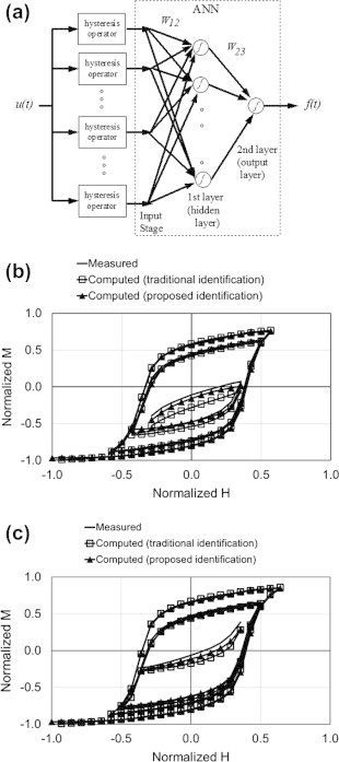
(a) Operator-ANN realization of the scalar classical PM, (b and c) comparison between measured data and model predictions based on both the proposed and traditional identification approaches [4].

Using selective and, supposedly, representative measured data, the network was then trained as discussed in the overview section. As a result, model unknowns were found. Obviously, choosing the proper parameters could have an effect on the training process duration. Sample training and testing results are given in Fig. 4b and c. It should be pointed out that similar approaches have also been suggested [40,41].

The ANN applicability to vector PM has been also extended successfully. For the case of vector hysteresis, the model should be capable of mimicking rotational properties, orthogonal correlation properties, in addition to scalar properties. As previously reported [7], a possible formulation of the vector PM may be given by:

$$\left[\begin{array}{c}{M}_x(t)\hfill \\ M_y(t)\hfill \end{array}\right]=\left[\begin{array}{c}{\iint }_{\alpha ⩾\beta }\left\{{\int }_{-\pi /2}^{+\pi /2}\cos \phi {\nu }_x(\alpha \text{,}\beta )f_x(\phi ){\hat{\gamma }}_{\alpha \beta }[{\overline{e}}_{\phi }·\bar{H}(t)]d\phi \right\}d\alpha d\beta \hfill \\ {\iint }_{\alpha ⩾\beta }\left\{{\int }_{-\pi /2}^{+\pi /2}\sin \phi {\nu }_y(\alpha \text{,}\beta )f_y(\phi ){\hat{\gamma }}_{\alpha \beta }[{\overline{e}}_{\phi }·\bar{H}(t)]d\phi \right\}d\alpha d\beta \hfill \end{array}\right]\text{,}$$ (18)

where ${\overline{e}}_{\phi }$ is a unit vector along the direction specified by the polar angle φ while functions ν_x, ν_y and even functions f_x, f_y represent the model unknowns that have to be determined through the identification process.

Substituting the approximate Fourier expansion formulations; f_x(φ) ≈ f_x0 + f_x1cos φ, and f_y(φ) ≈ f_y0 + f_y1cos φ in (18), we get:

$$\begin{array}{c}\hfill \left[\begin{array}{c}\hfill M_x(t)\hfill \\ \hfill M_y(t)\hfill \\ \hfill \hfill \end{array}\right]\approx \left[\begin{array}{c}\hfill {\displaystyle \sum _{{\alpha }_i⩾{\beta }_j}}{\nu }_{x0}({\alpha }_i\text{,}{\beta }_j){\mathit{Sx}}_{{\alpha }_i{\beta }_j}^{(0)}+{\displaystyle \sum _{{\alpha }_i⩾{\beta }_j}}{\nu }_{x1}({\alpha }_i\text{,}{\beta }_j){\mathit{Sx}}_{{\alpha }_i{\beta }_j}^{(1)}\hfill \\ \hfill {\displaystyle \sum _{{\alpha }_i⩾{\beta }_j}}{\nu }_{y0}({\alpha }_i\text{,}{\beta }_j){\mathit{Sy}}_{{\alpha }_i{\beta }_j}^{(0)}+{\displaystyle \sum _{{\alpha }_i⩾{\beta }_j}}{\nu }_{y1}({\alpha }_i\text{,}{\beta }_j){\mathit{Sy}}_{{\alpha }_i{\beta }_j}^{(1)}\hfill \\ \hfill \hfill \end{array}\right]\text{,}\hfill \end{array}$$ (19)

$${\nu }_{\omega 0}(\alpha \text{,}\beta )=f_{\omega 0}{\nu }_{\omega }(\alpha \text{,}\beta )\text{,}{\nu }_{\omega 1}(\alpha \text{,}\beta )=f_{\omega 1}{\nu }_{\omega }(\alpha \text{,}\beta )\text{,}\omega =x\text{,}y\text{,}$$ (20)

where

$$\begin{array}{c}\hfill \left[\begin{array}{c}\hfill {\mathit{Sx}}_{{\alpha }_i{\beta }_j}^{(0)}\hfill \\ \hfill {\mathit{Sx}}_{{\alpha }_i{\beta }_j}^{(1)}\hfill \\ \hfill {\mathit{Sy}}_{{\alpha }_i{\beta }_j}^{(0)}\hfill \\ \hfill {\mathit{Sy}}_{{\alpha }_i{\beta }_j}^{(1)}\hfill \end{array}\right]\approx \left[\begin{array}{c}\hfill \left\{{\displaystyle \sum _{n=1}^N}\cos {\phi }_n{\hat{\gamma }}_{{\alpha }_i{\beta }_j}[{\overline{e}}_{{\phi }_n}·\bar{H}(t)]\mathrm{\Delta }\phi \right\}\mathrm{\Delta }\alpha \mathrm{\Delta }\beta \hfill \\ \hfill \left\{{\displaystyle \sum _{n=1}^N}{\cos }^2{\phi }_n{\hat{\gamma }}_{{\alpha }_i{\beta }_j}[{\overline{e}}_{{\phi }_n}·\bar{H}(t)]\mathrm{\Delta }\phi \right\}\mathrm{\Delta }\alpha \mathrm{\Delta }\beta \hfill \\ \hfill \left\{{\displaystyle \sum _{n=1}^N}\sin {\phi }_n{\hat{\gamma }}_{{\alpha }_i{\beta }_j}[{\overline{e}}_{{\phi }_n}·\bar{H}(t)]\mathrm{\Delta }\phi \right\}\mathrm{\Delta }\alpha \mathrm{\Delta }\beta \hfill \\ \hfill \left\{{\displaystyle \sum _{n=1}^N}\frac{\sin 2{\phi }_n}{2}{\hat{\gamma }}_{{\alpha }_i{\beta }_j}[{\overline{e}}_{{\phi }_n}·\bar{H}(t)]\mathrm{\Delta }\phi \right\}\mathrm{\Delta }\alpha \mathrm{\Delta }\beta \hfill \end{array}\right]\text{,}\hfill \end{array}$$ (21)

$${\phi }_n=-\frac{\pi }{2}+\left(n-\frac{1}{2}\right)\mathrm{\Delta }\phi \text{,}\text{and}\mathrm{\Delta }\phi =\frac{\pi }{N}\text{.}$$ (22)

The identification problem reduces in this case to the determination of the unknowns ν_x0, ν_x1, ν_y0 and ν_y1. The FFNN shown in Fig. 5a has been used successfully to carry out the identification process by adopting the algorithms and methodologies stated in the overview section. Sample results of the identification process as well as comparison between predicted and measured rotational magnetization phase lag δ with respect to the rotational field component are given in Fig. 5b and c, respectively.

Fig. 5.

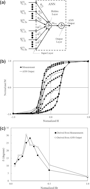
(a) The ANN configuration used in the model identification, (b) sample normalized measured and ANN computed first-order-reversal curves involved in the identification process, and (c) sample measured and predicted Hr − δ values.

Development of a computationally efficient vector hysteresis model was introduced based upon the idea reported [13] and presented in the overview section in which an elementary hysteresis operator was implemented using a two-node DHNN (please refer to Fig. 2a). More specifically, an efficient vector PM was constructed from only two scalar models having orthogonally inter-related elementary operators was proposed [14]. Such model was implemented via a LNN fed from a four-node DHNN blocks having step activation functions as shown in Fig. 6a. In this DHNN, the outputs of nodes A_x and B_x can mimic the output of an elementary hysteresis operator whose input and output coincide with the x-axis. Likewise, outputs of nodes A_y and B_y can represent the output of an elementary hysteresis operator whose input and output coincide with the y-axis. Symbols k_⊥, I_x and I_y are used to denote the feedback between nodes corresponding to different axes, the applied input along the x- and y-directions, respectively. Moreover, Q_i and k_//i are offset and feedback factors corresponding to the ith-DHNN block and given by:

$$Q_i=-\left(\frac{{\alpha }_i+{\beta }_i}{2}\right)\text{and}{k}_{//i}=\left(\frac{{\alpha }_i-{\beta }_i}{2}\right)\text{.}$$ (23)

Fig. 6.

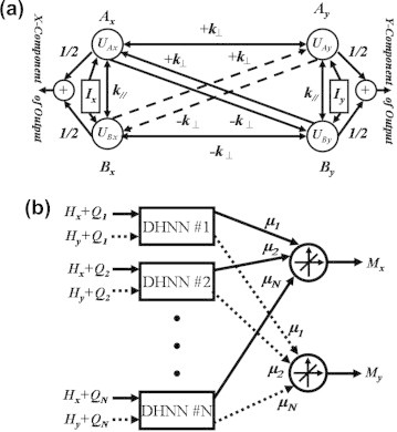
(a) A four-node DHNN capable of realizing two elementary hysteresis operator corresponding to the x- and y-axes, and (b) suggested implementation of the vector PM using a modular DHNN–LNN combination [14].

The state of this network converges to the minimum of the following energy function:

$$E=-\left[I_x(U_{\mathit{Ax}}+U_{\mathit{Bx}})+I_y(U_{\mathit{Ay}}+U_{\mathit{By}})+k_{//}{U}_{\mathit{Ax}}{U}_{\mathit{Bx}}+k_{//}{U}_{\mathit{Ay}}{U}_{\mathit{By}}+\frac{k_{\perp }}{2}(U_{\mathit{Ax}}-U_{\mathit{Bx}})(U_{\mathit{Ay}}+U_{\mathit{By}})+\frac{k_{\perp }}{2}(U_{\mathit{Ay}}-U_{\mathit{By}})(U_{\mathit{Ax}}+U_{\mathit{Bx}})\right]\text{.}$$ (24)

Similar to expressions (6)–(8) in the overview section, the gradient descent rule suggests that outputs of nodes A_x, B_x, A_y and B_y are changed according to:

$$\left[\begin{array}{c}\hfill U_{\mathit{Ax}}(t+1)\hfill \\ \hfill U_{\mathit{Bx}}(t+1)\hfill \\ \hfill U_{\mathit{Ay}}(t+1)\hfill \\ \hfill U_{\mathit{By}}(t+1)\hfill \\ \hfill \hfill \end{array}\right]=\left[\begin{array}{c}\hfill \text{sgn}(+k_{\perp }[U_{\mathit{Ay}}(t)+U_{\mathit{By}}(t)]+k_{//}{U}_{\mathit{Bx}}(t)+I_x)\hfill \\ \hfill \text{sgn}(-k_{\perp }[U_{\mathit{Ay}}(t)+U_{\mathit{By}}(t)]+k_{//}{U}_{\mathit{Ax}}(t)+I_x)\hfill \\ \hfill \text{sgn}(+k_{\perp }[U_{\mathit{Ax}}(t)+U_{\mathit{Bx}}(t)]+k_{//}{U}_{\mathit{By}}(t)+I_y)\hfill \\ \hfill \text{sgn}(-k_{\perp }[U_{\mathit{Ax}}(t)+U_{\mathit{Bx}}(t)]+k_{//}{U}_{\mathit{Ay}}(t)+I_y)\hfill \end{array}\right]\text{.}$$ (25)

Considering a finite number N of elementary operators, the modular DHNN of Fig. 6b. evolves – as a result of any applied input – by changing output values (states) of the operator blocks. Eventually, the network converges to a minimum of the quadratic energy function given by:

$$E=-{\displaystyle \sum _{i=1}^N}\left\{+\left(H_x-\left[\frac{{\alpha }_i+{\beta }_i}{2}\right]\right)(U_{\mathit{Axi}}+U_{\mathit{Bxi}})+\left(H_y-\left[\frac{{\alpha }_i+{\beta }_i}{2}\right]\right)(U_{\mathit{Ayi}}+U_{\mathit{Byi}})+\left[\frac{{\alpha }_i-{\beta }_i}{2}\right]U_{\mathit{Axi}}{U}_{\mathit{Bxi}}+\left[\frac{{\alpha }_i-{\beta }_i}{2}\right]U_{\mathit{Ayi}}{U}_{\mathit{Byi}}+\frac{k_{\perp }}{2}(U_{\mathit{Axi}}-U_{\mathit{Bxi}})(U_{\mathit{Ayi}}+U_{\mathit{Byi}})+\frac{k_{\perp }}{2}(U_{\mathit{Ayi}}-U_{\mathit{Byi}})(U_{\mathit{Axi}}+U_{\mathit{Bxi}})\right\}\text{.}$$ (26)

Overall output vector of the network may be expressed as:

$$M_x+{\mathit{jM}}_y={\displaystyle \sum _{i=1}^N}{\mu }_i\left[\left(\frac{U_{\mathit{Axi}}+U_{\mathit{Bxi}}}{2}\right)+j\left(\frac{U_{\mathit{Ayi}}+U_{\mathit{Byi}}}{2}\right)\right]\text{.}$$ (27)

Being realized by the pre-described DHNN–LNN configuration, it was possible to carry out the vector PM identification process using automated training algorithm. This gave the opportunity of performing the model identification using any available set of scalar and vector data. The identification process was carried out by first assuming some k_⊥i/k_//i ratios and finding out appropriate values for the unknowns μ_i. Training of the LNN was carried out to determine appropriate μ_i values using the available scalar data provided as explained in the overview section and as indicated by expression (13). Following the scalar data training process, available vector training data was utilized by checking best matching orthogonal to parallel coupling (k_⊥i/k_//i) for best overall scalar and vector training data match. Sample identification and testing results are shown in Fig. 7 (please refer to [14]). The approach was further generalized by using HHNN as described in the overview section [19]. Based upon this generalization and referring to (10) and (11), expression (25) is re-adjusted to the form:

$$\left[\begin{array}{c}\hfill U_{\mathit{Ax}}(t+1)\hfill \\ \hfill U_{\mathit{Bx}}(t+1)\hfill \\ \hfill U_{\mathit{Ay}}(t+1)\hfill \\ \hfill U_{\mathit{By}}(t+1)\hfill \end{array}\right]=\left[\begin{array}{c}\hfill \mathit{cfc}({\mathit{net}}_{\mathit{Ax}}(t))+\mathit{dfd}({\mathit{net}}_{\mathit{Ax}}(t))\hfill \\ \hfill \mathit{cfc}({\mathit{net}}_{\mathit{Bx}}(t))+\mathit{dfd}({\mathit{net}}_{\mathit{Bx}}(t))\hfill \\ \hfill \mathit{cfc}({\mathit{net}}_{\mathit{Ay}}(t))+\mathit{dfd}({\mathit{net}}_{\mathit{Ay}}(t))\hfill \\ \hfill \mathit{cfc}({\mathit{net}}_{\mathit{By}}(t))+\mathit{dfd}({\mathit{net}}_{\mathit{By}}(t))\hfill \\ \hfill \hfill \end{array}\right]\text{,}$$ (28)

where

$$\left[\begin{array}{c}\hfill {\mathit{net}}_{\mathit{Ax}}(t)\hfill \\ \hfill {\mathit{net}}_{\mathit{Bx}}(t)\hfill \\ \hfill {\mathit{net}}_{\mathit{Ay}}(t)\hfill \\ \hfill {\mathit{net}}_{\mathit{By}}(t)\hfill \end{array}\right]=\left[\begin{array}{c}\hfill \mathit{Ix}+{\mathit{kU}}_{\mathit{Bx}}(t)+\mathit{kc}(U_{\mathit{Ay}}(t)+U_{\mathit{By}}(t))\hfill \\ \hfill \mathit{Ix}+{\mathit{kU}}_{\mathit{Ax}}(t)-\mathit{kc}(U_{\mathit{Ay}}(t)+U_{\mathit{By}}(t))\hfill \\ \hfill \mathit{Iy}+{\mathit{kU}}_{\mathit{By}}(t)+\mathit{kc}(U_{\mathit{Ax}}(t)+U_{\mathit{Bx}}(t))\hfill \\ \hfill \mathit{Iy}+{\mathit{kU}}_{\mathit{Ay}}(t)-\mathit{kc}(U_{\mathit{Ax}}(t)+U_{\mathit{Bx}}(t))\hfill \end{array}\right]\text{.}$$ (29)

Fig. 7.

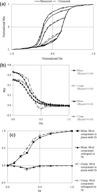
Comparison between measured and computed: (a) scalar training curves used in the identification process, (b) orthogonally correlated H_x–M_y data, and (c) rotational data, for k_⊥i/k_//i = 1.15 [14].

This generalization has resulted in an increase in the modeling computational efficiency (please refer to [19]).

Importance of developing vector hysteresis models is equally important for the case of anisotropic magnetic media which are being utilized in a wide variety of industries. Numerous efforts have been previously focused on the development of such anisotropic vector models (refer, for instance, to [24,42–46]). It should be pointed out here that the approach proposed by Adly and Abd-El-Hafiz [14] was further generalized [15] to fit the vector hysteresis modeling of anisotropic magnetic media. In this case the training process was carried out for both easy and hard axes data. Coupling factors were then identified to give best fit with rotational and/or energy loss measurements. Sample results of this generalization are shown in Fig. 8.

Fig. 8.

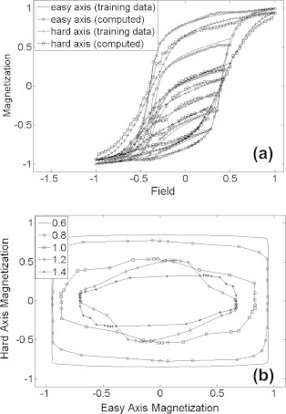
(a) Comparison between the given and computed normalized scalar data after the training process for Ampex-641 tape, and (b) sample normalized Ampex-641 tape vectorial output simulation results for different k_⊥ values corresponding to rotational applied input having normalized amplitude of 0.6 [15].

Another approach to model vector hysteresis using ANN was introduced [17,18] for both isotropic and anisotropic magnetic media. In this approach, a DHNN block composed of coupled N-nodes each having a step activation function whose output U ∊ {−1, +1} is used (please refer to Fig. 9a). Generalizing Eq. (6) in the overview section, the overall energy E of this DHNN may be given by:

$$E=-\bar{H}·{\displaystyle \sum _{i=1}^N}{U}_i{\overline{e}}_i-k_{\mathit{ij}}{\displaystyle \sum _{i=1}^N}{\displaystyle \sum _{{\displaystyle \genfrac{}{}{0ex}{}{j=1}{j\ne i}}}^N}(U_i{\overline{e}}_i·U_j{\overline{e}}_j)\text{,}\text{and}{k}_{\mathit{ij}}=\left\{\begin{array}{cc}\hfill -k_s\hfill & \hfill \text{for}{\overline{e}}_i·{\overline{e}}_j=-1\hfill \\ \hfill +k_m\hfill & \hfill \text{otherwise}\hfill \end{array}\right)$$ (30)

where $\overline{H}$ is the applied field, k_s is the self-coupling factor between any two step functions having opposite orientations, k_m is the mutual coupling factor, while U_i is the output of the ith step function oriented along the unit vector ${\overline{e}}_i$.

Fig. 9.

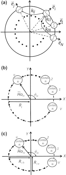
(a) DHNN comprised of coupled N-node step activation functions, (b) circularly dispersed ensemble of V similar DHNN, and (c) elliptically dispersed ensemble of V similar DHNN blocks [18].

According to this implementation, scalar and vectorial performance of the DHNN under consideration may be easily varied by simply changing k_s, k_m or even both. It was, thus, possible to construct a computationally efficient hysteresis model using a limited ensemble of vectorially dispersed DHNN blocks. While vectorial dispersion may be circular for isotropic media, an elliptical dispersion was suggested to extend the model applicability to anisotropic media. Hence, total input field applied to the uth DHNN block ${\overline{H}}_{\mathit{tu}}$ for the ith circularly and elliptically dispersed ensemble of V similar DHNN blocks (see Fig. 9b and c), may be respectively given by the expressions:

$${\bar{H}}_{\mathit{tu}}=\overline{H}+\overline{H}{o}_{\mathit{iu}}=\left\{\begin{array}{cc}\bar{H}+R_i{e}^{j{\phi }_{\mathit{iu}}}\hfill & \text{for isotropic case}\hfill \\ \bar{H}+\frac{e^{j{\phi }_{\mathit{iu}}}}{\sqrt{\frac{{\cos }^2{\phi }_{\mathit{iu}}}{R_{i-e}^2}+\frac{{\sin }^2{\phi }_{\mathit{iu}}}{R_{i-h}^2}}}\hfill & \text{for anisotropic case}\hfill \end{array}\right)$$ (31)

where ${\phi }_{\mathit{iu}}=\frac{2\pi }{V}(u-\frac{1}{2})$.

Using the proposed ANN configuration it was possible to construct a vector hysteresis model using only a total of 132 rectangular hysteresis operators which is an extremely small number in comparison to vector PMs. Identification was carried out for an isotropic floppy disk sample via a combination of four DHNN ensembles, each having N = V = 8, thus leading to a total of 12 unknowns (i.e., k_si, k_mi and R_i for every DHNN ensemble). Using a measured set of first-order reversals and measurements correlating orthogonal inputs and outputs, the particle swarm optimization algorithm was utilized to identify optimum values of the 12 model unknowns (see for instance [47]). Sample experimental testing results are shown in Fig. 10.

Fig. 10.

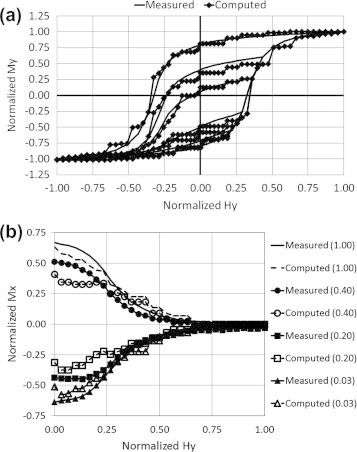
Comparison between computed and measured; (a) set of the easy axis first-order reversal curves, and (b) data correlating orthogonal input and output values (initial M_x values correspond to residual magnetization resulting from H_x values shown between parentheses) [18].

It was verified that 2D vector hysteresis models could be utilized in modeling 1D field-stress and field-temperature effects [48–50]. Consequently, it was possible to successfully utilize ANNs in the modeling of such coupled properties for complex magnetic media. For instance, in [13] a modular DHNN–LNN was utilized to model magnetization-strain variations as a result of field-stress variations (please see sample results in Fig. 11a and b). Similar results were also obtained in [16] using the previously discussed orthogonally coupled operators shown in Fig. 6. Likewise, modular DHNN-LNN was successfully utilized to model magnetization-field characteristics as a result of temperature variations [5] (please see sample results in Fig. 11c).

Fig. 11.

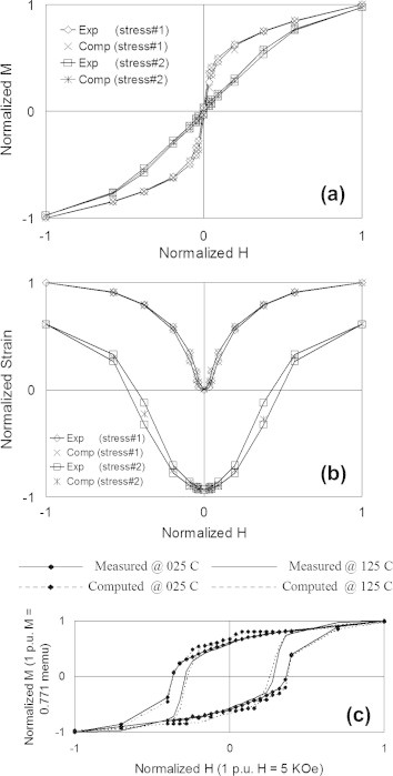
Measured and computed (a) M and (b) strain, for normalized H values and applied mechanical stresses of 0.9347 and 34.512 Kpsi [13], and (c) M–H curves for CoCrPt hard disk sample [5].

Utilizing neural networks in field computation involving nonlinear magnetic media

It is well known that field computation in magnetic media may be carried out using different analytical and numerical approaches. Obviously, numerical techniques become especially more appealing in case of problems involving complicated geometries and/or nonlinear magnetic media. In almost all numerical approaches, geometrical domain subdivision is usually performed and local magnetic quantities are sought (refer, for instance, to [51,52]). 2-D field computations may be carried out in nonlinear magnetic media using the automated integral equation approach proposed in Adly and Abd-El-Hafiz [11]. This represented a unique feature in comparison to previous HNN representations that dealt with linear media in 1-D problems (refer, for instance, to [9,53]).

According to the integral equation approach, field computation of the total local field values may be numerically expressed as [54–56]:

$$\bar{H}(q)=\bar{H}\mathit{app}(q)+\frac{1}{2\pi }{\displaystyle \sum _{i=1}^N}{\nabla }_q{\int }_{R_i}\overline{M}(p)·{\nabla }_p\ln (r_{\mathit{pq}}){\mathit{dS}}_p\text{,}$$ (32)

where N is the number of sub-region discretizations, q is an observation point, p is a source point at the center of the magnetic sub-region number i whose area is given by R_i, |r_pq| is the distance between points p and q while $\bar{H}$, ${\bar{H}}_{\mathit{app}}$ and $\bar{M}$ denote the total field, applied field and magnetization, respectively.

Solution of (32) is only obtained after a self-consistent magnetization distribution over all sub-regions is found, leading to an overall energy minimization as suggested by finite-element approaches. Assuming a constant magnetization within every sub-region, and taking magnetic property non-linearity into account, expression (32) may hence be re-written in the form:

$${\bar{H}}_i=\bar{H}{\mathit{app}}_i+{\displaystyle \sum _{j=1}^N}{\bar{C}}_{i\text{,}j}{\bar{M}}_j\left({\bar{H}}_j\right)\text{.}$$ (33)

where ${\bar{C}}_{i\text{,}j}$ is regarded as a geometrical coupling coefficient between the various sub-regions. In the particular case when i = j, ${\bar{C}}_{i\text{,}j}$ represents the ith sub-region demagnetization factor.

Since the M–H relation of most non-linear magnetic materials may be reasonably approximated by $\bar{M}\approx c\sqrt[n]{|\bar{H}|}{\overline{e}}_H$ [57], where n is an odd number, c is some constant and ${\overline{e}}_H$ is a unit vector along the field direction, this relation may be realized by a CHNN as shown in Fig. 12a. Since this single layer G-node fully connected CHNN should mimic a vectorial M–H relation, the G-nodes are assumed to represent a collection of scalar relations oriented along all possible 2-D directions. Hence:

$$\overline{m}={\displaystyle \sum _{k=1}^G}{\overline{e}}_{{\phi }_k}f(|\overline{h}|{\overline{e}}_h·{\overline{e}}_{{\phi }_k})\frac{\pi }{G}\text{,}f(h)=\mathit{ac}\sqrt[n]{h}\text{,}{\phi }_k=\left(k-\frac{1}{2}\right)\frac{\pi }{G}-\pi \text{,}$$ (34)

$$m\approx c\sqrt[n]{h}={\displaystyle \sum _{k=1}^G}\text{cos}{\phi }_{k}f(\mathit{hcos}{\phi }_k)\frac{\pi }{G}\Rightarrow \mathit{ac}=\frac{G}{\pi }\frac{c}{{\displaystyle \sum _{k=1}^G}{(\cos {\phi }_k)}^{\frac{1+n}{n}}}\text{,}$$ (35)

where ac is the activation function constant.

Fig. 12.

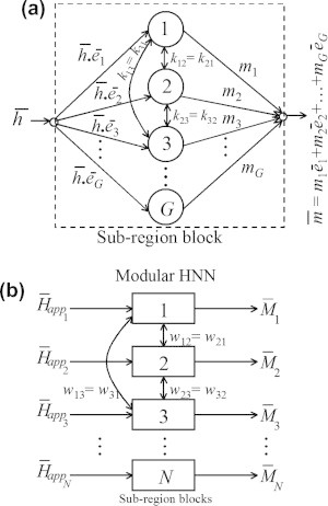
(a) Sub-region CHNN block representing vectorial M–H relation, and (b) integral equation representation using a modular CHNN, each block represents a sub-region in the discretization scheme.

The evolution of the network states is in the general direction of the negative gradient of any quadratic energy function of the form given in expression (2). A modular CHNN that includes ensembles of the CHNNs referred to as sub-region blocks was then used. Since each block represented a specific sub-region in the geometrical discretization scheme, it was possible to construct expression (33) as depicted in Fig. 12b. Evolution of this modular network followed the same reasoning described for individual sub-region blocks and, consequently, the output values converged based on the energy minimization criterion.

Verification of the presented methodology has been carried out [11] for nonlinear magnetic material as well as different geometrical and source configurations. Comparisons with finite-element analysis results have revealed both qualitative and quantitative agreement. Additional simulations using the same ANN field computation methodology have also been carried out [12] for an electromagnetic suspension system. Sample field computation results from [11,12] are shown in Fig. 13.

Fig. 13.

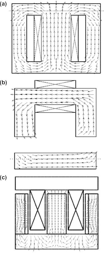
Flux density vector plot computed using the CHNN approach for; (a) a transformer, (b) an electromagnet, and (c) an electromagnetic suspension system [11,12].

It should be mentioned here that some evolutionary computation approaches – such as the particle swarm optimization (PSO) approach – has been successfully utilized as well for the field computation in nonlinear magnetic media (refer, for instance, to [58–61]). Nevertheless, in those approaches a discretization of the whole solution domain has to be carried out. This fact suggests that the presented CHNN methodology is expected to be computationally more efficient since it involves limited discretization of the magnetized parts only.

Discussion and conclusions

In this review article, examples of the successful utilization of ANNs in modeling as well as field computation involving complex magnetic materials have been presented. Those examples certainly reveal that integrating ANNs in some magnetics-related applications could result in a variety of advantages.

For the case of modeling complex magnetic media, DHNN as well as HHNN have been utilized in the construction of elementary hysteresis operators which represent the main building blocks of widely used hysteresis models such as the Preisach model. FFNN, LNN and MNN have been clearly utilized in constructing scalar, vector and coupled hysteresis models that take into account mechanical stress and temperature effects. The extremely important advantages of this ANN utilization include the ability to construct such models using any available mathematical software tool and the possibility of carrying out the model identification in an automated way and using any available set of training data.

Obviously, the presented different ANN implementations may be easily integrated in many commercially available field computation packages. This is especially an important issue knowing that most of those packages are not capable of handling hysteresis or coupled physical properties. Moreover, almost all implementations involving rectangular operators may be physically realized for real time control processes in the form of an ensemble of Schmitt triggers.

On the other hand, it was demonstrated that CHNN could be utilized in the field computation involving nonlinear magnetic media through linking the activation function to the media M–H relation. This has, again, resulted in the possibility to construct field computation tools using any available mathematical software tools and perform such computation in an automated way by the aid of built in HNN routines.

Finally, it should be stated that this review article may be regarded as a model for the wide opportunities to enhance; implementation, accuracy, and performance through interdisciplinary research capabilities.

Conflict of interest

The authors have declared no conflict of interest.

Compliance with Ethics Requirements

This article does not contain any studies with human or animal subjects.

Biographies

Amr A. Adly received the B.S. and M.Sc. degrees from Cairo University, Egypt, and the Ph.D. degree in electrical engineering from the University of Maryland, College Park in 1992. He also worked as a Magnetic Measurement Instrumentation Senior Scientist at LDJ Electronics, Michigan, during 1993–1994. Since 1994, he has been a faculty member in the Electrical Power and Machines Department, Faculty of Engineering, Cairo University, and was promoted to a Full Professor in 2004. He also worked in the United States as a Visiting Research Professor at the University of Maryland, College Park, during the summers of 1996–2000. He is a recipient of; the 1994 Egyptian State Encouragement Prize, the 2002 Shoman Foundation Arab Scientist Prize, the 2006 Egyptian State Excellence Prize and was awarded the IEEE Fellow status in 2011. His research interests include electromagnetic field computation, energy harvesting, applied superconductivity and electrical power engineering. Prof. Adly served as the Vice Dean of the Faculty of Engineering, Cairo University, in the period 2010-2014. Recently he has been appointed as the Executive Director of Egypt’s Science and Technology Development Fund.

Salwa K. Abd-El-Hafiz received the B.Sc. degree in Electronics and Communication Engineering from Cairo University, Egypt, in 1986 and the M.S. and Ph.D. degrees in Computer Science from the University of Maryland, College Park, Maryland, USA, in 1990 and 1994, respectively. Since 1994, she has been working as a Faculty Member at the Engineering Mathematics Dept., Faculty of Engineering, Cairo University, and has been promoted to a Full Professor at the same department in 2004. She co-authored one book, contributed one chapter to another book, and published more than 60 refereed papers. Her research interests include software engineering, computational intelligence, numerical analysis, chaos theory, and fractal geometry. Prof. Abd-El-Hafiz is a recipient of the 2001 Egyptian State Encouragement Prize in Engineering Sciences, recipient of the 2012 National Publications Excellence Award from the Egyptian Ministry of Higher Education, recipient of several international publications awards from Cairo University and an IEEE Senior Member.

References

- 1.Bozorth R. Wiley-IEEE Press; New Jersey: 1993. Ferromagnetism. [Google Scholar]
- 2.Mehrotra K., Mohan C.K., Ranka S. The MIT Press; Cambridge, MA: 1997. Elements of artificial neural networks. [Google Scholar]
- 3.Abd-El-Hafiz SK, Adly AA. A hybrid Preisach-neural network approach for modeling systems exhibiting hysteresis. In: Proceedings of the fourth IEEE international conference on electronics, circuits, and systems (ICECS’97), Cairo, Egypt; 1997. p. 976–9.
- 4.Adly A.A., Abd-El-Hafiz S.K. Using neural networks in the identification of Preisach-type hysteresis models. IEEE Trans Magn. 1998;34(3):629–635. [Google Scholar]
- 5.Adly A.A., Abd-El-Hafiz S.K., Mayergoyz I.D. Using neural networks in the identification of Preisach-type magnetostriction and field-temperature models. J Appl Phys. 1999;85(8):5211–5213. [Google Scholar]
- 6.Adly A.A., Abd-El-Hafiz S.K. Automated transformer design and core rewinding using neural networks. J Eng Appl Sci Facul Eng Cairo Univ. 1999;46(2):351–364. [Google Scholar]
- 7.Adly A.A., Abd-El-Hafiz S.K., Mayergoyz I.D. Identification of vector Preisach models from arbitrary measured data using neural networks. J Appl Phys. 2000;87(9):6821–6823. [Google Scholar]
- 8.Zurada J.M. West Publishing Company; St. Paul (MN): 1992. Introduction to artificial neural systems. [Google Scholar]
- 9.Adly A.A., Abd-El-Hafiz S.K. Utilizing Hopfield neural networks in the analysis of reluctance motors. IEEE Trans Magn. 2000;36(5):3147–3149. [Google Scholar]
- 10.Adly A.A., Abd-El-Hafiz S.K. Using neural and evolutionary computation techniques in the field computation of nonlinear media. Sci Bull Facul Eng Ain Shams Univ. 2003;38(4):777–794. [Google Scholar]
- 11.Adly A.A., Abd-El-Hafiz S.K. Automated two-dimensional field computation in nonlinear magnetic media using Hopfield neural networks. IEEE Trans Magn. 2002;38(5):2364–2366. [Google Scholar]
- 12.Adly AA, Abd-El-Hafiz SK. Active electromagnetic suspension system design using hybrid neural-swarm optimization. Proceedings of the 12th International Workshop on Optimization and Inverse Problems in Electromagnetism, Ghent, Belgium; 2012. p. 42-43.
- 13.Adly A.A., Abd-El-Hafiz S.K. Identification and testing of an efficient Hopfield neural network magnetostriction model. J Magn Magn Mater. 2003;263(3):301–306. [Google Scholar]
- 14.Adly A.A., Abd-El-Hafiz S.K. Efficient implementation of vector Preisach-type models using orthogonally-coupled hysteresis operators. IEEE Trans Magn. 2006;42(5):1518–1525. [Google Scholar]
- 15.Adly A.A., Abd-El-Hafiz S.K. Efficient implementation of anisotropic vector Preisach-type models using coupled step functions. IEEE Trans Magn. 2007;43(6):2962–2964. [Google Scholar]
- 16.Adly A.A., Abd-El-Hafiz S.K. Implementation of magnetostriction Preisach-type models using orthogonally-coupled hysteresis operators. Physica B. 2008;403:425–427. [Google Scholar]
- 17.Adly A.A., Abd-El-Hafiz S.K. Vector hysteresis modeling using octal clusters of coupled step functions. J Appl Phys. 2011;109(7) 07D342:1-3. [Google Scholar]
- 18.Adly A.A., Abd-El-Hafiz S.K. Efficient vector hysteresis modeling using rotationally coupled step functions. Physica B. 2012;407:1350–1353. [Google Scholar]
- 19.Adly A.A., Abd-El-Hafiz S.K. Efficient modeling of vector hysteresis using a novel Hopfield neural network implementation of Stoner–Wohlfarth-like operators. J Adv Res. 2013;4(4):403–409. doi: 10.1016/j.jare.2012.07.009. [DOI] [PMC free article] [PubMed] [Google Scholar]
- 20.Stoner E.C., Wohlfarth E.P. A mechanism of magnetic hysteresis in heterogeneous alloys. Proc Roy Soc A – Math Phys. 1948;240(826):599–642. [Google Scholar]
- 21.Haykin S. Prentice Hall; New Jersey: 1999. Neural networks: a comprehensive foundation. [Google Scholar]
- 22.Levenberg K. A method for the solution of certain problems in least squares. Q Appl Math. 1944;2:164–168. [Google Scholar]
- 23.Marquardt D. An algorithm for least-squares estimation of nonlinear parameters. SIAM J Appl Math. 1963;11(2):431–441. [Google Scholar]
- 24.Mayergoyz I.D. Elsevier Science Inc.; New York (NY): 2003. Mathematical models of hysteresis and their applications. [Google Scholar]
- 25.Mayergoyz I.D., Friedman G. Generalized Preisach model of hysteresis. IEEE Trans Magn. 1988;24(1):212–217. [Google Scholar]
- 26.Mayergoyz I.D., Friedman G., Salling C. Comparison of the classical and generalized Preisach hysteresis models with experiments. IEEE Trans Magn. 1989;25(5):3925–3927. [Google Scholar]
- 27.Mayergoyz I.D., Adly A.A., Friedman G. New Preisach-type models of hysteresis and their experimental testing. J Appl Phys. 1990;67(9):5373–5375. [Google Scholar]
- 28.Adly A.A., Mayergoyz I.D. Experimental testing of the average Preisach model of hysteresis. IEEE Trans Magn. 1992;28(5):2268–2270. [Google Scholar]
- 29.Del Vecchio P., Salvini A. Neural network and Fourier descriptor macromodeling dynamic hysteresis. IEEE Trans Magn. 2000;36(4):1246–1249. [Google Scholar]
- 30.Kuczmann M., Iványi A. A new neural-network-based scalar hysteresis model. IEEE Trans Magn. 2002;38(2):857–860. [Google Scholar]
- 31.Makaveev D., Dupré L., Melkebeek J. Neural-network-based approach to dynamic hysteresis for circular and elliptical magnetization in electrical steel sheet. IEEE Trans Magn. 2002;38(5):3189–3191. [Google Scholar]
- 32.Hilgert T., Vandevelde L., Melkebeek J. Neural-network-based model for dynamic hysteresis in the magnetostriction of electrical steel under sinusoidal induction. IEEE Trans Magn. 2007;43(8):3462–3466. [Google Scholar]
- 33.Laosiritaworn W., Laosiritaworn Y. Artificial neural network modeling of mean-field Ising hysteresis. IEEE Trans Magn. 2009;45(6):2644–2647. [Google Scholar]
- 34.Zhao Z., Liu F., Ho S.L., Fu W.N., Yan W. Modeling magnetic hysteresis under DC-biased magnetization using the neural network. IEEE Trans Magn. 2009;45(10):3958–3961. [Google Scholar]
- 35.Nouicer A., Nouicer E., Mahtali M., Feliachi M. A neural network modeling of stress behavior in nonlinear magnetostrictive materials. J Supercond Nov Magn. 2013;26(5):1489–1493. [Google Scholar]
- 36.Chen Y., Qiu J., Sun H. A hybrid model of Prandtl–Ishlinskii operator and neural network for hysteresis compensation in piezoelectric actuators. Int J Appl Electrom. 2013;41(3):335–347. [Google Scholar]
- 37.Nafalski A., Hoskins B.G., Kundu A., Doan T. The use of neural networks in describing magnetisation phenomena. J Magn Magn Mater. 1996;160:84–86. [Google Scholar]
- 38.Saliah H.H., Lowther D.A. The use of neural networks in magnetic hysteresis identification. Physica B. 1997;233(4):318–323. [Google Scholar]
- 39.Vajda F., Della Torre E. Identification of parameters in an accommodation model. IEEE Trans Magn. 1994;30(6):4371–4373. [Google Scholar]
- 40.Serpico C., Visone C. Magnetic hysteresis modeling via feed-forward neural networks. IEEE Trans Magn. 1998;34(3):623–628. [Google Scholar]
- 41.Visone C., Serpico C., Mayergoyz I.D., Huang M.W., Adly A.A. Neural–Preisach-type models and their application to the identification of magnetic hysteresis from noisy data. Physica B. 2000;275(1–3):223–227. [Google Scholar]
- 42.Di Napoli A., Paggi R. A model of anisotropic grain-oriented steel. IEEE Trans Magn. 1983;19(4):1557–1561. [Google Scholar]
- 43.Pfutzner H. Rotational magnetization and rotational losses of grain oriented silicon steel sheets-fundamental aspects and theory. IEEE Trans Magn. 1994;30(5):2802–2807. [Google Scholar]
- 44.Bergqvist A., Lundgren A., Engdahl G. Experimental testing of an anisotropic vector hysteresis model. IEEE Trans Magn. 1997;33(5):4152–4154. [Google Scholar]
- 45.Leite J., Sadowski N., Kuo-Peng P., Bastos J.P.A. Hysteresis modeling of anisotropic barium ferrite. IEEE Trans Magn. 2000;36(5):3357–3359. [Google Scholar]
- 46.Leite J., Sadowski N., Kuo-Peng P., Bastos J.P.A. A new anisotropic vector hysteresis model based on stop hysterons. IEEE Trans Magn. 2005;41(5):1500–1503. [Google Scholar]
- 47.Adly A.A., Abd-El-Hafiz S.K. Using the particle swarm evolutionary approach in shape optimization and field analysis of devices involving non-linear magnetic media. IEEE Trans Magn. 2006;42(10):3150–3152. [Google Scholar]
- 48.Adly A.A., Mayergoyz I.D. Magnetostriction simulation using anisotropic vector Preisach-type models. IEEE Trans Magn. 1996;32(5):4773–4775. [Google Scholar]
- 49.Adly A.A., Mayergoyz I.D., Bergqvist A. Utilizing anisotropic Preisach-type models in the accurate simulation of magnetostriction. IEEE Trans Magn. 1997;33(5):3931–3933. [Google Scholar]
- 50.Adly A.A., Mayergoyz I.D. Simulation of field-temperature effects in magnetic media using anisotropic Preisach models. IEEE Trans Magn. 1998;34(4):1264–1266. [Google Scholar]
- 51.Sykulski J.K. Chapman & Hall; London: 1995. Computational magnetics. [Google Scholar]
- 52.Chari M.V.K., Salon S.J. Academic Press; San Diego (CA): 2000. Numerical methods in electromagnetism. [Google Scholar]
- 53.Yamashita H., Kowata N., Cingoski V., Kaneda K. Direct solution method for finite element analysis using Hopfield neural network. IEEE Trans Magn. 1995;31(3):1964–1967. [Google Scholar]
- 54.Mayergoyz I.D. Naukova Dumka; Kiev, Ukraine: 1979. Iterative methods for calculations of static fields in inhomogeneous, anisotropic and nonlinear media. [Google Scholar]
- 55.Friedman G., Mayergoyz I.D. Computation of magnetic field in media with hysteresis. IEEE Trans Magn. 1989;25(5):3934–3936. [Google Scholar]
- 56.Adly A.A., Mayergoyz I.D., Gomez R.D., Burke E.R. Computation of fields in hysteretic media. IEEE Trans Magn. 1993;29(6):2380–2382. [Google Scholar]
- 57.Mayergoyz I.D., Abdel-Kader F.M., Emad F.P. On penetration of electromagnetic fields into nonlinear conducting ferromagnetic media. J Appl Phys. 1984;55(3):618–629. [Google Scholar]
- 58.Adly A.A., Abd-El-Hafiz S.K. Utilizing particle swarm optimization in the field computation of non-linear magnetic media. Appl Comput Electrom. 2003;18(3):202–209. [Google Scholar]
- 59.Adly A.A., Abd-El-Hafiz S.K. Field computation in non-linear magnetic media using particle swarm optimization. J Magn Magn Mater. 2004;272–276:690–692. [Google Scholar]
- 60.Adly A.A., Abd-El-Hafiz S.K. Speed range based optimization of non-linear electromagnetic braking systems. IEEE Trans Magn. 2007;43(6):2606–2608. [Google Scholar]
- 61.Adly A.A., Abd-El-Hafiz S.K. An evolutionary computation approach for time-harmonic field problems involving nonlinear magnetic media. J Appl Phys. 2001;109(7):07D321. [Google Scholar]