The Human Brain Encodes Event Frequencies While Forming Subjective Beliefs

Abstract

To make adaptive choices, humans need to estimate the probability of future events. Based on a Bayesian approach, it is assumed that probabilities are inferred by combining a priori, potentially subjective, knowledge with factual observations, but the precise neurobiological mechanism remains unknown. Here, we study whether neural encoding centers on subjective posterior probabilities, and data merely lead to updates of posteriors, or whether objective data are encoded separately alongside subjective knowledge. During fMRI, young adults acquired prior knowledge regarding uncertain events, repeatedly observed evidence in the form of stimuli, and estimated event probabilities. Participants combined prior knowledge with factual evidence using Bayesian principles. Expected reward inferred from prior knowledge was encoded in striatum. BOLD response in specific nodes of the default mode network (angular gyri, posterior cingulate, and medial prefrontal cortex) encoded the actual frequency of stimuli, unaffected by prior knowledge. In this network, activity increased with frequencies and thus reflected the accumulation of evidence. In contrast, Bayesian posterior probabilities, computed from prior knowledge and stimulus frequencies, were encoded in bilateral inferior frontal gyrus. Here activity increased for improbable events and thus signaled the violation of Bayesian predictions. Thus, subjective beliefs and stimulus frequencies were encoded in separate cortical regions. The advantage of such a separation is that objective evidence can be recombined with newly acquired knowledge when a reinterpretation of the evidence is called for. Overall this study reveals the coexistence in the brain of an experience-based system of inference and a knowledge-based system of inference.

Introduction

When facing a familiar environment, people rely on a priori knowledge to anticipate future events (Neisser, 1976; Bar, 2007). This ability develops in early childhood (Téglás et al., 2011). However, predictions often need to be adjusted when new observations are made because our knowledge about situations and people is often incomplete or biased (e.g., stereotypes). That is, our “internal model” of the world is only partial and objective evidence is needed to complete our beliefs.

Bayes' law provides a disciplined way to combine objective data with subjective prior beliefs. Behavioral studies have suggested that humans apply Bayesian principles when updating their knowledge (Peterson and Miller, 1965; Phillips and Edwards, 1966). Recent evidence has emerged in sensory decision making that uncertainty of prior knowledge relative to that of new data determines how posterior beliefs are formed, and neural signals of the corresponding uncertainty measures are beginning to be identified (Vilares et al., 2012). In the present study, we do not focus on the uncertainty of sensory information but on its probability of occurrence. Indeed, probabilities provide crucial information to predict what will happen next (d'Acremont and Bossaerts, 2012).

Both fMRI and EEG studies have shown that the brain response to uncertain stimuli depends on their actual frequency of occurrence. In the “odd ball” paradigm, a larger event-related potential (the P300) has been recorded for rare stimuli (Duncan-Johnson and Donchin, 1977; Mars et al., 2008). During reinforcement learning, authors have related BOLD activity in lateral parietal and prefrontal cortex to the occurrence of rare outcomes (Fletcher et al., 2001; Turner et al., 2004; Gläscher et al., 2010). Recently, it has been shown that the brain tracks the probability of up to 10 different stimuli in inferior parietal cortex and medial prefrontal cortex as well as their entropy in bilateral insula (d'Acremont et al., 2013). Missing, however, is a neurobiological account of how prior knowledge is merged with new factual evidence to form beliefs (Fig. 1).

Figure 1.

Illustration where a person intends to predict whether it will snow on Thursday. On Sunday night, the person watches a weather forecast, leading to the formation of a prior belief. During the next 3 d, the person observes factual weather information. On Monday and Tuesday it snows, but Wednesday is sunny. To make a prediction on Wednesday night, it is adaptive to take into account both the subjective prior information gathered from TV and the factual observations. It is unknown how the neural representation of this forecast integrates the prior knowledge with the actual frequency of experienced outcomes. Bayesian probabilities combine prior knowledge and empirical observations in an optimal way, whereas frequencies only depend on empirical observations.

Based on the literature and theoretical considerations, one can formulate several hypotheses. The first possibility is that regions previously found to react to likely (d'Acremont et al., 2013) or surprising events (Gläscher et al., 2010) do not incorporate prior knowledge when this factor is manipulated experimentally; thus these regions would encode stimulus frequencies. Another possibility is that BOLD signal in these regions incorporates prior knowledge. Such a result would support the Bayesian brain hypothesis. Bayes' rule does not require memory of past data, but only memory of the last forecast [like in the Kalman filter (Meinhold and Singpurwalla, 1983)]. Thus a neural signature of Bayesian probabilities does not necessitate the encoding of factual frequencies. A third scenario is that some of the regions found to be sensitive to stimulus probabilities in previous studies are specialized in encoding frequencies, while others incorporate prior knowledge in a Bayesian way. Our results favor the third hypothesis and point to the existence of a dual system of statistical inference in the brain.

Materials and Methods

Participants

Twenty-six participants took part in the study (11 women and 15 men). The median age was 23 years old (minimum, 18; maximum, 37). Twenty-four were students, graduate students, or postdoctorate students at the California Institute of Technology. Two were working outside of the college. The study took place at the Caltech Brain Imaging Center and was approved by the institutional review board.

Participants read the task instructions on the computer screen and practiced with two demonstration trials before the fMRI scanning. Participants began the session with $1 play money. The net payoff received in each trial was added to the play money. At the end of the experiment, they received four times the final play money in real currency (U.S. dollars). This variable amount was added to a fixed amount given for the participation in the study.

Task design

In our paradigm, participants were asked to estimate the probability of uncertain stimuli based on a priori information as well as repeated empirical observations. We tracked brain activity as evidence (stimuli) was accumulated. In our weather analogy (Fig. 1), evidence would correspond to the weather experienced each day. In addition, the reward associated with a stimulus was manipulated independently of its probability of occurrence, so the evidence was affectively neutral on average. In the weather analogy (Fig. 1), the decision maker might want to ski on Thursday. Thus “snow” would be a positively valued outcome. Conversely, he might need to drive, so that “snow” would be a bad outcome. The task thus introduced a distinction between objective and subjective probabilities while controlling for the effect of value.

Two novel tasks were developed to test the hypotheses presented in the introduction. The two tasks shared a common principle: participants received prior but incomplete information about the likelihood of observing two mutually exclusive stimuli. They later had the opportunity to refine their prediction after observing the factual occurrence of the stimuli. However, the causal model generating the stimuli differed between the two tasks. This strategy was followed to test the robustness of our findings and enhance the generality of the results.

Stimuli presented in the two tasks were distinguished by their color. In the first task, the ball betting task, prior information was given on the proportion of red and blue balls in a unique bin. Participants bet whether the ball drawn next would be of a designated color (red or blue; Fig. 2a). In the second task, the bin betting task, prior information was given on the probability that balls would be drawn from a designated bin (right or left). The two bins contained a different proportion of green and orange balls and participants bet whether ball drawings came from the designated bin (Fig. 2b). Participants were asked to bet on the ball/bin associated with the $1 payoff. In Figure 2 for instance, they had to bet on the red ball in the ball betting task and the right bin in the bin betting task. In half of the trials, the payoff was associated to the other ball/bin. With this design, stimulus probability and reward were statistically independent (see below, Randomization).

Figure 2.

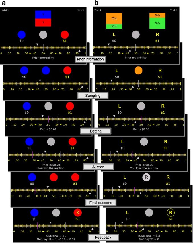
a, b, One trial of the ball betting task (a) and bin betting task (b). Prior information: the two gray triangles gave incomplete prior information on the probability of the rewarded ball (ball betting task) or the rewarded bin (bin betting task). Sampling: between one and nine balls were drawn with replacement and shown in the center of the screen. Betting: participants placed a bet by moving a vertical gray line on the scale. Auction: the computer selected a price at random and displayed it by moving a vertical violet line; the outcome of the auction was revealed simultaneously. Final outcome: an additional ball was drawn in the ball betting task and the bin was revealed in the bin betting task. Feedback: payoff and net payoff were displayed.

Each trial was divided into six periods. In the prior information period, a range of possible probability was revealed by moving two triangles on a horizontal scale. The computer chose a value p between the triangles (p was not revealed). In the ball betting task, p determined the true probability that a ball associated with the $1 payoff (Fig. 2a, red ball) would be drawn from the bin. In the bin betting task, p determined the true probability that balls came from a designated bin (Fig. 2b, right bin). In the sampling period, objective empirical evidence was generated by repeatedly drawing balls (with replacement). Between one and nine balls were drawn. To ensure that participants carefully attended to each drawing, we randomly ended the drawing in each trial. In the subsequent betting period, participants bet between $0 and $1 on the color of the next ball (in the ball betting task) or on the designated bin (in the bin betting task) by moving a vertical gray line along the horizontal scale (participants placed their bet at the end of the sampling period, not after each drawing). As indicated previously, the ball (red/blue) or bin (right/left) they bet on was the one associated with the $1 payoff.

After the bet was chosen, we ran a second price auction to determine payoffs. This method was selected because it incites participants to accurately report their estimation of probabilities (Becker et al., 1964). In the auction period, the computer revealed a price by moving a vertical violet bar between $0 and $1. Participants won the auction if the bet was strictly higher than this random price. If the bet was equal or smaller than the computer price, the auction was lost. In the final outcome period, an additional ball was drawn in the ball betting task and the bin was revealed in the bin betting task. The earning for the current trial was shown in the feedback period. In case the auction was won, the payoff was $1 if the additional ball drawn was of the designated color (ball betting task) or if the bin from which balls had been drawn was the designated one (bin betting task). Otherwise the payoff was zero. The net payoff equaled the payoff minus the computer drawn price. Net payoff could be negative. In case the auction was lost, the net payoff was always zero. At the end of the auction, the net payoff was added to the play money. The details of the auction made it optimal to place a bet equal to the probability to obtain the $1 payoff (see below, Predictive models for choices). To avoid errors due to a misunderstanding of the second price auction, the optimal strategy was made explicit in the task instruction.

Randomization

The value of p that determined the probability of the final outcome was chosen from a uniform distribution between the two triangles. To vary the uncertainty about the prior information, the distance d between the triangles changed from one trial to the other. In the ball betting task, the distance could be 0.25, 0.50, or 1. The computer selected one of the three possible distances with equal likelihood. The position of the triangles on the scale was determined by two values: a and b. The value a was chosen between 0 and 1 − d from a uniform distribution. The value b was defined as a + d.

In the bin betting task, the three possible distances between the triangles were 0, 0.25, and 0.50. Positions a and b of the triangles were determined as in the ball betting task. For the distance 0, the triangles were superimposed and determined the exact prior. Note that contrary to the bin betting task, the distance between the triangles was never zero in the ball betting task. Otherwise the proportion of balls in the (unique) urn would have been known exactly, obviating the need for learning.

There was at least one drawing in the sampling period. Subsequently, there was a 20% chance that the sampling would end after each drawing. The maximum number of drawings was nine. Thus the number of drawings ranged from one to nine.

Participants performed eight trials of the ball betting task, eight trials of the bin betting task, eight trials of ball betting task again, and eight trials of the bin betting task again. At the beginning of the session, the computer randomly chose whether participants started with eight trials of the ball betting task or eight trials of the bin betting task. Within a block of eight trials, the color–payoff association or the bin–payoff association changed after four trials. This way, the effect of stimulus value and probability could be dissociated. Whether the first block started with the red/right–payoff association or the blue/left–payoff association was chosen randomly at the beginning of each session.

Duration and message

Prior information.

The play money at the beginning of the task was $1. Messages were displayed on the bottom of the screen. Each trial started with a message “Total = X” showing the current play money (2.5 s). Then the message “Prior probability” was displayed (3.5 s). The gray triangles were moved to display the prior information. After 5.5 s, the message “Fill in the urn” for the ball betting task or “Select the urn” for the bin betting task was displayed (2 s).

Sampling.

The sampling period was announced with the message “Start sampling” (2 s). A fixation cross was flashed (0.2 s). Colored balls (stimuli) were shown in the middle of the screen for 1 s one after another. The interstimulus interval was drawn from a uniform distribution between 3 and 4 s (jittering).

Betting.

The betting period was announced with the message “Start auction” (3.5 s) followed by the message “Your bet on the ball?” for the ball betting task and “Your bet on the urn?” for the bin betting task. Participants had a maximum of 20 s to place their bet by moving a vertical gray line on a scale between $0 and $1. The position of the line was recorded after they clicked on the track ball button, or after the time limit was reached. A feedback message “Bet is X,” indicating the recorded bet, was displayed for 3.5 s.

Auction.

The auction period was announced with the message “Select price” (3.5 s). A vertical violet line was moved to reveal the computer price. At the same time, a message indicating the price “Price is X” and a message indicating whether the participant won the auction or not was displayed over 5.5 s.

Final outcome.

This period started with the message “Draw last ball” for the ball betting task and “Reveal the urn” for the bin betting task. A fixation cross was flashed (0.2 s) followed by an interstimulus interval (3–4 s). Then the color of the ball or the side of the bin was revealed in the center of the screen (1 s).

Feedback.

After an interstimulus interval (3–4 s), the payoff associated to the outcome “Outcome = X” and the net payoff “Net payoff = Y” were displayed for 5.5 s. Then a new trial started.

Predictive models for brain activity

We focus on brain activation correlating with the probability of occurrence of each type of stimulus, distinguishable by the color of the ball drawn from the bin (red or blue for the ball betting task; green or orange for the bin betting task). We measure stimulus probabilities in two ways. First, we compute probabilities ignoring prior information. Hence, these probabilities are purely based on the actual frequency of occurrence of the colors. We refer to this model as “frequentist.” Second, we use Bayesian posterior beliefs computed from the prior information and the history of sampling of colors. This model will be referred to as “Bayesian.” The naming is in no way meant to reflect arguments in the statistics literature on the relative merits of using prior information (Bayesian statistics) against considering only the objective information that could possibly emerge (classical frequentist statistics; Fienberg, 2006). Instead, it is a convenient way to distinguish between updating based on prior information and updating excluding prior information (Fig. 1).

Frequentist model.

In the frequentist model, we ignore the prior information; inference is solely based on the factual drawings. In the ball betting task, the probability of observing another red ball after recording k red balls in n prior draws is given by Equation 1:

The probability of a blue ball is the complementary of the probability of a red ball (mutually exclusive events). In the bin betting task, the probability of observing another green ball after recording k green balls in n prior draws is given by Equation 2:

The probability of an orange ball is the complementary probability.

Bayesian model.

The Bayesian model combines factual frequencies with prior knowledge. For the ball betting task, we provide a formula for the posterior probability that a red ball would be drawn conditional on the past draws and prior information (about the composition of the bin, delivered at the beginning of each trial). The random variables are the following: θ indicates the proportion of red balls in the bin, an outcome of the random variable ϴ; k is the outcome of a binomial random variable and denotes the number of red balls observed in n drawings.

At the beginning of each trial, ϴ follows a uniform distribution between [a, b], where a and b denote the positions of the triangles on the screen (0 < a < b < 1). The probability that ϴ takes the value θ equals the probability density function of the uniform distribution (we use the symbol P for both probability density and mass functions) as shown in Equation 3:

The probability of observing k red balls in n drawings given a certain proportion of red balls θ is given by the density function of the binomial distribution (0 ≤ k ≤ n), as shown in Equation 4:

The probability of observing another red ball after recording k red balls in n previous draws can be calculated with the Bayes' law, which gives in Equation 5 the following:

where Beta denotes the incomplete Beta function.

For the bin betting task, the Bayesian model provides the posterior probability that the right bin is used in the ball drawing. The probability that draws come from the left bin is complementary to that for the right bin (mutually exclusive events). We first define the relevant random variables. Let U denote a variable following a Bernoulli distribution with parameter θ indicating if the left (U = 0) or right (U = 1) bin was selected to draw balls. θ is the outcome of a random variable ϴ. k is a random variable following a binomial distribution indicating the number of green balls observed in n drawings. The parameter of this binomial distribution equaled three-tenths if the left bin was selected (U = 0) and seven-tenths if the right bin was selected (U = 1).

At the beginning of each trial, ϴ follows a uniform distribution between [a, b], with a and b given by the position of the triangles on the screen (0 < a < b < 1). The probability that ϴ takes the value θ equals the probability density function of the uniform distribution as shown in Equation 6:

The probability that the bin u (= 0, 1) is selected given θ equals the probability mass function of the Bernoulli distribution is as follows in Equation 7:

The probability of observing k green balls in n drawings given u (right or left bin) equals the probability density function of the binomial distribution (0 ≤ k ≤ n) as shown in Equation 8:

where R and L denote the probability of drawing a green ball when the right or left bin is selected, respectively.

To calculate the probability that the right bin was selected, given the observed data, we apply Bayes' rule, which in Equation 9 produces:

The probability of observing a green ball after sampling is given by the following Equation 10:

Predictive models for choices

Participants bet to earn a $1 payoff. It can be shown that the maximum expected net payoff is obtained when the bet b equals the probability p of receiving the payoff in the gamble (b = p). Thus, it is optimal to place a bet equal to the probability of winning the gamble. In case the bet is optimal, the expected net payoff is a quadratic function of the probability p, as shown in Equation 11:

In the behavioral analysis, we could have used statistical models that directly predicted the bet. However, risk aversion may bias such an approach. Specifically, risk-averse participants decrease their bet below their belief (of winning the gamble) to increase the chance to lose the auction and hence avoid the gamble altogether. Therefore, we ran analyses on an adjusted bet. When the red ball or right bin was rewarded, the adjusted bet equaled the observed bet (b); otherwise the adjusted bet was 1 minus the observed bet (1 − b). The effect of risk attitude then cancels out across the two conditions. For simplicity, we refer to the adjusted bet simply as “bet” or “inferred belief” in the sequel.

Frequentist model.

In the ball betting task, the bet was predicted by the frequency of the red ball (Eq. 1). In the bin betting task, participants bet on the bin, not the ball. Thus the bet was predicted by the probability that the right bin was selected conditional on the drawings and a Bayesian prior probability equal to $\frac{1}{2}$. This way, the prior information was effectively ignored in the model and behavioral response in the two tasks could be compared. The probability that the right bin was used to draw balls is given by the following Equation 12:

Bayesian model.

In the ball betting task, the bet was predicted by the red ball probability, calculated with Bayes' formula (Eq. 5). In the bin betting task, the bet was predicted by the probability that the right urn was the one used to draw balls, calculated with Bayes' formula (Eq. 9).

Behavioral analysis

Bets were predicted with mixed-linear models. Subject was entered as a random factor to capture individual variability. Mixed linear regressions were estimated in R with the lme function (R Development Core Team, 2012). See Predictive models for choices for details on the calculation of frequentis (Eqs. 1 and 12) and Bayesian probabilitie (Eqs. 5 and 9). The threshold for significance was set at p < 0.05.

Brain analysis

Image acquisition.

BOLD fMRI acquisitions were performed with a 32-channel head coil on a 3 T Siemens Tim-Trio system. Functional MRI images were acquired with an EPI gradient echo T2*-weighted sequence [flip angle, 80°; TR, 2000 ms; TE, 30 ms; 64 × 64 matrix, GRAPPA (generalized autocalibrating partially parallel acquisition) acceleration, 2; voxel size, 3 × 3 × 3 mm; 38 slices, covering the whole brain].

High resolution morphological data were acquired with a sagittal T1-weighted 3D magnetization prepared rapid acquisition gradient echo (MP/RAGE) sequence, 176 slices (with voxel size of 1 mm isotropic), as a structural basis for brain segmentation and surface reconstruction.

Preprocessing.

fMRI preprocessing steps, conducted with SPM8 (Wellcome Department of Cognitive Neurology, London, United Kingdom), included realignment of intrasession acquisitions to correct for head movement, normalization to a standard template [Montreal Neurological Institute template (MNI)] to minimize interparticipant morphological variability and resampling to isotropic voxel of 2 × 2 × 2 mm to improve superposition of functional results and morphological acquisitions, and convolution with an isotropic Gaussian kernel (FWHM, 6 mm) to increase signal-to-noise ratio. The signal drift across acquisitions was removed with high-pass filter (only signals with a period <240 s were included).

Voxel-based analysis.

Subject was defined as a random factor in general linear models (GLMs). GLMs were estimated with SPM8. The default orthogonalization of predictors was removed to avoid arbitrary results due to predictor order.

GLM events were defined for all messages displayed during the tasks. Event duration equaled the duration of the messages. In the prior information epoch, a GLM event was defined when the two triangles indicating prior information moved from their central positions. The event was modulated parametrically by the Bayesian expected net payoff calculated on condition of an optimal bet and with the use of the displayed prior information. The left-to-right position of the middle point between the triangles was defined as a second parametric modulator.

During the sampling period, GLM events were defined for the fixation cross, the interstimulus interval (gray ball), and the stimulus itself (drawing of a ball). The duration of these events in the GLM was equal to their duration in the tasks. The stimulus was modulated parametrically by the number of drawings (balls, regardless of color) since the beginning of the trial (1, 2, 3, etc.) and the frequency of occurrence of the color (color probability, GLM1). In a second GLM, Bayesian posterior probabilities substituted for frequencies to localize the neural representation of subjective beliefs (GLM2). In GLM1 and GLM2, BOLD activity was regressed on the probability of the currently observed stimulus. The probability of “red” (“blue”) was used when a red (blue) ball was drawn in the ball betting task. The probability of “green” (“orange”) was used when a green (orange) ball was drawn in the bin betting task. See Predictive models for brain activity for details on the calculation of frequentist (Eqs. 1 and 2) and Bayesian probabilities (Eqs. 5 and 10).

Update was substituted for probability as a parametric modulator to test whether the brain was encoding a change in belief based on the currently observed stimulus. The update was calculated as the posterior minus the prior (GLM3), or as the log of the ratio posterior/prior (GLM4). To test if probabilities were encoded differently depending on the task, the stimulus probability was modulated by the task identity (ball betting task, 0; bin betting task, 1; GLM5). To test the role of value, the stimulus was modulated by the Bayesian expected net payoff based on Equation 6 (GLM6). To further explore the effect of value, the stimulus was modulated by its associated payoff ($0 or $1) in a separate GLM (GLM7).

In the betting epoch of both tasks, a GLM event was defined for the time spent placing the bet. This event was modulated by the left-to-right position of the middle point between the triangles. A covariate was used to make the distinction between participants' placing their bet with the left (covariate, 0) or right hand (covariate, 1). In the auction epoch, the message display event was modulated parametrically by the content of the message; namely, the computer-generated price. In the feedback period, a GLM event was defined for the interstimulus interval (gray ball) that followed the revelation of the final outcome (color of the ball or side of the bin). This event was modulated by the net payoff.

Seven GLMs were estimated at this point: GLM1 (frequency), GLM2 (Bayesian probability), GLM3 (Bayesian update computed as a difference), GLM4 (Bayesian update computed as a ratio), GLM5 (task identity), GLM6 (Bayesian expected net payoff), and GLM7 (payoff). The appropriate GLM was selected when presenting results related to the stimulus displayed during the sampling period. Results for the remaining events were similar for the seven GLMs. We report the estimation found with GLM2 when presenting results not related to the stimulus. For voxel-based analyses (including identification of ROIs), the threshold for significance was set at p < 0.001, uncorrected, with minimal cluster size of 100 voxels. Coordinates are given in the MNI space (millimeters).

ROI analysis.

By definition, probabilities calculated with the frequentist and Bayesian models are both functions of the observed drawings. As a consequence, their correlation was relatively high (r = 0.66). To document their effect at the voxel level, a GLM was estimated separately for frequentist (GLM1) and Bayesian probabilities (GLM2). We should observe some overlap in brain activity as the two predictors share information. The key analysis was to estimate their unique contribution. To do so, frequentist and Bayesian probabilities were entered together in the same regression to explain the average BOLD effect found in a given ROI. This way, we directly contrasted the two explanatory variables (Poldrack et al., 2008).

ROIs encoding probabilities were defined by merging the voxels found to encode objective frequencies and Bayesian posterior probabilities. Voxels had to belong to GLM1 or GLM2 clusters of activation (or both). With this approach, none of the two types of probability was favored in the definition of the ROIs. To avoid circularity or “double dipping,” ROIs for each participant were determined based on the data of all other participants (Kriegeskorte et al., 2009).

The GLMs for the ROI analysis (GLM8) was the same as the GLMs for the voxel-based analysis (GLM1–GLM7), except that different events were defined for each drawing of a ball (stimuli) during the sampling period. These events were not modulated by covariates. GLM8 was fitted to the brain functional data and Marsbar toolbox was used to extract the first component score of all voxels in a given ROI (Brett et al., 2002). This was done for each subject separately. Because ROIs for each subject were estimated without the subject himself, circularity was avoided. Estimated βs were imported in R (R Development Core Team, 2012). In R, mixed linear regressions (lme function) were computed to predict the β estimated for each stimulus obtained from Marsbar. Consistent with the voxel-based GLMs, subject was defined as a random factor in R mixed linear regressions. The threshold was set to p < 0.05 when analyzing average activation in ROIs.

Connectivity analysis.

Functional connectivity was analyzed with the psychophysiological interaction (PPI) toolbox of SPM8. ROIs were used as seed regions. Connectivity in the sampling period was analyzed with a GLM fitted on images acquired during the sampling period (physiological factor). No experimental variable was included (psychological factor). As for all other voxel-based GLMs, connectivity analyses included realignment regressors to control for head motion (Weissenbacher et al., 2009). The high-pass filter was maintained at 240 s to allow the comparison of results obtained with the connectivity analyses and the other GLMs.

Results

Participant choices

Participant bets were first regressed on the Bayesian probabilities. Results showed that the slope (β) coefficients were close to 1 and highly significant in the ball betting task (β = 1.15, t₍₃₈₈₎ = 24.60, p < 0.001) as well as in the bin betting task (β = 0.82, t₍₃₈₈₎ = 22.64, p < 0.001). When probabilities based on the Bayesian and frequentist models were entered in the same regressions to explain bets, Bayesian probabilities remained significant in the ball and bin betting tasks (respectively β = 0.86, t₍₃₈₇₎ = 14.16, p < 0.001; β = 0.62, t₍₃₈₇₎ = 11.33, p < 0.001). The effect of objective frequencies was smaller but still significant in both tasks (β = 0.22, t₍₃₈₇₎ = 5.14, p < 0.001; β = 0.22, t₍₃₈₇₎ = 3.26, p = 0.001), indicating that participant beliefs were slightly biased by the factual stimulus frequencies away from full Bayesian posteriors (Fig. 3). Belief about the outcome was unaffected by its associated value ($0 or $1) in the two tasks (p = 0.92; p = 0.84). Thus values did not influence beliefs, a rational strategy because values were irrelevant to estimate outcome probabilities (Savage, 1954).

Figure 3.

Participant beliefs as a function of outcome probabilities. The following beliefs were inferred from bets: the belief that a red ball would be drawn (ball betting task) or that the right bin was used to draw balls (bin betting task). Outcome probabilities were calculated based on only the observed balls (frequentist) or computed by optimally integrating prior information with observed frequencies (Bayesian). A linear model was fit to beliefs with the two types of probabilities entered simultaneously as explanatory variables, as well as a dummy variable for condition (whether the red ball/right bin was associated with the $1 payoff). Heights of the bars represent t values (relative effect size). Dotted line indicates significance at p = 0.05.

When data of the two tasks were concatenated and a factor defining the task was created (ball betting task, 0; bin betting task, 1), the effect of Bayesian probabilities was greater (β = 0.86, t₍₇₉₉₎ = 14.05, p < 0.001) compared with frequencies (regardless of the task). Frequencies still had a significant effect on choices (β = 0.23, t₍₇₉₉₎ = 4.60, p < 0.001). The Bayesian probability–task interaction was significant (β = −0.23, t₍₇₉₉₎ = −2.92, p = 0.004), but the frequentist probability–task interaction was not (β = −0.01, t₍₇₉₉₎ = −0.16, p = 0.87). Overall, Bayesian probabilities better explained bets, suggesting that participants effectively took into account prior information when making predictions. Integrating prior information with observed evidence was more difficult in the bin betting task compared with the ball betting task.

Brain activation

Prior information epoch

At the beginning of a trial, the (prior) probability of receiving the $1 payoff was equal to the value of the point situated midway between the two triangles. The expected net payoff (payoff minus expected price) was a quadratic function of this probability (Eq. 11), provided that participants would place the optimal bet at the end of the trial.

Results showed significant activation in the occipital cortex related to the left–right position of the triangles on the screen. This indicates that participants were paying attention to the information provided at the beginning of the trial (Fig. 4a). When the triangles moved to the left side of the screen, more activation was observed in the left occipital cortex. This can be explained because the bin(s) in the center of the screen created more luminescence in the right visual field when participants looked to the left. Consistent with documented involvement of striatal regions in signaling expected rewards (O'Doherty et al., 2004), the expected net payoff was correlated with BOLD signal in left caudate (Fig. 5a).

Figure 4.

Visual and motor activation. a, BOLD response occipital cortex during the prior information period as a function of the left-to-right position of the triangles (ipsilateral activation). b, BOLD response in occipital cortex during the betting period as a function of the left-to-right position of the triangles (ipsilateral activation). c, BOLD response in primary motor cortex during the betting period as a function of the use of the left or right hand to place the bet (controlateral activation).

Figure 5.

Brain activation in striatum as a function of value. a, Activation during the prior information period in left caudate as a function of the expected net payoff based on the displayed information. b, BOLD response in bilateral caudate increased as the computer-generated price decreased in the auction epoch. c, Activation in bilateral striatum as a function of the net payoff during the feedback epoch.

Sampling epoch

Brain activity during sampling from the unknown bin was regressed on the probability of the stimulus displayed in the center of the screen (the color of the ball drawn). Results of the first voxel-based analysis (GLM1) showed a parametric and positive effect of objective frequencies in bilateral angular gyrus, posterior cingulate cortex (reaching the retrosplenial cortex), and dorsomedial prefrontal cortex (Fig. 6a). These regions belong to the default mode network (Buckner and Andrews-Hanna, 2008). Additional activation was observed in the left middle frontal gyrus. The positive effect means that activity in these regions increased significantly with the frequency of a stimulus (color). Bayesian probabilities had also a positive effect in a subset of these regions (GLM2, Fig. 6b). However, when the two types of probabilities were entered in the same regression, ROI analyses showed that all these regions tracked objective frequencies only (yellow bars), unaffected by prior information (Fig. 6c, red bars). The negative and significant effect of Bayesian probabilities in the right angular gyrus (red bar) was due to a suppressor effect. When entered alone, Bayesian probabilities were not significantly related to BOLD signal in this ROI (p = 0.60). Also, no voxels were activated in response to Bayesian probabilities in right angular gyrus (Figure 6b, bottom). BOLD activity decreased when a stimulus was presented (green bars) and increased with the number of drawings (violet bars) displayed since the beginning of the trial.

Figure 6.

Positive effects of probabilities in the sampling period (BOLD response to likelihood of stimuli). a, Effect of factual frequencies in bilateral angular gyrus, posterior cingulate cortex, middle frontal gyrus, and medial prefrontal cortex (GLM1). b, Effect of Bayesian posterior probabilities (red, GLM2) superimposed on the effect of factual frequencies (yellow, GLM1). c, Effect of frequencies and Bayesian probabilities when entered in the same regression to explain BOLD response in each of the ROIs.

Result of the second voxel-based analysis (GLM2) revealed a parametric and negative effect of Bayesian posterior probabilities in right supramarginal gyrus, supplementary motor area, and bilateral inferior frontal gyrus (Fig. 7a). Activity in inferior frontal gyrus reached the pars opercularis and the precentral gyrus (it is thus a posterior activation). The negative effect means that BOLD signal significantly increased for stimuli believed to be improbable based on an optimal combination of prior information and factual evidence. Frequencies had a negative effect in a subset of the same regions (GLM1; Fig. 7b). When the two types of probabilities were entered in the regressions, ROI analyses showed that BOLD response in left and right inferior frontal gyrus was uniquely related to the Bayesian probability of stimuli (red bars), and not to their objective frequency of occurrence (Fig. 7c, yellow bars). This was not the case in the supramarginal gyrus and supplementary motor area, where Bayesian probabilities lost significant explanatory power after objective frequencies were entered in the same regression. BOLD response increased when a ball was displayed on the screen, suggesting an attentional response (Fig. 7c, green bars). Like for the ROI encoding frequencies, BOLD activity increased with the number of drawings (violet bars). A 3D rendering of the voxel encoding frequencies and Bayesian “improbabilities” is shown in Figure 8a.

Figure 7.

Negative effects of probabilities in the sampling period (BOLD response to surprise measured by 1 minus the likelihood of the observed stimulus). a, Effect of Bayesian posterior probabilities in bilateral inferior frontal gyrus, right supramarginal gyrus, and medial supplementary motor area (GLM2). b, Effect of frequencies (yellow, GLM1) superimposed on the effect of Bayesian probabilities (red, GLM2). c, Effect of factual frequencies and Bayesian probabilities when entered simultaneously in the regression to explain BOLD response in each of the ROIs. Bayesian probabilities had a negative and significant effect in inferior frontal gyri. Factual frequencies had a negative and significant effect in supplementary motor area. The pattern was mixed in the supramarginal gyrus.

Figure 8.

Connectivity analysis in the sampling period. a, 3D rendering of the BOLD response to objective frequencies (green, GLM1) and Bayesian improbabilities (red, GLM2). b, In green are the voxels significantly related to activity in angular gyrus ROIs (1–2, encoding frequencies). The pattern of connectivity was characteristic of the default mode network with activation along the middle temporal gyrus. In red are the voxels significantly related to activity in inferior frontal gyrus ROIs (6–7, encoding Bayesian improbabilities). Regions formed part of the attentional network. c, Cross-sectional view of the connectivity results (1–2, angular gyrus).

We tested for neural stepwise encoding of Bayesian beliefs by correlating BOLD signal with the difference between the prior and the posterior after the observation of a stimulus (color) (GLM3). Significant correlation failed to emerge (figures for null results are not reported). The logarithm of the ratio of posterior over prior (Baldi and Itti, 2010) likewise failed to produce significant results (GLM4). As such, activation correlating with Bayesian improbability did not mask encoding of stepwise Bayesian updates.

To further test the functional specialization of the brain, the interaction between the ROI location and the effect of probability was tested with a single mixed linear regression after concatenating data of selected ROIs in R (Henson, 2005). A location factor was defined and set to 0 for ROI encoding frequencies (bilateral angular gyrus, posterior cingulate, left middle frontal gyrus, and medial prefrontal cortex) and to 1 for ROI encoding Bayesian probabilities (bilateral inferior frontal gyrus). The regression also included the number of drawings since the beginning of the trial and the interaction between that number and the ROI location. If the effect size of frequentist and Bayesian probabilities happened to be the same in these two subsets of ROIs, the interaction with the location might be significant because the effects of frequencies are opposite those of Bayesian probabilities (positive effect for frequencies, negative for Bayesian probabilities). To rule out this possibility, the Bayesian regressor was transformed into the complementary probability (1 − p). After this transformation, a significant interaction effect will indicate that the effect magnitude (regardless of its sign) is larger in one subset of ROIs compared with the other. Results showed that BOLD response to the stimulus presentation was stronger in the Bayesian ROIs, suggesting that these regions belong to an attentional network (β = 2.01, t_(25,659) = 10.29, p < 0.001). Results also confirmed that BOLD response in the frequency ROIs increased with the number of drawings (β = 0.38, t_(25,659) = 3.78, p < 0.001) and the effect was stronger in the Bayesian ROIs (β = 0.34, t_(25,659) = 5.02, p < 0.001). This suggests a general increase of brain activity with information load, particularly in attentional regions. While the effect of frequencies in the frequentist ROIs was significant (β = 0.58, t_(25,659) = 6.42, p < 0.001), the effect of Bayesian probabilities was not (β = −0.10, t_(25,659) = −1.70, p = 0.09). The same regression was estimated after setting the location factor to 0 for the Bayesian ROIs and 1 to the frequentist ROIs. Results showed that, in the Bayesian ROIs, the effect of Bayesian probabilities was significant (β = 0.32, t_(25,659) = 4.58, p < 0.001) but the effect of frequencies was not (β = 0.02, t_(25,659) = 0.21, p = 0.84). Crucially, the frequentist probability–ROI location interaction and Bayesian probability–ROI location interaction were both significant and the sign of each interaction showed that the effect of frequencies was stronger in the frequentist ROIs (β = 0.57, t_(25,659) = 3.64, p < 0.001) and the effect of Bayesian probabilities was stronger in the Bayesian ROIs (β = −0.42, t_(25,659) = −4.10, p < 0.001).

Additional GLM analyses of BOLD signal proved that the effect of stimulus probabilities did not interact with task condition (ball betting vs bin betting, GLM5). Contrary to the imaging results for the prior information epoch, we found no significant neural effect of the expected net payoff (calculated using Bayesian posteriors, GLM6). When stimulus value ($0 or $1) was substituted in the GLM for expected net payoff, significant correlation failed to emerge (GLM7). Thus, during sampling, the brain tracked stimulus probabilities instead of stimulus values or net expected payoff.

To ascertain to what extent objective frequencies and Bayesian probabilities were processed in a common or distinct brain network, we resorted to connectivity analysis. The left and right angular gyrus ROIs (encoding objective frequencies) were taken as seed regions in a first analysis (Fig. 8a). The left and right inferior frontal ROIs (encoding Bayesian “improbabilities”) were defined as seed regions in a second analysis (Fig. 8a). A paired t test was computed in SPM to highlight voxels connected more strongly with angular than with inferior frontal gyrus ROIs (or vice versa).

Results showed that voxels in posterior cingulate cortex, middle temporal cortex, and medial prefrontal cortex correlated more with activity in angular gyrus during the sampling (Fig. 8b,c). These regions overlap with the default mode network, which is formed by the following structures: medial temporal lobes (including the hippocampus), lateral temporal lobes, inferior parietal cortex, posterior cingulate cortex, and medial prefrontal cortex (both dorsal and ventral regions; Buckner and Andrews-Hanna, 2008).

Voxels in parietal cortex (but not in angular gyrus), precentral gyrus, and middle frontal gyrus correlated more with activity in inferior frontal gyrus (Fig. 8b,c). This was also true for voxels in middle cingulate cortex and insula. There is a large overlap between this network and the attentional network (Corbetta et al., 2005). Thus regions encoding the frequency and Bayesian probability of stimuli were part of functionally distinct neural networks.

Betting, auction, and final outcome epoch

As in the prior information epoch, we found visual activity related to the left–right position of the triangles when participants placed their bets (Fig. 4b). Motor activity related to the hand used to place the bet was also observed (Fig. 4c). After the auction, activation of bilateral striatum was correlated with the computer-drawn price that determined whether the participant won the auction and, hence, could play the gamble against payment of the drawn price. BOLD response increased with decreasing computer-drawn prices (Fig. 5b). After the gamble outcome was displayed (color of the final ball drawn in the ball betting task or revelation of the true bin from which the drawing happened in the bin betting task), activity in striatum increased with payoff net of price paid (Fig. 5c).

Result summary

In two probability learning tasks, analysis of fMRI BOLD signal revealed that objective frequencies were encoded in angular gyrus, posterior cingulate cortex, and dorsomedial prefrontal cortex. As to beliefs that combined recorded frequencies with prior information, activation in bilateral inferior frontal gyrus correlated negatively with Bayesian posterior probabilities. No activation correlating merely with Bayesian updates was detected. Connectivity analysis showed that regions encoding objective frequencies belonged to a larger network known as the default mode network. Regions encoding Bayesian probabilities belonged to a separate network, which one could identify as the attentional network. At the beginning of trials, expected reward inferred from prior knowledge was correlated to BOLD response in striatum. The same region was related to price and net payoff at the end of trials.

Discussion

The main contribution of this study is to uncover a dual system for inference: an experience-based system and a knowledge-based system. The first system only tracked the objective likelihood of the evidence/stimuli. The second system took into account prior knowledge to form posterior beliefs. The existence of a dual neural system was further supported by participants' choices: bets were mainly Bayesian, but biased significantly toward reflecting objective frequencies. Importantly, these two systems of inference operated independently of value, which was encoded in striatum.

Several arguments can be advanced for the role of memory to explain the positive correlation between frequency and BOLD response in angular gyrus, posterior cingulate, and medial prefrontal cortex (MPFC). The angular gyrus supports the retrieval of episodic and semantic information from memory (Binder and Desai, 2011). It is more activated for “hits” during the test phase of memory tasks (old/new effect, Kim, 2013). According to the mnemonic accumulator model, activation in the angular gyrus quantifies the match between a probe and representations stored elsewhere in the brain (Guerin and Miller, 2011; Levy, 2012). Several models based on the retrieval and summation of traces stored in memory have been developed to explain how people judge probabilities (Hintzman and Block, 1971; Dougherty et al., 1999). These “exemplar models” can account for the availability effect by which people overestimate the probability of events that easily come to their mind (Tversky and Kahneman, 1974). We propose that the angular gyrus contributes to the estimation of probabilities by activating traces of past events in memory.

The inferior parietal lobule and its mnemonic function has been found to compete with attentional processes located in the superior parietal lobule (Guerin et al., 2012). Likewise, our connectivity analysis highlighted a distinction between angular gyrus embedded in the default mode network (DMN) and more dorsal regions embedded in an attentional network (see Fig. 8c). The DMN also exists in monkeys (Mantini et al., 2011, 2013) and a recent study has shown that neurons in inferior parietal cortex were activated by the recognition of old items (Miyamoto et al., 2013). On the other hand, neurons in the lateral intraparietal area have been found to encode the amount of evidence in perceptual decision-making tasks (Shadlen and Newsome, 2001; Huk and Shadlen, 2005; Tosoni et al., 2008). We thus formulate the hypothesis that parietal neurons belonging to the DMN are specialized in accumulating evidence retrieved from memory, whereas neurons located in dorsal regions accumulate sensory evidence.

Lesions in posterior cingulate cortex leads to memory impairments (Bowers et al., 1988; Aggleton, 2010). Imaging studies indicate that this region is activated during the encoding of spatial/contextual information (Epstein, 2008; Szpunar et al., 2009). The posterior cingulate cortex has been shown to be responsible for the formation of stimulus–stimulus associations in rats (Robinson et al., 2011). A possible explanation of our results is that activity in posterior cingulate cortex measures the associative strength between a stimulus (ball displayed in the center of the screen) and its context (entire screen).

The MPFC was the third region found to encode frequencies. It has been related to prospective thinking (D'Argembeau et al., 2008), theory of mind (Coricelli and Nagel, 2009), and autobiographical memory (Cabeza et al., 2004). In nonautobiographical memory tasks, it is more activated for items that spontaneously evoke associations (Peters et al., 2009) and during the formation of indirect associations (Zeithamova et al., 2012). It also participates to the consolidation of memories (Takashima et al., 2007). The importance of the MPFC for memory is supported by studies in rodents (Takehara-Nishiuchi and McNaughton, 2008; Peters et al., 2013). Authors have observed that dopaminergic efflux in the rat MPFC peaked during the study and test phases of a memory task. The level of dopamine did not increase when the animal reached a reward (Phillips et al., 2004), contrary to what is observed in striatum and orbitofrontal cortex (Schultz et al., 2000). A meta-analysis in humans has revealed that the ventral MPFC, with its connections to the limbic system, was preferentially related to the encoding of value and emotion. More dorsal regions, with their connections to the DMN, were preferentially related to memory (Roy et al., 2012). We found that frequencies were encoded in the dorsal MPFC, possibly because events were neutral and impersonal (colored balls). Overall, the encoding of frequencies in MPFC fits well with the importance of this region in both memory and decision making (for review, see Euston et al., 2012). We suggest that an important function of the MPFC is to support social inference and prospective thinking by encoding the probability of future events.

Previous studies have shown that the hippocampus was activated in an associative version of the weather prediction task when compared with a procedural version (Poldrack et al., 2001). One might wonder why this structure did not correlate positively with frequencies in our parametric design. Complementary learning theory suggests that the hippocampus is specialized in encoding events as separate episodes, whereas neocortical regions are responsible for memorizing general features (McClelland et al., 1995; Xu and Sudhof, 2013). For example, estimating the probability of finding a parking spot in a given street requires a driver to extract information from multiple episodes and hence to rely on neocortical regions, as observed in the present study. In addition, the hippocampus reacts to novel events (Li et al., 2003; Lisman and Grace, 2005) and its activity decreases with stimulus repetition (Suzuki et al., 2011; d'Acremont et al., 2013). Thus, the hippocampus is not in a good position to positively encode frequencies that increase with the repetition of events. The hippocampus might be necessary but not sufficient to estimate probabilities.

The middle temporal cortex is the fifth and last node of the DMN. We found that it was functionally connected to the angular gyrus, but it did not encode frequencies. Lesion and imaging studies have shown that this region was implicated in semantic memory (Binder et al., 2009; Groussard et al., 2010). The estimation of frequencies was based on the repetitive observation of stimuli in the two tasks. They are thus likely to recruit episodic rather than semantic memory and this might explain why the lateral temporal cortex did not encode probabilities.

As to the knowledge-based system, we discovered a negative correlation between BOLD signal in inferior frontal gyrus and Bayesian probabilities. As such, “improbability,” or surprise relative to subjective beliefs, was being encoded. Several studies have reported a BOLD response in inferior frontal gyrus when participants observed rare events (Linden et al., 1999), inhibited motor responses to rare targets (go/no-go and stop signal) (Hampshire et al., 2010), observed statistical outliers (risk prediction error; d'Acremont et al., 2009), received information that violates their expectation (Sharot et al., 2011), or noticed infrequent changes (task switching; Konishi et al., 1998). Our study suggests that these results could have a common explanation: the encoding of event improbability. For the first time, our finding qualifies the encoding as subjective, in the sense that it reflects surprise based on a combination of prior knowledge with evidence. Locus coeruleus activity varies with attention (Aston-Jones and Bloom, 1981) and increases in response to low-probability targets in monkeys (Aston-Jones and Rajkowski, 1994). Its noradrenergic projections might thus be partly responsible for the Bayesian surprise observed in inferior frontal gyrus.

For a Bayesian, once new evidence is incorporated to form a posterior, it can be discarded, because the posterior is all she needs to move ahead. Against this background, it may be surprising that the brain chooses to compute both objective frequencies and subjective beliefs. However frequentist inference is adaptive because it protects the decision maker from arbitrary priors (Efron, 2005). In addition, keeping track of objective evidence offers more flexibility to a Bayesian in case an initial prior needs to be revised (Epstein and Schneider, 2007). Finally, Bayesian solutions are often intractable and frequentist sampling is needed to approximate the posterior probability distribution. To take into account human cognition limitations, authors have developed Bayesian models based on the repeated sampling of traces in memory (Shi et al., 2010). Our results showed that frequentist and Bayesian probabilities were encoded in parallel. However, we have not demonstrated that the Bayesian signal in inferior frontal gyrus depended on the activity observed in nodes of the DMN, a result that would favor “exemplar models” of Bayesian inference. This hypothesis would be supported if one observed that activities in the experience-based and knowledge-based systems suffered from the same biases (e.g., availability effect) or that frequencies were encoded before Bayesian probabilities (using the time resolution of EEG). These questions need to be addressed in future research.

Notes

Supplemental material for this article is available at sites.google.com/site/mathieudacremont/file/BeliefFormationSI.pdf. This material includes supplementary method, figures, and tables (with false discovery rate). This material has not been peer reviewed.

References

- Aggleton JP. Understanding retrosplenial amnesia: insights from animal studies. Neuropsychologia. 2010;48:2328–2338. doi: 10.1016/j.neuropsychologia.2009.09.030. [DOI] [PubMed] [Google Scholar]
- Aston-Jones G, Bloom FE. Norepinephrine-containing locus coeruleus neurons in behaving rats exhibit pronounced responses to non-noxious environmental stimuli. J Neurosci. 1981;1:887–900. doi: 10.1523/JNEUROSCI.01-08-00887.1981. [DOI] [PMC free article] [PubMed] [Google Scholar]
- Aston-Jones G, Rajkowski J, Kubiak P, Alexinsky T. Locus coeruleus neurons in monkey are selectively activated by attended cues in a vigilance task. J Neurosci. 1994;14:4467–4480. doi: 10.1523/JNEUROSCI.14-07-04467.1994. [DOI] [PMC free article] [PubMed] [Google Scholar]
- Baldi P, Itti L. Of bits and wows: A Bayesian theory of surprise with applications to attention. Neural Netw. 2010;23:649–666. doi: 10.1016/j.neunet.2009.12.007. [DOI] [PMC free article] [PubMed] [Google Scholar]
- Bar M. The proactive brain: using analogies and associations to generate predictions. Trends Cogn Sci. 2007;11:280–289. doi: 10.1016/j.tics.2007.05.005. [DOI] [PubMed] [Google Scholar]
- Becker GM, DeGroot MH, Marschak J. Measuring utility by a single-response sequential method. Behav Sci. 1964;9:226–232. doi: 10.1002/bs.3830090304. [DOI] [PubMed] [Google Scholar]
- Binder JR, Desai RH. The neurobiology of semantic memory. Trends Cogn Sci. 2011;15:527–536. doi: 10.1016/j.tics.2011.10.001. [DOI] [PMC free article] [PubMed] [Google Scholar]
- Binder JR, Desai RH, Graves WW, Conant LL. Where is the semantic system? A critical review and meta-analysis of 120 functional neuroimaging studies. Cereb Cortex. 2009;19:2767–2796. doi: 10.1093/cercor/bhp055. [DOI] [PMC free article] [PubMed] [Google Scholar]
- Bowers D, Verfaellie M, Valenstein E, Heilman KM. Impaired acquisition of temporal information in retrosplenial amnesia. Brain Cogn. 1988;66:47–66. doi: 10.1016/0278-2626(88)90038-3. [DOI] [PubMed] [Google Scholar]
- Brett M, Anton JL, Valabregue R, Poline JB. Region of interest analysis using an SPM toolbox presented at the 8th International Conference on Functional Mapping of the Human Brain; June 2–6; Sendai, Japan. 2002. [Google Scholar]
- Buckner RL, Andrews-Hanna JR. The brain's default network: anatomy, function, and relevance to disease. Ann N Y Acad Sci. 2008;1124:1–38. doi: 10.1196/annals.1440.011. [DOI] [PubMed] [Google Scholar]
- Cabeza R, Prince SE, Daselaar SM, Greenberg DL, Budde M, Dolcos F, LaBar KS, Rubin DC. Brain activity during episodic retrieval of autobiographical and laboratory events: an fMRI study using a novel photo paradigm. J Cogn Neurosci. 2004;16:1583–1594. doi: 10.1162/0898929042568578. [DOI] [PubMed] [Google Scholar]
- Corbetta M, Kincade MJ, Lewis C, Snyder AZ, Sapir A. Neural basis and recovery of spatial attention deficits in spatial neglect. Nat Neurosci. 2005;8:1603–1610. doi: 10.1038/nn1574. [DOI] [PubMed] [Google Scholar]
- Coricelli G, Nagel R. Neural correlates of depth of strategic reasoning in medial prefrontal cortex. Proc Natl Acad Sci U S A. 2009;106:9163–9168. doi: 10.1073/pnas.0807721106. [DOI] [PMC free article] [PubMed] [Google Scholar]
- d'Acremont M, Bossaerts P. Decision making: how the brain weighs the evidence. Curr Biol. 2012;22:R808–R810. doi: 10.1016/j.cub.2012.07.031. [DOI] [PubMed] [Google Scholar]
- d'Acremont M, Lu ZL, Li X, Van der Linden M, Bechara A. Neural correlates of risk prediction error during reinforcement learning in humans. Neuroimage. 2009;47:1929–1939. doi: 10.1016/j.neuroimage.2009.04.096. [DOI] [PubMed] [Google Scholar]
- d'Acremont M, Fornari E, Bossaerts P. Activity in inferior parietal and medial prefrontal cortex signals the accumulation of evidence in a probability learning task. PLoS Comput Biol. 2013;9:e1002895. doi: 10.1371/journal.pcbi.1002895. [DOI] [PMC free article] [PubMed] [Google Scholar]
- D'Argembeau A, Xue G, Lu ZL, Van der Linden M, Bechara A. Neural correlates of envisioning emotional events in the near and far future. Neuroimage. 2008;40:398–407. doi: 10.1016/j.neuroimage.2007.11.025. [DOI] [PMC free article] [PubMed] [Google Scholar]
- Dougherty MRP, Gettys CF, Ogden EE. MINERVA-DM: a memory processes model for judgments of likelihood. Psychological Rev. 1999;106:180–209. doi: 10.1037/0033-295X.106.1.180. [DOI] [Google Scholar]
- Duncan-Johnson CC, Donchin E. On quantifying surprise: the variation of event-related potentials with subjective probability. Psychophysiology. 1977;14:456–467. doi: 10.1111/j.1469-8986.1977.tb01312.x. [DOI] [PubMed] [Google Scholar]
- Efron B. Bayesians, frequentists, and scientists. J Am Stat Assoc. 2005;100:1–5. doi: 10.1198/016214505000000033. [DOI] [Google Scholar]
- Epstein LG, Schneider M. Learning under ambiguity. Rev Econ Studies. 2007;74:1275–1303. doi: 10.1111/j.1467-937X.2007.00464.x. [DOI] [Google Scholar]
- Epstein RA. Parahippocampal and retrosplenial contributions to human spatial navigation. Trends Cogn Sci. 2008;12:388–396. doi: 10.1016/j.tics.2008.07.004. [DOI] [PMC free article] [PubMed] [Google Scholar]
- Euston DR, Gruber AJ, McNaughton BL. The role of medial prefrontal cortex in memory and decision making. Neuron. 2012;76:1057–1070. doi: 10.1016/j.neuron.2012.12.002. [DOI] [PMC free article] [PubMed] [Google Scholar]
- Fienberg SE. When did Bayesian inference become Bayesian? Bayesian Analysis. 2006;1:1–40. doi: 10.1214/06-BA101. [DOI] [Google Scholar]
- Fletcher PC, Anderson JM, Shanks DR, Honey R, Carpenter TA, Donovan T, Papadakis N, Bullmore ET. Responses of human frontal cortex to surprising events are predicted by formal associative learning theory. Nat Neurosci. 2001;4:1043–1048. doi: 10.1038/nn733. [DOI] [PubMed] [Google Scholar]
- Gläscher J, Daw N, Dayan P, O'Doherty JP. States versus rewards: dissociable neural prediction error signals underlying model-based and model-free reinforcement learning. Neuron. 2010;66:585–595. doi: 10.1016/j.neuron.2010.04.016. [DOI] [PMC free article] [PubMed] [Google Scholar]
- Groussard M, Viader F, Hubert V, Landeau B, Abbas A, Desgranges B, Eustache F, Platel H. Musical and verbal semantic memory: two distinct neural networks? Neuroimage. 2010;49:2764–2773. doi: 10.1016/j.neuroimage.2009.10.039. [DOI] [PubMed] [Google Scholar]
- Guerin SA, Miller MB. Parietal cortex tracks the amount of information retrieved even when it is not the basis of a memory decision. Neuroimage. 2011;55:801–807. doi: 10.1016/j.neuroimage.2010.11.066. [DOI] [PubMed] [Google Scholar]
- Guerin SA, Robbins CA, Gilmore AW, Schacter DL. Interactions between visual attention and episodic retrieval: dissociable contributions of parietal regions during gist-based false recognition. Neuron. 2012;75:1122–1134. doi: 10.1016/j.neuron.2012.08.020. [DOI] [PMC free article] [PubMed] [Google Scholar]
- Hampshire A, Chamberlain SR, Monti MM, Duncan J, Owen AM. The role of the right inferior frontal gyrus: inhibition and attentional control. Neuroimage. 2010;50:1313–1319. doi: 10.1016/j.neuroimage.2009.12.109. [DOI] [PMC free article] [PubMed] [Google Scholar]
- Henson R. What can functional neuroimaging tell the experimental psychologist? Q J Exp Psychol A. 2005;58:193–233. doi: 10.1080/02724980443000502. [DOI] [PubMed] [Google Scholar]
- Hintzman DL, Block RA. Repetition and memory: evidence for a multiple-trace hypothesis. J Exp Psychol. 1971;88:297. doi: 10.1037/h0030907. [DOI] [Google Scholar]
- Huk AC, Shadlen MN. Neural activity in macaque parietal cortex reflects temporal integration of visual motion signals during perceptual decision making. J Neurosci. 2005;25:10420–10436. doi: 10.1523/JNEUROSCI.4684-04.2005. [DOI] [PMC free article] [PubMed] [Google Scholar]
- Kim H. Differential neural activity in the recognition of old versus new events: an activation likelihood estimation meta-analysis. Hum Brain Mapp. 2013;34:814–836. doi: 10.1002/hbm.21474. [DOI] [PMC free article] [PubMed] [Google Scholar]
- Konishi S, Nakajima K, Uchida I, Kameyama M, Nakahara K, Sekihara K, Miyashita Y. Transient activation of inferior prefrontal cortex during cognitive set shifting. Nat Neurosci. 1998;1:80–84. doi: 10.1038/283. [DOI] [PubMed] [Google Scholar]
- Kriegeskorte N, Simmons WK, Bellgowan PS, Baker CI. Circular analysis in systems neuroscience—the dangers of double dipping. Nat Neurosci. 2009;12:535–540. doi: 10.1038/nn.2303. [DOI] [PMC free article] [PubMed] [Google Scholar]
- Levy DA. Towards an understanding of parietal mnemonic processes: some conceptual guideposts. Front Integr Neurosci. 2012;6:41. doi: 10.3389/fnint.2012.00041. [DOI] [PMC free article] [PubMed] [Google Scholar]
- Li S, Cullen WK, Anwyl R, Rowan MJ. Dopamine-dependent facilitation of LTP induction in hippocampal CA1 by exposure to spatial novelty. Nat Neurosci. 2003;6:526–531. doi: 10.1038/nn1049. [DOI] [PubMed] [Google Scholar]
- Linden DE, Prvulovic D, Formisano E, Völlinger M, Zanella FE, Goebel R, Dierks T. The functional neuroanatomy of target detection: an fMRI study of visual and auditory odd-ball tasks. Cereb Cortex. 1999;9:815–823. doi: 10.1093/cercor/9.8.815. [DOI] [PubMed] [Google Scholar]
- Lisman JE, Grace AA. The hippocampal-VTA loop: controlling the entry of information into long-term memory. Neuron. 2005;46:703–713. doi: 10.1016/j.neuron.2005.05.002. [DOI] [PubMed] [Google Scholar]
- Mantini D, Gerits A, Nelissen K, Durand JB, Joly O, Simone L, Sawamura H, Wardak C, Orban GA, Buckner RL, Vanduffel W. Default mode of brain function in monkeys. J Neurosci. 2011;31:12954–12962. doi: 10.1523/JNEUROSCI.2318-11.2011. [DOI] [PMC free article] [PubMed] [Google Scholar]
- Mantini D, Corbetta M, Romani GL, Orban GA, Vanduffel W. Evolutionarily novel functional networks in the human brain? J Neurosci. 2013;33:3259–3275. doi: 10.1523/JNEUROSCI.4392-12.2013. [DOI] [PMC free article] [PubMed] [Google Scholar]
- Mars RB, Debener S, Gladwin TE, Harrison LM, Haggard P, Rothwell JC, Bestmann S. Trial-by-trial fluctuations in the event-related electroencephalogram reflect dynamic changes in the degree of surprise. J Neurosci. 2008;28:12539–12545. doi: 10.1523/JNEUROSCI.2925-08.2008. [DOI] [PMC free article] [PubMed] [Google Scholar]
- McClelland JL, McNaughton BL, O'Reilly RC. Why there are complementary learning systems in the hippocampus and neocortex: insights from the successes and failures of connectionist models of learning and memory. Psychol Rev. 1995;102:419–457. doi: 10.1037/0033-295X.102.3.419. [DOI] [PubMed] [Google Scholar]
- Meinhold RJ, Singpurwalla ND. Understanding the Kalman filter. Am Statistician. 1983;37:123–127. doi: 10.2307/2685871. [DOI] [Google Scholar]
- Miyamoto K, Osada T, Adachi Y, Matsui T, Kimura HM, Miyashita Y. Functional differentiation of memory retrieval network in macaque posterior parietal cortex. Neuron. 2013;77:787–799. doi: 10.1016/j.neuron.2012.12.019. [DOI] [PubMed] [Google Scholar]
- Neisser U. Cognition and reality: principles and implications of cognitive psychology. San Francisco: Freeman; 1976. [Google Scholar]
- O'Doherty J, Dayan P, Schultz J, Deichmann R, Friston K, Dolan RJ. Dissociable roles of ventral and dorsal striatum in instrumental conditioning. Science. 2004;304:452–454. doi: 10.1126/science.1094285. [DOI] [PubMed] [Google Scholar]
- Peters GJ, David CN, Marcus MD, Smith DM. The medial prefrontal cortex is critical for memory retrieval and resolving interference. Learn Mem. 2013;20:201–209. doi: 10.1101/lm.029249.112. [DOI] [PMC free article] [PubMed] [Google Scholar]
- Peters J, Daum I, Gizewski E, Forsting M, Suchan B. Associations evoked during memory encoding recruit the context-network. Hippocampus. 2009;19:141–151. doi: 10.1002/hipo.20490. [DOI] [PubMed] [Google Scholar]
- Peterson CR, Miller AJ. Sensitivity of subjective probability revision. J Exp Psychol. 1965;70:117–121. doi: 10.1037/h0022023. [DOI] [PubMed] [Google Scholar]
- Phillips AG, Ahn S, Floresco SB. Magnitude of dopamine release in medial prefrontal cortex predicts accuracy of memory on a delayed response task. J Neurosci. 2004;24:547–553. doi: 10.1523/JNEUROSCI.4653-03.2004. [DOI] [PMC free article] [PubMed] [Google Scholar]
- Phillips LD, Edwards W. Conservatism in a simple probability inference task. J Exp Psychol. 1966;72:346–354. doi: 10.1037/h0023653. [DOI] [PubMed] [Google Scholar]
- Poldrack RA, Clark J, Paré-Blagoev EJ, Shohamy D, Creso Moyano J, Myers C, Gluck MA. Interactive memory systems in the brain. Nature. 2001;414:546–550. doi: 10.1038/35107080. [DOI] [PubMed] [Google Scholar]
- Poldrack RA, Fletcher PC, Henson RN, Worsley KJ, Brett M, Nichols TE. Guidelines for reporting an fMRI study. Neuroimage. 2008;40:409–414. doi: 10.1016/j.neuroimage.2007.11.048. [DOI] [PMC free article] [PubMed] [Google Scholar]
- R Development Core Team. R: a language and environment for statistical computing. Vienna: R Foundation for Statistical Computing; 2012. [Google Scholar]
- Robinson S, Keene CS, Iaccarino HF, Duan D, Bucci DJ. Involvement of retrosplenial cortex in forming associations between multiple sensory stimuli. Behav Neurosci. 2011;125:578–587. doi: 10.1037/a0024262. [DOI] [PMC free article] [PubMed] [Google Scholar]
- Roy M, Shohamy D, Wager TD. Ventromedial prefrontal-subcortical systems and the generation of affective meaning. Trends Cogn Sci. 2012;16:147–156. doi: 10.1016/j.tics.2012.01.005. [DOI] [PMC free article] [PubMed] [Google Scholar]
- Savage L. The foundations of statistics. New York: John Wiley and Sons; 1954. [Google Scholar]
- Schultz W, Tremblay L, Hollerman JR. Reward processing in primate orbitofrontal cortex and basal ganglia. Cereb Cortex. 2000;10:272–284. doi: 10.1093/cercor/10.3.272. [DOI] [PubMed] [Google Scholar]
- Shadlen MN, Newsome WT. Neural basis of a perceptual decision in the parietal cortex (area LIP) of the rhesus monkey. J Neurophysiol. 2001;86:1916–1936. doi: 10.1152/jn.2001.86.4.1916. [DOI] [PubMed] [Google Scholar]
- Sharot T, Korn CW, Dolan RJ. How unrealistic optimism is maintained in the face of reality. Nat Neurosci. 2011;14:1475–1479. doi: 10.1038/nn.2949. [DOI] [PMC free article] [PubMed] [Google Scholar]
- Shi L, Griffiths TL, Feldman NH, Sanborn AN. Exemplar models as a mechanism for performing Bayesian inference. Psychon Bull Rev. 2010;17:443–464. doi: 10.3758/PBR.17.4.443. [DOI] [PubMed] [Google Scholar]
- Suzuki M, Johnson JD, Rugg MD. Decrements in hippocampal activity with item repetition during continuous recognition: an fMRI study. J Cogn Neurosci. 2011;23:1522–1532. doi: 10.1162/jocn.2010.21535. [DOI] [PMC free article] [PubMed] [Google Scholar]
- Szpunar KK, Chan JC, McDermott KB. Contextual processing in episodic future thought. Cereb Cortex. 2009;19:1539–1548. doi: 10.1093/cercor/bhn191. [DOI] [PubMed] [Google Scholar]
- Takashima A, Nieuwenhuis IL, Rijpkema M, Petersson KM, Jensen O, Fernández G. Memory trace stabilization leads to large-scale changes in the retrieval network: a functional MRI study on associative memory. Learn Mem. 2007;14:472–479. doi: 10.1101/lm.605607. [DOI] [PMC free article] [PubMed] [Google Scholar]
- Takehara-Nishiuchi K, McNaughton BL. Spontaneous changes of neocortical code for associative memory during consolidation. Science. 2008;322:960–963. doi: 10.1126/science.1161299. [DOI] [PubMed] [Google Scholar]
- Téglás E, Vul E, Girotto V, Gonzalez M, Tenenbaum JB, Bonatti LL. Pure reasoning in 12-month-old infants as probabilistic inference. Science. 2011;332:1054–1059. doi: 10.1126/science.1196404. [DOI] [PubMed] [Google Scholar]
- Tosoni A, Galati G, Romani GL, Corbetta M. Sensory-motor mechanisms in human parietal cortex underlie arbitrary visual decisions. Nat Neurosci. 2008;11:1446–1453. doi: 10.1038/nn.2221. [DOI] [PMC free article] [PubMed] [Google Scholar]
- Turner DC, Aitken MR, Shanks DR, Sahakian BJ, Robbins TW, Schwarzbauer C, Fletcher PC. The role of the lateral frontal cortex in causal associative learning: exploring preventative and super-learning. Cereb Cortex. 2004;14:872–880. doi: 10.1093/cercor/bhh046. [DOI] [PMC free article] [PubMed] [Google Scholar]
- Tversky A, Kahneman D. Judgment under uncertainty: heuristics and biases. Science. 1974;185:1124–1131. doi: 10.1126/science.185.4157.1124. [DOI] [PubMed] [Google Scholar]
- Vilares I, Howard JD, Fernandes HL, Gottfried JA, Kording KP. Differential representations of prior and likelihood uncertainty in the human brain. Curr Biol. 2012;22:1641–1648. doi: 10.1016/j.cub.2012.07.010. [DOI] [PMC free article] [PubMed] [Google Scholar]
- Weissenbacher A, Kasess C, Gerstl F, Lanzenberger R, Moser E, Windischberger C. Correlations and anticorrelations in resting-state functional connectivity MRI: a quantitative comparison of preprocessing strategies. Neuroimage. 2009;47:1408–1416. doi: 10.1016/j.neuroimage.2009.05.005. [DOI] [PubMed] [Google Scholar]
- Xu W, Südhof TC. A neural circuit for memory specificity and generalization. Science. 2013;339:1290–1295. doi: 10.1126/science.1229534. [DOI] [PMC free article] [PubMed] [Google Scholar]
- Zeithamova D, Dominick AL, Preston AR. Hippocampal and ventral medial prefrontal activation during retrieval-mediated learning supports novel inference. Neuron. 2012;75:168–179. doi: 10.1016/j.neuron.2012.05.010. [DOI] [PMC free article] [PubMed] [Google Scholar]