Methods and software tools for design evaluation in population pharmacokinetics–pharmacodynamics studies

Abstract

Population pharmacokinetic (PK)–pharmacodynamic (PKPD) models are increasingly used in drug development and in academic research; hence, designing efficient studies is an important task. Following the first theoretical work on optimal design for nonlinear mixed-effects models, this research theme has grown rapidly. There are now several different software tools that implement an evaluation of the Fisher information matrix for population PKPD. We compared and evaluated the following five software tools: PFIM, PkStaMp, PopDes, PopED and POPT. The comparisons were performed using two models, a simple-one compartment warfarin PK model and a more complex PKPD model for pegylated interferon, with data on both concentration and response of viral load of hepatitis C virus. The results of the software were compared in terms of the standard error (SE) values of the parameters predicted from the software and the empirical SE values obtained via replicated clinical trial simulation and estimation. For the warfarin PK model and the pegylated interferon PKPD model, all software gave similar results. Interestingly, it was seen, for all software, that the simpler approximation to the Fisher information matrix, using the block diagonal matrix, provided predicted SE values that were closer to the empirical SE values than when the more complicated approximation was used (the full matrix). For most PKPD models, using any of the available software tools will provide meaningful results, avoiding cumbersome simulation and allowing design optimization.

Introduction

Estimation of pharmacokinetic (PK) parameters for an individual using nonlinear regression techniques started in the 1960s, followed by estimation of dose–response and of pharmacodynamics (PD) models. At around the same time, mathematical approaches to defining the problem of optimal design for parameter estimation in nonlinear regression were addressed [1–3]. However, this did not reach the PK literature until some 20 years later [4]. The problem was not only to draw inference from data but also to define the best design(s) for estimation of parameters using maximum likelihood or other estimation methods. For this purpose, the Fisher information matrix (FIM) was used to describe the informativeness of a design, i.e. how much information the design has in relation to parameter estimation. Typically in PK, the FIM is summarized by its determinant, and maximizing the determinant, termed D-optimality, is equivalent to minimizing the asymptotic confidence region of the parameters, i.e. getting the most precise parameter estimates [5–9]. However, beyond theoretical developments, a limitation of individualized optimized designs of PKPD studies is that those designs do not acknowledge population information; hence they cannot have fewer sampling times per individual than parameters to estimate. In addition, optimal designs with a large number of observations per patient will have replicated optimal sampling times, which were not favoured by pharmacologists interested in exploring complex PK models. Some later work also explored Bayesian designs, where a priori distributions of the parameters were considered, and individual parameters were estimated using maximum a posteriori probability (MAP). Optimal designs for MAP estimation optimize individual designs given prior population information and are suitable for, e.g. therapeutic drug monitoring designs [10,11]. Since 1985, the software Adapt (https://bmsr.usc.edu/software/adapt/) has included methods for optimal design in nonlinear regression using several criteria for MAP estimation.

The population approach was introduced by Sheiner and Beal [12] for PK analyses in the late 1970s, and since the 1980s there has been a large increase in the use of this approach as well as extensions to PKPD. Estimation was mainly based on maximum likelihood using nonlinear mixed-effects models (NLMEM) thanks to the software NONMEM. To our knowledge, the first article studying the impact of a ‘population design’ on properties of estimates was performed in early 1990s by Al Banna et al. [13] for a population PK and a population PKPD example. In this work, the author used clinical trial simulation (CTS) to explore possible designs. The authors studied the influence of the balance of number of patients, number of sampling times and locations of the sampling times on the precision of the parameter estimates. Several papers, all using CTS, were published [14–16] showing that some designs could be rather poor and that very sparse designs also performed poorly. The USA Food and Drug Administration's Guidance for Industry Population Pharmacokinetics [17] from 1999 includes a specific section on design, and suggests that simulation, based on preliminary information, should be performed to ‘anticipate certain fatal study designs, and to recognize informative ones’.

Using CTS for design evaluation requires a large number of data sets to be simulated and then fitted under each proposed design, which is computationally expensive. However, since CTS is a user-driven, heuristic approach, it can miss important regions of the design space because only a fixed number of designs are investigated. Subsequently, it was suggested that the FIM in NLMEM should be used to predict asymptotic standard errors (SEs) and define optimal designs without the need for intensive simulations. As the population likelihood has no closed-form expression, the proposed approach for defining the population FIM was to use a first-order linearization of the model around the random effects [which is the same as used for the first-order (FO) estimation methods]. This approximation results in a mixed-effect model where the random effects enter the model linearly (rather than nonlinearly); hence, it has properties that are similar to a linear mixed-effects model. The expression for the population FIM was first published in Biometrika in 1997 [18]. In this work, the FIM was derived for a population PK example, and an algorithm was proposed to optimize designs based on the population FIM. This paper launched the new field of optimal design for nonlinear mixed-effects models. It has been quoted in the section ‘other influential papers of the 1990s’ in a review in Biometrika [19].

Since 1997, several methodological papers from various academic teams have published different extensions, such as robust designs, sampling windows, compound designs, multiple response models, methods for discrete longitudinal data and other approximations of the FIM. Most importantly, the derivation of the expression of the FIM was implemented in several software tools; the first one, PFIM [20], appeared simultaneously in 2001 in both R (http://www.r-project.org/) and Matlab (http://www.mathworks.fr/products/matlab/). This was followed by POPT [21] and later, to incorporate an interface version WinPOPT, PopED [22], PopDes [23] and PkStaMp [24]. There are now five different software tools, all implementing the first-order approximation, with some tools implementing one or several other approximations. These tools for designing population PKPD studies are gaining popularity. In a recent study performed among European Federation of Pharmaceutical Industries and Associations members' [25], it was found that nine of 10 pharmaceutical companies are using one of these software tools for design evaluation or optimization, mainly in phases I and II.

The computation of the FIM is complex and depends on the numerical implementation. The purpose of the present work was therefore to compare the results provided by those different software tools in terms of FIM and predicted SE values. The same basic approximations were used in each software, and the comparison was performed for the following two examples: a (i) simple PK example described by a one-compartment model with first-order absorption and linear elimination; and (ii) a more complex PKPD example where the PD component is defined by a system of nonlinear ordinary differential equations (ODEs). The objective was to explore the results from different software tools and to compare results against those obtained using CTS. We wanted to show the user community that similar results would be obtained with any software tool although programmed in different languages and by different authors. This was also studied in the case of a multiple responses ODE model where the numerical imbrication between ODE solver and numerical differentiation is complex. The results were provided by the software developers, all authors of this article, who were given the equations of the models, the values of the parameters and the designs to be evaluated. Results were compared with those obtained by CTS.

The article is organized as follows: first the description of the population FIM for NLMEM, second a description of the various software tools, and third an evaluation of the two examples. As no design optimization was performed in the present study, no optimization characteristics or algorithms are described.

Statistical methods for design in nonlinear mixed-effects models

A design for a multiresponse NLMEM is composed of N subjects, each with an associated elementary design ξ_i (i = 1, …, N); hence, a design for a population of N subjects can be described as follows:

(1)

Each elementary design ξ_i can be further divided into subdesigns:

(2)

with ξ_ik, k = 1, …, K being the design associated with the k^th response (e.g. drug concentration, metabolite concentration, effect). It may thus be possible to have all responses measured at different times, termed an unbalanced design.

A design for subject i at a response k = 1, …, K often consists of several design variables, which might be constant between observations, e.g. the drug dose, or vary between observations, e.g. the times at which the response variable is measured.

An elementary design ξ_l can be the same within a group l of N_l subjects (l = 1, …, L). Using a similar notation for the complete population design Ξ in a limited number of L groups of different elementary designs gives:

(3)

where the total number of subjects in the design, N, is equal to the sum of the subjects in the L elementary designs. At the extreme, each subject may have a different design, L = N, or each subject may have the same design, L = 1.

In a NLMEM framework with multiple responses, the vector of observations Y_i for the i^th subject is defined as the vector of K different responses:

(4)

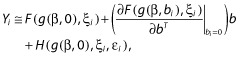
where y_ik, k = 1, …, K is the vector of n_ik observations for subject i and response k modelled as follows:

(5)

where f_k(.) is the structural model for the k^th response, θ_i is the i^th subject's parameter vector, h_k(.) is the residual error model for response k, often additive (h = ε_ik), proportional (h = f_k(·)ε_ik) or a combination of both, and ε_ik is the residual error vector for response k in subject i.

In this paper, additive (homoscedastic) or proportional (heteroscedastic) error models will be used in the examples so that only one residual variance parameter is defined for each response. To simplify notation, we assume that ε_ik are normally distributed and independent between responses (which is not necessary; see, e.g. [26,27]) with mean zero and variance . The individual parameter vector θ_i, with parameter(s) that might be shared between responses, is described as follows:

(6)

where β is the u-vector of fixed effects parameters, or typical subject parameter and b_i, the vector of the v random effects for the subject i defining the subject deviation from the typical value of the parameter. We assume that b_i is normally distributed with a mean of zero and a covariance matrix Ω of size v × v. Again, to simplify notation we assume a diagonal (which is not necessary; see, e.g. [18,27–29]) interindividual covariance matrix (Ω) with diagonal elements . The vector of population parameters is thus defined as follows:

(7)

where 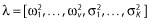is the vector of all variance components.

The population Fisher information matrix FIM(Ψ, Ξ) for multiple response models with the population design Ξ is given by:

(8)

where L(Ψ, Y) is the log-likelihood of all the observations Y given the population parameters Ψ.

Assuming independence across subjects, the log-likelihood can be defined as the sum of the individual contribution to the log-likelihood: 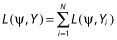. Therefore, the population Fisher information matrix (calculated using the second derivative of the log-likelihood) for N subjects can also be defined as the sum of the N elementary information matrices FIM(Ψ, ξ_i) computed for each subject i:

(9)

In the case of a limited number of L groups (where each individual in a group shares the same design), as in Equation (3), the population FIM is expressed by:

(10)

For one subject, given the design variables ξ_i and the NLMEM model, the FIM is a block matrix defined as:

(11)

where is the block of the Fisher matrix for the fixed effects β and is the block of the Fisher matrix for the variance components λ.

When a standard FO approximation of the model is performed (see Appendix), then the distribution of the observations in patient i with design ξ_i is approximated by Y_i ∼ N(E_i, V_i). Expressions for the population mean E_i and population variance V_i are given in the Appendix. The following expression for blocks A, B and C are obtained [18,30,31], ignoring indices i for simplicity:

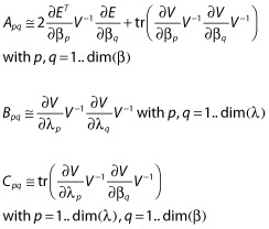(12)

This expression of the FIM [Equation (12)] will be referred to as the full FIM in this paper.

If the approximated variance V is assumed to be independent of the typical population parameters β, the matrix C will be zero and the matrices A and B will instead be defined as follows:

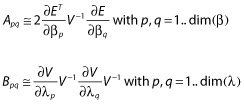(13)

which will be termed the block diagonal FIM in the following. The explicit formula for FIM(β, ξ_i) using the block diagonal form is given in the Appendix. More information about the derivation of the FIM or other approximations is reported in [27,28,30,32–34].

Software description

There are presently five software tools that implement experimental design evaluation and optimization of the FIM for multiple response population models. The five software tools are (in alphabetical order) PFIM [35], PkStaMp [24], PopDes [23], PopED [27,31] and POPT [21]. Four of them have been developed by academic teams.

PFIM (Population Fisher Information Matrix) is the only tool that uses the software R; the other software packages have been developed under the numerical computing environment MATLAB. The first version of PFIM appeared in 2001, and since this date several releases have been issued. It is available at http://www.pfim.biostat.fr. A graphical user interface (GUI) package using the R software (PFIM Interface) is also available but does not include recent methodological developments.

PkStaMp (Pharmacokinetic Sampling Times Allocation – Matlab Platform) is a library compiled as a single executable file, which does not require a MATLAB license. The developers can share the stand-alone version with anyone interested.

PopDes (Population Design) has been developed at the University of Manchester, and this application software has been available at http://www.capkr.man.ac.uk/home since 2007.

PopED (Population optimal Experimental Design), freely available at http://www.poped.sf.net, consists of two parts, a script version, responsible for all optimal design calculations, and a GUI. The script version can use either MATLAB or Freemat (http://www.freemat.sf.net; a free alternative to MATLAB) as an underlying engine. Some advanced PopED features, such as automatic and symbolic differentiation, Laplace approximation of Bayesian criteria and mode base linearization, are not available in FreeMat; however, all features presented in Table 1 are available in PopED using either FreeMat or Matlab.

Table 1.

Available features in the software tools available for population design evaluation

Feature	Software
	PFIM	PkStaMp	PopDes	PopED	POPT
Language	R	Matlab	Matlab	Matlab FreeMat	Matlab FreeMat
Available on website	✓		✓	✓	✓
Library of PKPD models	✓	✓	✓	✓	✓
User-defined models	✓	✓	✓	✓	✓
Multiresponse models	✓	✓	✓	✓	✓
Designs differ across responses	✓	✓	✓	✓	✓
ODE models	✓	✓	✓	✓	✓
Full FIM	✓	✓	✓	✓	–
Full covariance matrix for Ω	–	✓	✓	✓	–
Full covariance matrix for Σ	–	–	✓	✓	–
IOV	✓	–	✓	✓	–
Discrete covariates/power	✓/✓	–	✓/–	✓/✓	✓/–

Abbreviations are as follows: FIM, Fisher information matrix; GUI, graphical user interface; IOV, interoccasion variability; ODE, ordinary differential equation; PKPD, pharmacokinetic–pharmacodynamic; Σ, residual covariance matrix; Ω, interindividual covariance matrix.

POPT (Population OPTimal design) was developed from PFIM (MATLAB) in 2001 and is constructed as a set of MATLAB scripts. POPT requires MATLAB and can run on FreeMat. This tool can be downloaded on the website http://www.winpopt.com. All the software tools run on any common operating system platform (e.g. Windows, Linux, Mac).

Comparison of software for design evaluation

As we focus on design evaluation and not design optimization, we first compared the software tools with respect to: (i) required programming language; (ii) availability; (iii) library of PK and PD models; as well as ability to deal with: (iv) multiple response models; (v) models defined by differential equations; (vi) unbalanced multiple response designs; (vii) correlations between random effects and/or residuals; (viii) models including interoccasion variability (IOV); (ix) models including fixed effects for the influence of discrete covariates on the parameters; and (x) computation of the predicted power. Table 1 is a summary of the comparison of the software with respect to these different aspects. Globally, for all software tools, the library of PK models includes one-, two- and three-compartment models, with bolus, infusion and first-order (e.g. oral) administration, after a single dose, multiple doses and at steady state. Pharmacokinetics models with first-order elimination and models with Michaelis–Menten elimination are available. Regarding PD models, immediate linear and maximal effect (E_max) models and turnover response models are available.

Over recent years, those tools have included various improvements in terms of model specification and calculations of the FIM. For all of them, design evaluation can be performed for single or multiple response models either using libraries of standard PK and PD models or using a user-defined model. For the latter, regardless of the software used, the model can be written using an analytical form or using a differential equation system. In the case of multiple response models, population designs can be different across the responses for all the software. Regarding the calculations of the information matrix, the majority of the software can handle either a block diagonal Fisher information matrix (block FIM) or the full matrix (full FIM). Otherwise, only PopDes and PopED allow for calculations for a model with both correlation between random effects (full covariance matrix Ω) and correlation between residuals (full covariance matrix Σ); PkStaMp allows full covariance matrix Ω. It is possible in PFIM, PopDes and PopED to use models with IOV and models including fixed effects for the influence of discrete covariates on the parameters. The computation of the predicted power of the Wald test [30,36] for a given distribution of a discrete covariate can be evaluated in PFIM, PopDES and PopED frameworks.

Examples

Two different examples were used to illustrate the performance of the five population design software tools. Note that the examples evaluated the prediction for a given design, by evaluating the FIM and the predicted asymptotic SEs, without design optimization. This was done to evaluate the core calculations of the FIM. The FIM is evaluated with the full and the block diagonal derivation [Equations (12), (13)] with the different software tools.

In the first example, a one-compartment PK model (based on a warfarin PK model) with first-order absorption was used [35]. The design of that study consisted of 32 subjects with a single dose of 70 mg (a dose of 1 mg kg⁻¹ and a weight of 70 kg), and with eight sampling times postdose (in hours), as follows:

The residual error model was proportional (h = f·ε) with a coefficient of variation of 10% (σ² = 0.01), and exponential random effects were assumed for all parameters . Table 2 reports the model parameters and their values. The dose and design are based on [34,37].

Table 2.

Model parameters of warfarin pharmacokinetics model

Parameter	Value
βCL/F (l h−1)	0.15
βV/F (l)	8.00
βka (l h−1)	1.00
	0.07
	0.02
	0.60
σ2	0.01

Abbreviations are as follows: CL/F, apparent clearance of the warfarin; ka, constant of absorption of the warfarin; V/F, apparent volume of distribution of the warfarin; β, fixed effects; σ², residual variance; ω², interindividual variance.

For the second example, a multiple response PKPD model with repeated dosing was selected with the same design across responses [38]. The model describes hepatitis C virus (HCV) kinetics or, more specifically, the effect of a pegylated interferon dose of 180 μg week⁻¹ administered as a 24 h infusion once a week for 4 weeks. The same sequence of 12 sampling times for both PK and PD measurements (in days, post first dose) was used for 30 subjects:

The HCV model is described by the following system of ODEs:

where C(t) = A(t)/V_d is the drug concentration at time t and r(t) is the constant infusion rate. The viral dynamics model considers target cells (T), productively infected cells (I) and viral particles (W). Target cells are produced at a rate s and die at a rate d. Cells become infected with de novo infection rate e. After infection, these cells are lost with rate δ. In the absence of treatment, virus is produced by infected cells at a rate p and cleared at a rate c (for more details see [38,39]). The model for each response in subject i is defined as follows:

An additive error model was assumed for both PK and PD (log viral load) compartments, from which observations were drawn with a standard deviation of 0.2. Some of the parameters in the model are fixed (p, d, e and s). For the other seven parameters (k_a, k_e, V_d, EC₅₀, n, δ and c), log transformation was made with additive random effects on the log fixed effect with a variance (ω²) of 0.25. All parameters and their values are listed in Table 3.

Table 3.

Model parameters for hepatitis C virus pharmacokinetic–pharmacodynamic model

Parameter	Value
p (fixed)*	100
d (day−1) (fixed)*	0.001
e (ml day−1) (fixed) *	1E-07
s (ml−1 day−1) (fixed)*	20 000
βka (day−1)	0.80
βke (day−1)	0.15
βVd (ml)	100 000
(μg ml−1)	0.00012
βn	2
βδ (day−1)	0.20
βc (day−1)	7
	0.25
	0.25
	0.25
	0.25
	0.25
	0.25
	0.25
	0.04
	0.04

Abbreviations are as follows: c, rate constant of elimination of viral particles; EC₅₀, drug concentration in the blood at which the drug is 50% effective; ka, rate constant of absorption; ke, rate constant of elimination; n, Hill coefficient; Vd, volume of distribution; β, fixed effects; δ, rate constant of elimination of infected cells; , residual variance for the pharmacodynamic response; , residual variance for the pharmacokinetic response; ω², interindividual variance.

^*Parameters are defined in Examples section.

Methods

For each example using each software tool, we computed the FIM based on the FO linearization, given the parameters and the design. We used both the block diagonal and the full FIM (not available in POPT). From the FIM, we computed the predicted SE values for each parameter and the information D-criterion, which is defined as the determinant of the FIM to the power of one over the number of parameters: |FIM|^1/dim(Ψ).

To investigate the FIM predictive performance, the empirical SE values were also estimated using CTS. More precisely, for each example, multiple data sets were simulated and then fitted using the Stochastic Approximation Expectation Maximization (SAEM) algorithm in MONOLIX 2.4 (http://www.lixoft.eu) and, for the PK example, also with the FOCEI algorithm in NONMEM 7 (http://www.iconplc.com/technology/products/nonmem/). Empirical standard errors were derived from the estimated parameters. The empirical D-criterion was computed from the normalized empirical variance–covariance matrix of all estimated parameters, . Given that the CTS was much more time consuming for the HCV PKPD model, we did not perform the estimation with NONMEM and we carried out only 500 replicates, whereas we simulated 1000 replicates for the warfarin PK model.

For the CTS, to compute the empirical covariance matrix, the full variance–covariance matrix of all the estimated vectors was computed, not as two separate blocks for fixed effects and random components.

Results

For the PK model, the results show no differences between the optimal design software tools when evaluating the FIM using the block diagonal and full form. In the same way, all software reported the same expected D-criterion (Figure 1) and the same expected relative standard error (RSE) values expressed as percentages (Table 4).

Figure 1.

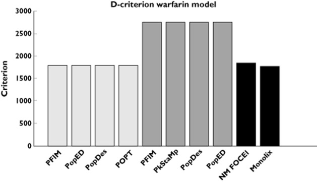
D-criterion predicted by the different software tools for the warfarin phamacokinetics model compared with simulated D-criterion calculated from the inverse of the empirical covariance matrix. NONMEM first-order conditional estimation method with interaction (NM FOCEI) is calculated from the estimates using the first-order conditional estimation method with interaction in NONMEM. The Monolix criterion is calculated from the estimates using the SAEM algorithm in Monolix. () block diagonal, () full and () simulated

Table 4.

Fisher information matrix (FIM) predicted relative standard errors (RSEs) (%) for warfarin pharmacokinetics model with the various software tools compared with empirical RSEs (%)

Parameter	Block diagonal FIM	Full FIM	Simulations
	PFIM/PkStaMp/PopDes/PopED/POPT	PFIM/PkStaMp/PopDes/PopED	NONMEM	MONOLIX
βka	13.9	4.8	13.6	13.8
βCL/F	4.7	3.6	4.9	4.8
βV/F	2.8	2.6	2.7	2.8
	25.8	26.5	26.6	28.1
	25.6	26.3	26.1	26.6
	30.3	30.9	32.4	30.8
σ2	11.2	12.4	10.9	11.0

Abbreviations are as follows: CL/F, apparent clearance of the warfarin; ka, constant of absorption of the warfarin; V/F, apparent volume of the warfarin; β, fixed effects; σ², residual variance; ω², interindividual variance.

In this example, the block diagonal FIM calculations gave an expected D-criterion that was very similar to the observed D-criterion based on the inverse of the empirical covariance matrix (Figure 1). However, for all software, the block diagonal D-criterion is slightly smaller than the NONMEM FOCEI-based criterion. Note that the result from MONOLIX is lower than the expected D-criteria, in line with theoretical expectations from the Cramér–Rao inequality (FIM is an asymptotic upper bound on the information). The full FIM predicts considerably more information compared with the simulations (expected D-criteria are larger than the observed values), and predicts total information that is further from the empirical values than the block diagonal calculations. The same trends are evident when looking at the RSE values, reported in Table 4. Good agreement between the CTS and the block diagonal FIM was found, while the full FIM predicted considerably higher precision in β_ka and β_CL/F.

For the more complicated PKPD model, results are summarized In Figure 2 and Table 5, where RSEs (as percentages) are reported. The D-criterion reveals negligible differences between any of the software (Figure 2) and also almost no difference between predicted SE values (Table 5). In this example, as in the PK example, using the block diagonal FIM gave D-criterion predicted values that were very similar to the D-criterion based on the inverse of the empirical covariance matrix (Figure 2). The full FIM predicts considerably more information compared with the simulations (expected D-criteria larger than the observed values) and predicts total information (D-criterion) that is further from the empirical values than the block diagonal calculations. The same trends are evident when looking at SE values for each parameter (Table 5). We found good agreement between CTS and the block diagonal FIM, while the full FIM predicted higher precision in numerous parameters than observed.

Figure 2.

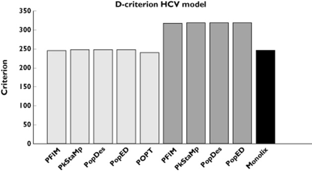
D-criterion predicted by the different software tools for the hepatitis C virus (HCV) model. Simulated D-criterion calculated from the inverse of the empirical covariance matrix. The Monolix criterion is calculated from the estimates using the SAEM algorithm in Monolix. () block diagonal, () full and () simulated

Table 5.

Fisher information matrix (FIM) predicted relative standard errors (RSEs) (%) for the hepatitis C virus model parameters with the various software tools compared with empirical RSEs

		Block diagonal FIM			Full FIM	Simulations
Parameter	PFIM	PkStaMp/PopDes/PopED	POPT	PFIM	PkStaMp/PopDes/PopED	MONOLIX
βka	12.0	12.1	13.2	8.6	8.6	12.2
βke	10.4	10.5	11.1	6.8	6.9	10.4
βVd	9.9	10.0	11.2	8.3	8.4	9.9
	15.8	15.8	15.7	13.6	13.5	14.5
βn	10.5	10.4	10.4	7.4	7.5	10.6
βδ	9.5	9.4	9.4	8.7	8.5	10.1
βc	11.1	11.0	11.0	8.8	8.7	10.3
	39.6	40.0	42.0	42.8	43.2	41.6
	30.4	30.8	31.6	36.4	37.2	34.4
	28.4	28.8	31.6	32.8	33.2	30.4
	60.8	60.4	60.0	66.4	66.4	53.2
	28.8	28.8	28.8	32.8	32.8	31.6
	27.2	27.2	27.2	32.4	31.6	31.6
	32.8	32.8	32.4	34.0	33.6	30.0
	9.0	8.5	8.3	9.3	8.5	10.0
	8.0	9.0	9.0	8.5	9.3	9.0

Abbreviations are as follows: c, rate constant of elimination of viral particles; EC₅₀, drug concentration in the blood at which the drug is 50% effective; ka, rate constant of absorption; ke, rate constant of elimination; n, Hill coefficient; Vd, volume of distribution; β, fixed effects; δ, rate constant of elimination of infected cells; , residual variance for the pharmacodynamic response; , residual variance for the pharmacokinetic response; ω², interindividual variance

Discussion

The first statistical developments for the evaluation of the FIM for NLMEM to compare and evaluate population designs without simulation were performed in the late 1990s. Since then, five different software tools have been developed. We have compared these tools in terms of design evaluation. Optimization was not considered in the present work. It should be noted that most software is under active development, with regular addition of new features.

We compared the expression of the FIM computed by the five different optimal design software packages for two examples. The first example was a simple PK model, for which the algebraic solution could be written analytically. When using the same approximation, all optimal design software packages achieved the same D-efficiency criterion and predicted RSE values (as percentages). The second example was more complex, had two responses (both PK and PD measurements), and the model was written as a series of five differential equations. For this example, the D-criterion and RSE comparisons revealed negligible differences between software. The differences could potentially be explained by the use of different differential equation solvers, methods of implementing multiple response calculations, methods for computing numerical derivatives, tolerance levels for ODEs and numerical implementations of matrix inverses and solving of linear systems, etc. These small differences could be seen even across the MATLAB computations of the FIM. In this work, we did not impose the same implementation of the various steps across software; hence, the importance of the present comparison.

In both examples, the expected SE values from the block diagonal FIM were close to the empirical SE values obtained from CTS. The runtimes for all software tools were a few seconds compared with minutes (warfarin example) or days (HCV example) for the CTS evaluation. Although computational speed has increased dramatically since the 1990s, a significant speed advantage is seen with the developed software tools even without considering design optimization. For instance, for the HCV PKPD model the CTS took several days for one design, so that optimization of doses and sampling times would be difficult.

In both examples investigated, the block diagonal FIM calculations give an expected D-criterion that is very similar to the observed D-criterion based on the inverse of the empirical covariance matrix, and RSE (%) values for parameter match well. In contrast, the full FIM predicts more information compared with the simulations (expected D-criteria larger than the observed values). More discussion on the assumptions beyond the block or full matrix can be found in [33], together with suggestions of other stochastic approaches. It seems that when using an FO approximation for computation of the FIM, linearization around some fixed values for the fixed effects, which are then no longer considered as estimable parameters and therefore correspond to the block diagonal matrix, provides the best approach. Also, higher order approximations to the FIM are available that may give better prediction of RSE (%) values [27].

Results using the simple FO approximation and the block diagonal FIM are very close to those obtained by CTS using both FOCEI and SAEM estimation methods in the two examples. However, as the expected FIM calculation is computing an asymptotically lower bound of the covariance of the parameters, and the calculations are based on approximations, we suggest that a CTS study of the proposed final design should be performed in order to evaluate the likely performance of the design in the setting in which it is proposed to be used. Given that this would be a single CTS at a specified design, this should not be computationally onerous compared with attempting to ‘optimize’ designs using CTS. In addition, using a CTS study of the final design makes it possible to assess the bias, which is not evaluated by the FIM.

In this first comparison between the software, we carried out only design evaluation for continuous data and using the simpler FO approximation of the FIM. This first step was necessary before the next work, where we will compare results of design optimization. Indeed, now that we know that similar criteria across software are obtained, we can compare the rather different optimization algorithms implemented. In principle, any design variable that is present in the model can be optimized within an optimal design framework. Examples of design variables that can be optimized are measurement sampling times, doses, distribution of subjects between elementary designs, number of measurement samples in an elementary design, etc. How this is done and which design variables can be optimized varies between software, but the independent variable (e.g. measurement sampling times) and the group assignment can be optimized in all software presented in this paper. Results will depend on the assumptions about the model and the parameter values, so that sensitivity studies should be performed to implement ‘robust’ designs, i.e. designs that are robust to the assumed a priori values of the parameters. Approaches for design optimization using a priori distribution of the parameters were suggested and implemented for standard nonlinear regression and extended to population approaches and should also be compared in further studies.

In conclusion, optimal design software tools allow for direct evaluation of population PKPD designs and are now widely used in industry [25]. Choice of software can depend on what platform the user has available and what features they are looking for, because the FIM calculation in the different software gives similar results. Population approaches are increasingly used for more complex/physiological PD models. It is very difficult to guess, without using one of these tools, what the good designs for those complex ODE models are and whether the study will be reliable. We suggest that before performing any population PKPD study, the design should be evaluated with a good balance between the approach based on the Fisher information matrix (for optimizing the design) and CTS (for evaluating the final design).

Appendix

Development of the FIM in NLMEM for multiple responses using FO approximation

For each subject i with design ξ_i, the elementary Fisher information matrix is defined as follows:

(14)

where L_i(Ψ, Y_i) is the log-likelihood of the vector of observations Y_i given the population parameters Ψ.

Let F(θ_i, ξ_i) = F(g(β, b_i), ξ_i) and H(θ_i, ξ_i, ε_i) = H(g(β, b_i), ξ_i, ε_i) be the vector composed of the K vectors of n_ik predicted responses f_k(θ_i, ξ_ik) and error h_k(θ_i, ξ_ik, ε_ik), respectively. Then Equation (5) can be written as follows:

(15)

As there is no analytical expression for the log-likelihood L_i(Ψ; Y_i) for nonlinear models, a first-order Taylor expansion around the expectation of b_i is used:

(16)

Then Equation (16) can be approximated as:

(17)

Therefore, Y_i ∼ N(E_i, V_i) approximately, with marginal expectation E_i and variance V_i given by:

(18)

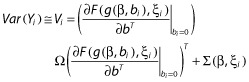(19)

where Σ(β, ξ_i) is the variance of H(g(β, 0), ξ_i, ε_i). Σ(β, ξ_i) has a simple expression for usual error models where ε_i enters linearly; otherwise, it can be computed using a first-order linearization of H around the expectation of ε_i.

Then the elementary FIM for the fixed effects using the block diagonal form [Equation (13)], has the following expression:

(20)

where

Of note, when Ω = 0, FIM(β, ξ_i) reduces to the FIM for individual nonlinear regression with parameters β.

Competing Interests

There are no competing interests to declare.

References

- 1.Box GEP, Lucas HL. Design of experiments in non-linear situations. Biometrika. 1959;46:77–90. [Google Scholar]
- 2.Draper NR, Hunter WG. The use of prior distributions in the design of experiments for parameter estimation in non-linear situations: multiresponse case. Biometrika. 1967;54:662–665. Epub 1967/12/01. [PubMed] [Google Scholar]
- 3.Atkinson AC, Hunter WG. The design of experiments for parameter estimation. Technometrics. 1968;10:271–289. [Google Scholar]
- 4.D'Argenio DZ. Optimal sampling times for pharmacokinetic experiments. J Pharmacokinet Biopharm. 1981;9:739–756. doi: 10.1007/BF01070904. [DOI] [PubMed] [Google Scholar]
- 5.Atkinson AC, Donev AN. Optimum Experimental Designs. Oxford: Clarendon Press; 1992. [Google Scholar]
- 6.D'Argenio DZ. Advanced Methods of Pharmacokinetic and Pharmacodynamic Systems Analysis. New York: Plenum Press; 1991. [Google Scholar]
- 7.Fedorov VV, Leonov SL. Optimal Design for Nonlinear Response Models. Boca Raton, FL: Chapman & Hall/CRC Biostatistics Series; 2013. [Google Scholar]
- 8.Landaw EM. Optimal Design for Individual Parameter Estimation in Pharmacokinetics. New York: Raven Press; 1985. pp. 181–8. [Google Scholar]
- 9.Pronzato L, Walter E. Robust experimental design via maximin optimization. Math Biosci. 1988;89:161–176. [Google Scholar]
- 10.Hennig S, Nyberg J, Fanta S, Backman JT, Hoppu K, Hooker AC, Karlsson MO. Application of the optimal design approach to improve a pretransplant drug dose finding design for ciclosporin. J Clin Pharmacol. 2012;52:347–360. doi: 10.1177/0091270010397731. Epub 2011/05/06. [DOI] [PubMed] [Google Scholar]
- 11.Merle Y, Mentre F, Mallet A, Aurengo AH. Designing an optimal experiment for Bayesian estimation: application to the kinetics of iodine thyroid uptake. Stat Med. 1994;13:185–196. doi: 10.1002/sim.4780130209. Epub 1994/01/30. [DOI] [PubMed] [Google Scholar]
- 12.Sheiner LB, Beal SL. Evaluation of methods for estimating population pharmacokinetic parameters. III. Monoexponential model: routine clinical pharmacokinetic data. J Pharmacokinet Biopharm. 1983;11:303–319. doi: 10.1007/BF01061870. Epub 1983/06/01. [DOI] [PubMed] [Google Scholar]
- 13.Al-Banna MK, Kelman AW, Whiting B. Experimental design and efficient parameter estimation in population pharmacokinetics. J Pharmacokinet Biopharm. 1990;18:347–360. doi: 10.1007/BF01062273. [DOI] [PubMed] [Google Scholar]
- 14.Ette EI, Kelman AW, Howie CA, Whiting B. Analysis of animal pharmacokinetic data: performance of the one point per animal design. J Pharmacokinet Biopharm. 1995;23:551–566. doi: 10.1007/BF02353461. Epub 1995/12/01. [DOI] [PubMed] [Google Scholar]
- 15.Jonsson EN, Wade JR, Karlsson MO. Comparison of some practical sampling strategies for population pharmacokinetic studies. J Pharmacokinet Biopharm. 1996;24:245–263. doi: 10.1007/BF02353491. [DOI] [PubMed] [Google Scholar]
- 16.Ette EI, Sun H, Ludden TM. Balanced designs in longitudinal population pharmacokinetic studies. J Clin Pharmacol. 1998;38:417–423. doi: 10.1002/j.1552-4604.1998.tb04446.x. Epub 1998/05/29. [DOI] [PubMed] [Google Scholar]
- 17.U.S. Department of Health and Human Services FaDA. 1999. Guidance for industry. Population Pharmacokinetics. [DOI] [PubMed]
- 18.Mentré F, Mallet A, Baccar D. Optimal design in random effect regression models. Biometrika. 1997;84:429–442. [Google Scholar]
- 19.Titterington DM, Cox DR. Biometrika: One Hundred Years. Oxford: Oxford University Press; 2001. [Google Scholar]
- 20.Retout S, Duffull S, Mentre F. Development and implementation of the population Fisher information matrix for the evaluation of population pharmacokinetic designs. Comput Methods Programs Biomed. 2001;65:141–151. doi: 10.1016/s0169-2607(00)00117-6. [DOI] [PubMed] [Google Scholar]
- 21.Duffull S, Waterhouse T, Eccleston J. Some considerations on the design of population pharmacokinetic studies. J Pharmacokinet Pharmacodyn. 2005;32:441–457. doi: 10.1007/s10928-005-0034-2. Epub 2005/11/15. [DOI] [PubMed] [Google Scholar]
- 22.Foracchia M, Hooker A, Vicini P, Ruggeri A. POPED, a software for optimal experiment design in population kinetics. Comput Meth Prog Bio. 2004;74:29–46. doi: 10.1016/S0169-2607(03)00073-7. [DOI] [PubMed] [Google Scholar]
- 23.Gueorguieva I, Ogungbenro K, Graham G, Glatt S, Aarons L. A program for individual and population optimal design for univariate and multivariate response pharmacokinetic-pharmacodynamic models. Comput Methods Programs Biomed. 2007;86:51–61. doi: 10.1016/j.cmpb.2007.01.004. [DOI] [PubMed] [Google Scholar]
- 24.Aliev A, Fedorov V, Leonov S, McHugh B, Magee M. PkStaMp Library for constructing optimal population designs for PK/PD Studies. Commun Stat Simul Comput. 2012;41:717–729. [Google Scholar]
- 25.Mentré F, Chenel M, Comets E, Grevel J, Hooker A, Karlsson MO, Lavielle M, Gueorguieva I. 2012. Current use and developments needed for optimal design in pharmacometrics: a study performed amongst DDMoRe's EFPIA members. [DOI] [PMC free article] [PubMed]
- 26.Gueorguieva I, Aarons L, Ogungbenro K, Jorga KM, Rodgers T, Rowland M. Optimal design for multivariate response pharmacokinetic models. J Pharmacokinet Pharmacodyn. 2006;33:97–124. doi: 10.1007/s10928-006-9009-1. Epub 2006/03/22. [DOI] [PubMed] [Google Scholar]
- 27.Nyberg J, Ueckert S, Stromberg EA, Hennig S, Karlsson MO, Hooker AC. PopED: an extended, parallelized, nonlinear mixed effects models optimal design tool. Comput Methods Programs Biomed. 2012;108:789–805. doi: 10.1016/j.cmpb.2012.05.005. Epub 2012/05/30. [DOI] [PubMed] [Google Scholar]
- 28.Gagnon R, Leonov S. Optimal population designs for PK models with serial sampling. J Biopharm Stat. 2005;15:143–163. doi: 10.1081/bip-200040853. Epub 2005/02/11. [DOI] [PubMed] [Google Scholar]
- 29.Ogungbenro K, Graham G, Gueorguieva I, Aarons L. Incorporating correlation in interindividual variability for the optimal design of multiresponse pharmacokinetic experiments. J Biopharm Stat. 2008;18:342–358. doi: 10.1080/10543400701697208. Epub 2008/03/11. [DOI] [PubMed] [Google Scholar]
- 30.Retout S, Mentré F. Further developments of the Fisher information matrix in nonlinear mixed effects models with evaluation in population pharmacokinetics. J Biopharm Stat. 2003;13:209–227. doi: 10.1081/BIP-120019267. [DOI] [PubMed] [Google Scholar]
- 31.Foracchia M, Hooker A, Vicini P, Ruggeri A. POPED, a software for optimal experiment design in population kinetics. Comput Methods Programs Biomed. 2004;74:29–46. doi: 10.1016/S0169-2607(03)00073-7. [DOI] [PubMed] [Google Scholar]
- 32.Leonov S, Aliev A. Optimal design for population PK/PD models. Tatra Mt Math Publ. 2012;51:115–130. [Google Scholar]
- 33.Mielke T, Schwabe S. Some considerations on the Fisher information in nonlinear mixed effects models. In: Giovagnoli A, Atkinson AC, Torsney B, editors. mODa 9 – Advances in Model-Oriented Design and Analysis. Berlin: Physica-Verlag/Springer; 2010. pp. 129–136. [Google Scholar]
- 34.O'Reilly RA, Aggeler PM, Leong LS. Studies on the coumarin anticoagulant drugs: the pharmacodynamics of warfarin in man. J Clin Invest. 1963;42:1542–1551. doi: 10.1172/JCI104839. Epub 1963/10/01. [DOI] [PMC free article] [PubMed] [Google Scholar]
- 35.Bazzoli C, Retout S, Mentre F. Design evaluation and optimisation in multiple response nonlinear mixed effect models: PFIM 3.0. Comput Methods Programs Biomed. 2010;98:55–65. doi: 10.1016/j.cmpb.2009.09.012. Epub 2009/11/07. [DOI] [PubMed] [Google Scholar]
- 36.Retout S, Comets E, Samson A, Mentre F. Design in nonlinear mixed effects models: optimization using the Fedorov-Wynn algorithm and power of the Wald test for binary covariates. Stat Med. 2007;26:5162–5179. doi: 10.1002/sim.2910. Epub 2007/05/09. [DOI] [PubMed] [Google Scholar]
- 37.O'Reilly RA, Aggeler PM. Studies on coumarin anticoagulant drugs. Initiation of warfarin therapy without a loading dose. Circulation. 1968;38:169–177. doi: 10.1161/01.cir.38.1.169. Epub 1968/07/01. [DOI] [PubMed] [Google Scholar]
- 38.Guedj J, Bazzoli C, Neumann AU, Mentre F. Design evaluation and optimization for models of hepatitis C viral dynamics. Stat Med. 2011;30:1045–1056. doi: 10.1002/sim.4191. Epub 2011/02/22. [DOI] [PubMed] [Google Scholar]
- 39.Neumann AU, Lam NP, Dahari H, Gretch DR, Wiley TE, Layden TJ, Perelson AS. Hepatitis C viral dynamics in vivo and the antiviral efficacy of interferon-alpha therapy. Science (New York, NY) 1998;282:103–107. doi: 10.1126/science.282.5386.103. Epub 1998/10/02. [DOI] [PubMed] [Google Scholar]