Covariate selection in pharmacometric analyses: a review of methods

Abstract

Covariate selection is an activity routinely performed during pharmacometric analysis. Many are familiar with the stepwise procedures, but perhaps not as many are familiar with some of the issues associated with such methods. Recently, attention has focused on selection procedures that do not suffer from these issues and maintain good predictive properties. In this review, we endeavour to put the main variable selection procedures into a framework that facilitates comparison. We highlight some issues that are unique to pharmacometric analyses and provide some thoughts and strategies for pharmacometricians to consider when planning future analyses.

Introduction

Pursuit and identification of the ‘best’ regression model has a long, rich history in the sciences. Data analysts had several motivating factors when searching for a model to describe their data. Designing, conducting and analysing an experiment could be a lengthy and costly process. Finding the key predictors of the response could reduce the cost by eliminating extraneous conditions that did not need to be studied in the next experiment. Such a reduction in the dimensionality of the problem appealed not only to the intellectual principle of parsimony (a heuristic stating that simpler, plausible models are preferable), but had practical appeal; simpler systems were easier to understand, discuss and implement. This resonated with data analysts, especially prior to the age of high-speed computers. Much of the early 1960s literature on variable selection was devoted to organizational methods for efficient variable selection by desktop calculator or even by hand [1–3]. Some of these considerations are still applicable to pharmacometric analyses in the present age even though some contexts may have changed subtly.

The focus of this review is on methods for the selection of covariates or predictors, i.e. patient variables, either intrinsic or extrinsic, that attempt to explain between-subject variability in the model parameters.1 For clarity, we make a distinction in this article between the effects of predictors (covariates) and parameters. Parameters are defined here to be quantities integral to the structure of the model and that usually have scientific interpretation in and of themselves, e.g. clearance (CL), volume of distribution (V), maximum effect (E_max) or concentration yielding half E_max (EC₅₀). The effects of predictors are defined as those which manifest the influence of a variable on one of the parameters. In pharmacometrics literature, the terms ‘covariate’ and ‘predictor’ are often used interchangeably, with ‘covariate’ being used more often. These terms can be used interchangeably throughout this article as well. Historically, however, these two terms are not identical in meaning. The term ‘covariate’ stems from analysis of covariance (ancova) and is defined more purely as a continuous variable used to control for its effect when testing categorical, independent variables, such as treatment levels. We also differentiate from those variables specified in the design that are more structural, which we denote here as independent variables, also to promote clarity. For example, one might consider dose and time to be independent variables in a pharmacokinetic (PK) model. Investigators may apply statistical hypothesis tests to independent variables, e.g. assessment of dose proportionality. However, such evaluations are usually performed when trying to determine a basic structural model (i.e. when defining the model parameters) and, as such, play a larger role when assessing goodness of fit (often using residuals), but are rarely associated with variable selection procedures. Predictor variables in clinical drug development are typically sampled randomly from the population, yet often have truncated distributions with specific ranges due to inclusion/exclusion criteria. For example, a clinical trial may be conducted in the elderly. The inclusion/exclusion criteria may set an age threshold, which defines what is considered elderly. However, the protocol is unlikely to set specific requirements for such numbers at each age when recruiting for the study. This also occurs in renal impairment studies. Subjects are stratified by certain categories of renal impairment, yet within each group the calculated creatinine clearance (CLcr) varies randomly. There is another consideration for pharmacometric analyses that is not typical for standard regression. In standard regression, each predictor usually is associated with one fixed effect or coefficient. This one-to-one relationship is not commonplace in pharmacometric analysis, where it is not atypical for each predictor variable to be associated with more than one parameter. A notable example is the allometric specification of bodyweight on CL and V in PK [4]. In this review, we use the term ‘predictor effects’ or ‘effects’, instead of just ‘predictors’ to maintain clarity that predictor variables can have more than one effect, hence more than one coefficient that needs to be estimated in the model. This distinction has a bearing on pharmacometric analysis and will be discussed in greater detail below.

We limit the scope of our review to methods specifically designed for selection of nested predictor effects, i.e. the determination that an effect is included or excluded from the parameter submodel. Exclusion occurs when the coefficient is fixed to the null effect value, which is typically zero for predictors incorporated in an additive fashion or one for those incorporated multiplicatively. The requirement that the effects be nested keeps with the classical distributions of the test statistics used in the procedures. We do not provide details on methods that do not allow for exclusion of a predictor effect. Methods such as ridge regression [5] and principal component regression [6,7] do not attempt specifically to identify effects for exclusion and are also not generally applicable to generalized nonlinear mixed-effects models (GNLMEMs) [8]. These methods do provide some interesting insight into issues associated with collinearity or correlation between predictor variables and will be discussed in this context only.

We also do not discuss general issues associated with model or submodel selection. An example of model selection is the process of identifying the number of compartments in a PK model (e.g. see [9]). Such models are typically not nested; for example, the one-compartment model space is not completely contained in the two-compartment model space. While not nested, the one-compartment model is a limiting case of the intercompartmental distribution rate constant going to zero or infinity and, as such, the log-likelihoods will share identical values when these parameters of the two-compartment model approach the boundary. Such evaluations require less standard (more technical) statistical considerations. Submodels are defined here as the functional form by which the predictor effect affects the parameter or enters into the model. Such specification is unique to nonlinear mixed-effects analysis and the desire to predict individual time–response profiles. We assume that the choice between submodels has been made prior to selection (inclusion or exclusion) of the effect. For example, we assume the choice between 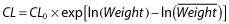, a typical power model, or 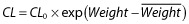for modelling clearance as a function of weight (Weight) has been made prior to evaluating whether weight is influential (CL₀ and 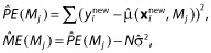are the reference clearance and weight, respectively). Such evaluations are also not nested, so the distributions of the test statistics for such comparisons are not standard. Bayesian model averaging [10] and the more recent frequentist model averaging [11], despite their potential value to pharmacometric analysis, are also not discussed. The methods are not specifically focused on reducing the dimensionality of the predictor effects and, as such, do not consider the value and interpretation of a predictor per se. Often, prediction and interpretation of a predictor variable are desirable because there is some intrinsic value in this knowledge (such as which predictors have enough ‘value’ that these should be included in a product label).

We are conscious that many readers are familiar, at least somewhat, with the popular stepwise variable selection procedures and even the issues associated with these. As a reviewer pointed out, our exposition is somewhat statistical. We have tried to provide clarification in the text and extended descriptions in an attempt to keep the reader from being bogged down by notation. We have attempted to use this notation to present these methods in a way that will allow comparisons with other procedures that are not as popular, yet are worth discussing.

The article is organized as follows. The next section discusses known issues with variable selection methods and strategies for mitigating some of the issues prior to undertaking such procedures. The following section discusses variable selection methods we feel are relevant to the past, present and near future of pharmacometric analyses. Many of the issues presented here that are interesting, in our opinion, are not about the variable selection methods per se; rather, issues that came from research, contemplation of the literature results and our own experiences, about focusing on strategies to mitigate known or anticipated issues germane to pharmacometric analyses.

Considerations prior to performing selection of predictor or covariate effects

We will assume the investigator has found an adequate and sufficient base structural and statistical model prior to performing the selection procedures. The term ‘base’ is used to indicate that no candidate predictor effects have yet been included in the model. Effects known to be predictive or influential can have been included; these are not intended to be evaluated by the selection procedure. For example, the investigator may wish to include the effect of creatinine clearance (CLcr) on CL in the base model for a compound known to be eliminated renally. We also assume the investigator has evaluated the goodness of fit with regard to standard likelihood assumptions, or the investigator has carried out due diligence in evaluating the adequacy of approximate models with regard to predictors on parameters of key interest [12]. Interactions between structural, statistical and predictor effects have been reported in the literature [13]. Such issues should be kept in mind, yet are not examined explicitly here. If such issues are thought to exist because of an inadequate design, simulation studies might be performed to help identify the key issues.

The development of computers gave investigators greater flexibility and ability to evaluate the effects of predictors. As such procedures were implemented more frequently, the focus shifted to understanding their properties. Several excellent review articles exist for ordinary least-squares (OLS) regression. Hocking [14] provides a thorough review and analysis of such. The issues identified in these reviews are worth consideration, and so we now discuss some of the technical results, theoretical and simulation-study based, that have shaped opinions on variable selection.

A key quantity used in OLS is the X′X matrix, where X is the matrix of predictor and/or independent variables. A fundamental result in OLS is 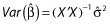, where is the vector of estimated coefficients, is the estimated residual variability, and Var(·) represents taking the variance. The equation effectively states that the standard errors of (the precisions in) the estimated coefficients depend upon the residual variability and also upon X. More specifically, the expected distance between the OLS estimate and the true coefficient β is related to the residual variance and the sum of the inverse of the eigenvalues of X′X. Thus, if X′X is unstable due to correlations between the predictors, some of the eigenvalues of X′X will be close to or equal to zero. As a result, , despite being unbiased, may yield predictions of poor quality because of the variability in the estimates. Consideration of X is thus important. One can see that if X′X has any zero eigenvalues, then the number of predictors in X should be reduced in some way by the number of zero eigenvalues. If some of the eigenvalues of X′X are small, a more likely occurrence in pharmacometric analyses, then it is unclear how to proceed. We term correlations between variables in X as a priori correlation, because it can be evaluated prior to any model fitting. We recommend computing the eigenvalues of the predictors (i.e. X′X matrix) even for pharmacometric analyses. We feel the eigenvalue approach to be better than pair-wise correlation plots for assessing correlations between the predictors because of the obvious issue with determining correlations between continuous and categorical covariates, and suggest that investigators routinely calculate and report these eigenvalues. One might prefer computing these eigenvalues after computing the ‘correlation matrix’ of X because the predictors will be unitless (and scaled).

If moderate or severe correlations between the variables in X exist, many suggest reducing or limiting the set to plausible predictors in X. Use of data-reduction techniques, such as using results in the literature to eliminate unlikely predictors, is considered good practice [15]. This is because the model has difficulty deciding on which predictor effects are influential when X′X is unstable. Derksen and Keselman [16] demonstrated that the magnitudes of the correlations between the predictor variables affected the selection of true predictor variables [16].

A considerable amount of influential work was done to overcome issues with the X′X matrix. Such works eventually inspired some newer and promising methods used today in variable selection (and are discussed below). Ridge regression is one such method developed to overcome the issue of an unstable X′X [5]. The method uses a tuning constant that governs the amount of augmentation to X′X, thereby stabilizing it, and was developed primarily for prediction, not variable selection. We note that there is an inherent suggestion by the method for deletion of variables, which results from the rapid convergence of some coefficient estimates to zero as the tuning constant is increased [17] (foreshadowing the newer methods). Kendall and Massy advocated transforming X′X to orthogonal predictors determined by the eigenvectors and deleting those with small eigenvalues [6,7]. The new matrix is constructed as linear combinations of the prior predictors. However, this does not reduce the dimensionality of the original predictors necessarily, in the sense that all of the original predictors could be combined into a single new predictor variable. Principal component regression has not been used in pharmacometric modelling, probably due to the difficulty in interpreting the coefficients and the derived predictors in a clinical context. The method does reduce the dimensionality with respect to prediction, but not with respect to interpretation of the original predictors which are meaningful. It is also unclear how one would deal with the same predictor in potentially different sets of predictors for each parameter, which is a salient issue in pharmacometric analyses.

It is easy to see that if the predictors in X are correlated, then pharmacometric models will have issues even though GNLMEMs do not use X′X explicitly during estimation. As stated above, we recommend computing the eigenvalues of X′X to assess the degree of correlation between the predictors. If the degree is high, then predictors should be removed from the set of candidates, preferably based on information not obtained from the data directly, but using preclinical findings or literature results from well-powered and well-analysed studies that found no effect of the predictor. A large condition number (the ratio of the largest to smallest eigenvalue from the correlation matrix of X′X) indicates that the predictors are highly correlated. Managing a priori correlation should help to reduce the number of spurious effects found in GNLMEM analyses.

There are some unique issues associated with GNLMEMs as implemented in pharmacometric analyses, to which we have alluded. Pharmacometric models are typically composed of key structural parameters. Submodels for evaluating predictors are constructed for each of the parameters of interest. Thus, the same predictor variable can be evaluated on more than one parameter (e.g. bodyweight on CL and V) and thus have more than one effect or coefficient for the predictor variable. Figure 1 provides examples of submodels for a PK and a pharmacokinetic–pharmacodynamic (PK-PD) model. Testing even a few predictors in multiple parameter submodels can lead to the estimation of a large number of coefficients due to the multiplicity.

Figure 1.

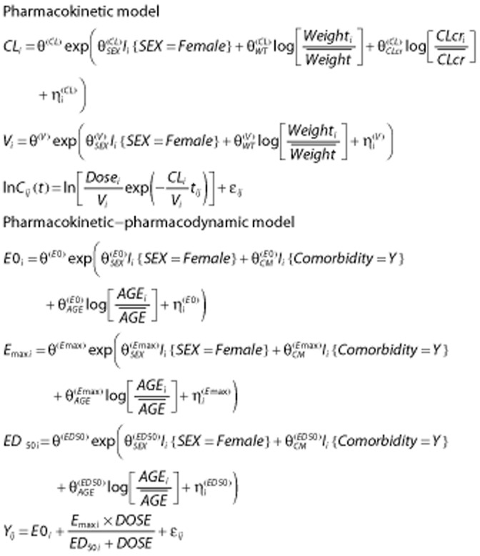
Examples of pharmacokinetic and pharmacokinetic–pharmacodynamic models. I{·} represents and indicator function that = 1 when the condition in braces is true and = 0 otherwise. A variable with bars represents some summary of the variable (e.g. median) for reference

Other issues can arise from correlations induced in the estimates because of an inadequate design. Even though one has identified a set of predictors that is a priori relatively uncorrelated, the design can induce a posteriori correlation. For example, consider a trial conducted with a dose range that spans from zero (placebo) to a level that achieves less than half the maximal drug effect (i.e. the ED₅₀). The estimates for the E_max and ED₅₀ parameters will be highly correlated. Such correlation can leak into the estimates of the effects. The information content in the data does not have sufficient resolution to determine whether the effects of predictors influence the E_max or the ED₅₀. Thus, in contrast to ordinary regression, spurious findings can result not only from selecting the wrong predictor, but also from selecting its effect on the wrong parameter. Confusion as to which parameter a predictor should be associated was found in an analysis performed by Hutmacher et al. [18]. In that case, the model had difficulty selecting between effects on hysteresis (time of onset of the effect) or potency, two parameters that have very different interpretations for how best to dose a subject long term.

Owing to the multiple effects of predictors and the potential interactions between design and parameters (and effects) in GNLMEM analyses, it is worth discussing the estimated covariance matrix of the maximum likelihood estimates (COV). In many ways, the COV is to GNLMEM what is to OLS regression. The COV is typically computed using the inverse Hessian matrix of the negative log-likelihood evaluated at the maximum likelihood estimates (MLEs), where the Hessian matrix is the matrix of second derivatives. Most GNLMEM software packages provide this as standard output. The Hessian is thus the observed (Fisher) information matrix. This is in contrast to the Fisher information matrix, which is calculated by taking the expected value (and is thus unconditional [19]). The information matrices, and hence COV, depend upon the model, the independent variables (i.e. the design) and predictor variables. A correlation matrix of the estimates can be computed from the COV matrix, and is also reported typically by software. We refer to this as a posteriori correlation. Correlation between the parameters and their predictors induced by either design and/or collinearity of the predictors can be assessed only from the COV or some other estimate thereof (such as a bootstrap [20]). Computing the eigenvalues of the correlation matrix is helpful for assessing the correlation. This is discussed more below.

We thus provide the following suggestions for consideration during the planning stages of variable (predictor) selection for pharmacometric applications of GNLMEM analyses. A list of parameters should be compiled, and the specific sets of predictor variables corresponding to these should be prepared prior to the analysis. Also, we do not recommend evaluating correlated covariates such as bodyweight and body mass index simultaneously in a selection procedure. Selection of one by scientific argument is preferable, if possible. Given that the number of predictors considered in X was found to be related to the number of spurious predictors selected by the procedure [16,21], only scientifically plausible predictors of clinical interest should be considered. For the PK example in Figure 1, the first table row would specify Sex, Weight and CLcr on CL and Sex and Weight on V. This should be done at the analysis planning stage, if preparing a plan, which we feel should be done for regulatory submission work. If there is no prior modelling experience with the drug, such that the parameters of the structural model are not known, then the predictors should be associated with concepts of parameters; for example, baseline, maximal drug effect, maximal placebo effect, placebo effect onset rate constant, drug effect onset rate constant, etc. One might not wish to test a predictor on all parameters; for example, not testing CLcr on V (as in Figure 1). Careful planning here when considering predictor–parameter relationships is wise because it will help to prevent spurious results that are difficult to explain or interpret, which can then lead to additional ad hoc (not prespecified) analyses of predictors that are hard to rationalize or defend. In our experience, such analyses are done quite often when a nonsensical predictor from a poorly defined analysis is selected (and not to the analyst's liking). An example is finding that CLcr affects the apparent absorption rate constant (k_a) and then rationalizing that this is because it is correlated with bodyweight.

Although this review considers such work to have been performed prior to variable selection, we specifically note that the issues and strategies discussed here are best detailed in an analysis plan formulated before any component of the data has been manipulated.

Variable selection criteria

According to Hocking, there are three key considerations for variable selection: (i) the computational technique used to provide the information for the analysis; (ii) the criterion used to analyse the variables and select a subset: and (iii) the estimation of the coefficients in the final equations [14]. Often, these three are performed simultaneously without clear identification. In the GNLMEM case, (i) will typically be differences in the −2 × log-likelihood (−2LL) values with a penalty (different from Hocking) between models. For (ii), some method (such as stepwise procedures) is chosen, often considering only computational expenditure. This is the focus of the next section. The third component is more subtle. Often (iii) is not considered by the analyst, but it can be important and is discussed in the Discussion section. Much of the traditional literature, as well as more recent pharmacometric literature, attempts to address the influence of the choice of (ii) on the results presented in (iii).

Likelihood-based methods are typically used in pharmacometric work, because maximum likelihood-based estimation is the primary method used and provides an objective function value at minimization (OFV) that either differs from the −2LL by a constant k (OFV = −2LL + k) or is equal to it (k = 0). Inclusion of the constant is immaterial. Consider a model M₁ with q₁ estimated coefficients, and a model nested within it, M₂ which has q₂ estimated coefficients. That is, M₂ can be derived from M₁ by setting some of its coefficients to the null value. The notation M₁ ⊃ M₂ represents the nesting and implies that M₁ is larger or richer than M₂, i.e. q₂ < q₁. The difference between the OFVs is ΔOFV(M₂, M₁) = OFV(M₂) − OFV(M₁), with ΔOFV(M₂, M₁) ≥ 0 because OFV(M₂) ≥ OFV(M₁). The nesting implies that the richer model must provide a ‘better’ fit (lower OFV) to the data at hand. The ΔOFV provides a statistic for the relative improvement in fitness for M₁ over M₂. The χ² distribution with q = q₁ – q₂ degrees of freedom (df) is a large sample approximation of the distribution of ΔOFV. When a P-value is calculated using ΔOFV for a prespecified two-sided hypothesis test of level α (i.e. type 1 error), the test is known as a likelihood ratio test (LRT) [22]. If P-value < α, the alternative hypothesis is accepted and M₁ is selected; if not, it is concluded that insufficient information is available to indicate that M₁ should be selected (note that one should not conclude the null hypothesis of no effect). The test as specified is formulated to evaluate whether the smaller model can be rejected in favour of accepting the larger model. It should be noted that when the likelihood is approximated using Laplace-based methods (including first-order conditional estimation or FOCE [23]), the OFV approximates −2LL + k and asymptotically approaches it in certain conditions [24].

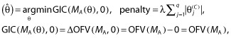
Variable selection in pharmacometrics work is primarily based on the LRT concept. This formulation is generalized here and intended to divest the remainder of the discussion from the LRT interpretation. To judge whether the improvement in fitness by the lower OFV for the fuller model is enough to justify the cost of estimating the coefficient of the effect, a penalty is applied to the ΔOFV statistic. The penalty is the cost in information required to include the effect, and it is used to avoid overfitting. This leads to what we will term a ‘general information criterion’ (GIC):

(1)

The larger dimensional model (M₂) is preferred when the GIC is > 0, and the smaller model (M₁) when the GIC is < 0. The most popular choices of the penalty are based on cut-off values, which are determined by selecting α levels from the χ² distribution; for example, the cut-off c is the value of the χ² cumulative distribution function for = 1 – α with df = q₁ – q₂. Typical α level choices with df = 1 are 0.05, 0.01 and 0.001, and these correspond to a c of 3.841, 6.635 and 10.828, respectively. The α levels in pharmacometrics are much smaller than those used in ordinary regression, for example; see Wiegand [1]. We surmise that the higher penalty values are chosen due to the legacy of the perception of poor performance of the LRT for the first-order (FO) estimation methods [23] and its inadequate approximation of the likelihood, or perhaps in an attempt to adjust for the multiplicity of testing. Wählby et al. confirmed this perception of the FO method, and also evaluated the type 1 error for the FOCE methods under various circumstances [25]. Beal provided a commentary which discussed, somewhat cryptically, the issues associated with significance and approximation of the likelihood [26]. It is important to note that even though a cut-off is based on an chosen α level, the variable selection procedure will not maintain the properties of an α level test, nor should selected effects be interpreted in such a light.

Other penalty values can be used for the GIC. The Akaike information criterion (AIC) [27] and Schwarz's Bayesian criterion (SBC), which is also known as the Bayesian information criterion (BIC), are notable. The AIC uses penalty = 2 × (q₂ – q₁), which corresponds interestingly to an α level = 0.157 when q₂ – q₁ = 1. A small sample correction for AIC was proposed by Hurvich and Tsai, but is beneficial at sample sizes (when the ratio of effects to data points is not large) smaller than typically found in clinical pharmacometric data sets [28]. The BIC uses penalty = (q₂ – q₁) × ln(n_E), where we refer to n_E as the effective sample size [29]. How to calculate n_E has been debated. In fact, SAS is inconsistent in this matter. PROC MIXED for linear mixed effects model uses the total number of evaluable data points (n_T), while PROC NLMIXED uses the number of subjects contributing data (n_S). It is clear that the n_S represents the sample size, which is completely independent (individuals represent independent pieces of information). Jones [30] states that longitudinal data are not completely independent and that n_T yields a penalty that is inappropriately high for GLNMEM, yet using n_S would be too conservative. The appropriate n_E is n_S < n_E < n_T, and he suggests a method for calculating n_E from the model fit.

Efforts have been made to compare the AIC and BIC. Clayton et al. state that the BIC in large samples applies a fixed and (nearly) equal penalty for choosing the wrong model and that this suggests that the AIC is not asymptotically optimal nor is it consistent (i.e. it does not select the correct model with probability one as the sample size increases) [31]. They do state that the AIC is asymptotically Bayes with penalties that depend upon the sample size and the kind of selection error made. Moreover, they state the AIC imposes a severe penalty when a ‘false’ lower dimensional model is selected as opposed to selecting a ‘false’ higher dimensional model, and that this could make good sense for prediction problems. The authors then evaluate these in the context of prediction error. Harrell Jr discusses these as well [15]. Overall, it is clear from the form of the penalties that the BIC will lead to selection of fewer predictor effects in general. While AIC and BIC are the most popular, other penalties have been derived. Laud and Ibrahim [32] note some of these.

Variable selection procedures

We loosely define the concept of the model space next, prior to discussion of the variable selection procedures. Conceptualization of the model space helps to illustrate the differences between the variable selection methods. Often, the model space is defined by the following. Let q be the number of candidate predictor effects being considered, derived from the unique presence or absence of each effect (i.e. q is the sum of the number of coefficients per parameter over the number of parameters). The support of the model space M is the set of all possible candidate models and thus has 2^q elements. However, we deviate from this formulation to provide more flexibility in evaluating models. The investigator may wish to evaluate some effects in groups. For example, the investigator may wish to lump all the coefficients for different race groups into one set of effects called RACE, rather than evaluate these by individual classifications (such as White, Black, etc). Therefore, we will consider evaluation of sets of predictor effects. The ‘each effect evaluated separately’ convention discussed above is a special case of our formulation. After forming these effect sets, let there be p of these (p ≤ q with equality only if there is one effect per set). Indexing the sets of effects from one to p, the base model with no sets of effects is defined as M₀ = {}, and the full model is M_A = {1, 2, …, p}, with all sets of effects in the model. Numbers in the brackets indicate the sets of effects included (coefficients estimated) in the model. Note that another convention for representing the model space is convenient when considering the genetic algorithm (discussed below). For this binary convention, each model is represented as a set with p elements, each of which can be zero for exclusion or one for inclusion of a set of effects. That is, M₀ = {0, …, 0}, M_A = {1, …, 1}, and M_gj = {0, …, 0, 1, 0, …, 0, 1, 0 … 0} is the model with the gth and jth sets of effects included (coefficients estimated).

The objective of the variable selection is to find the ‘best’ or optimal model according to some specified criteria. Most of the methods discussed here use the GIC values across the model space in an attempt to find the optimal model. Thus, the shape of the model space is defined by the GIC values, which are influenced by the following factors: (i) the observed response data; (ii) the independent predictor data (such as dose and time, i.e. the design); (iii) correlations between the predictor variables; (iv) correlations between the estimates of the structural parameters and coefficients, i.e. the a posteriori correlation; and (v) the choice of penalty applied by the investigator. The final model is based on the effects selected by the procedure.

Stepwise procedures

Stepwise procedures are the most commonly used in pharmacometric analyses. There are three basic types, namely forward selection (FS), backward elimination (BE) and classical stepwise. A fourth procedure is also used often; it is a combination of the FS and BE procedures.

The FS procedure begins with the base model, M₀. Let M_gj = {j, g}, which defines the model with the gth and jth set of effects included. In Step 1, models M₁, M₂, … M_p are fitted, and the GIC for each model M_i relative to M₀ is computed, i.e. GIC(M₀, M_i). The M_k with the largest GIC > 0 is selected for Step 2 (note that M₀ ⊂ M_k). If all GIC < 0, then the procedure terminates and M₀ is selected. In Step 2, models M_1k, M_2k, …, M_k−1k, M_{k k+1}, …, M_kp are fitted, the GIC(M_k, M_ik) values are computed, and the model M_kw with the largest GIC > 0 is selected for Step 3 (note that M₀ ⊂ M_k ⊂ M_kw; the model is becoming richer, and the indices are in numerical order, not the order of inclusion). This continues until all the GIC < 0 for a step. When this occurs, the reference model from the previous step is selected as the final. One can see why the penalty is often called the stopping rule in the literature.

This procedure is computationally economical. If the procedure completes the maximum possible p number of steps, only ½p(p + 1) models are fitted. However, it is also easy to see that this procedure ignores portions of the model space after each step based on the result of the step. The path through the model space is represented by M₀ ⊂ M_k ⊂ M_kw … M_ijkmw. Randomness in the data could lead to selecting a model at a step that precludes finding the best model. If, in the example, the path M₀ ⊂ M_k ⊂ M_ky was selected due to randomness, M_kw is no longer on the path, and thus, certain parts of the model space are no longer reachable. Ultimately, FS does not guarantee that the optimal model will be found, but it is computationally cheap, which can be an advantage for models with long run times. The FS procedure is illustrated in Figure 2a through an example. It is also noted that the order of effect selection does not confer the importance of the covariate predictor [33]. It has been observed that covariates selected for inclusion in an early step of the FS procedure may have less predictive value once other covariate parameters are included in subsequent steps.

Figure 2.

An illustration of two points of view for model selection using one example data set. (A) The somewhat ‘linear’ path taken by the FS (forward selection – black lines and arrows) and BE (backward selection – grey lines and arrows) procedures as the number of effects in the model increases and decreases. The covariate effects in the models are represented using binary notation, where ‘1’ indicates inclusion of a parameter and ‘0’ indicates exclusion. The four covariate effects evaluated, ordered by the binary notation, were weight on clearance (CL), sex on CL, weight on volume (V), and sex on V. A penalty of 3.841 was applied to the FS and BE procedures. An arrow indicates that an effect was selected, while a filled circle indicates that the effect was evaluated, yet did not meet the criteria. The FS and BE procedures both select the same effects (model), M₀₁₁₀ (shaded circle with darker grey outline), with sex on CL and weight on V. M₁₀₁₁ is the true model (shaded circle), with weight on CL and V and sex on V. The selection made in Step 2 by the FS procedure removes the true model from the search path. The BE procedure evaluates the true model, yet does not select it in favour of another model. (B) An attempt to portray the model surface for all subsets regression using the SBC penalty. The minimum SBC was found for the M₁₁₁₀ model (weight for CL, sex for CL and weight for V), and the distances from the other models to M₁₁₁₀ are the differences in the SBCs. The three centrally located models overlap because of similar SBC values. The example considered 30 subjects using a one-compartment model following a single bolus dose

The BE (also known as backward deletion) procedure begins with the full model. We redefine M_gj = {1, 2, …, g – 1, g + 1, …, j – 1, j + 1, … p} for convenience, where M_gj reflects the model with the gth and jth set of effects excluded. Thus, the full model is M₀. In Step 1, models M₁, M₂, … M_p are fitted, and the GIC for each model M_i relative to M₀ is computed, i.e. GIC(M_i, M₀). The M_k with the smallest GIC < 0 is selected for Step 2 (M₀ ⊃ M_k). If all GIC > 0, then the procedure terminates and M₀ is selected. In Step 2, models M_1k, M_2k, …, M_k−1k, M_{k k+1}, …, M_kp are fitted, the GIC(M_ik, M_k) values are computed, and the model M_kw with the smallest GIC < 0 is selected for Step 3 (M₀ ⊃ M_k ⊃ M_kw). This continues until all the GIC > 0 for a step. When this occurs, the reference model from the previous step is selected as the final.

This procedure is computationally economical compared with the all subsets procedure described below, but is less so than the FS procedure. Only ½p(p + 1) models are fitted if the procedure completes the maximum possible p number of steps, which is identical to the FS procedure. However, the BE procedure starts with the largest models, which can have the longest run times, whereas, the FS procedure starts with the smallest models. Also similar to the FS procedure, it is easy to see that this procedure ignores portions of the model space after each step which can be due to random perturbations of the data. Mantel [34] showed that BE tends to be less prone to selection bias due to collinearity among the predictors than the FS procedure for traditional regression. This is because the BE procedure begins with all the predictors included in the model and does not suffer from issues in which sets of effects have less predictive value after other sets of effects are included in the model. For this reason, many statisticians prefer the BE procedure to the FS procedure [35]. The BE procedure is also illustrated in Figure 2 using the same example.

The classical stepwise procedure combines the FS and BE algorithms within a step. Let M_jg = {j, g} as with FS. The procedure starts with M₀. In Step 1, FS is performed, either selecting a model M_i or terminating. Forward selection is continued during the first part of the next step (Step 2a), either selecting a model M_iw or terminating based on the GIC. In the second part of the step (Step 2b), BE is performed, i.e. the ith set of effects is evaluated for elimination using the GIC comparison from the BE. Thus, for every step of the stepwise procedure, first models with sets of effects not yet included are evaluated with the FS procedure and then the sets of effects from the previous steps (not yet included from this current forward step) are evaluated for deletion using BE. Note that for this procedure, the penalty for the FS does not have to be the same penalty applied to the BE. In fact, the FS penalty is often less than that chosen for the BE to avoid situations where a set of effects meets the criterion for entry in the current step yet immediately fails to remain in the model based on the exit criteria. The stepwise procedure results in more model fittings than the FS or BE, and the search traverses the space in a zig-zag-like pattern; for example, M₀ ⊃ M_i ⊃ M_iw ⊂ M_w ⊃ M_jw … ⊃ M_ijkmw ⊂ M_ijkm ⊂ M_ikm (⊃ represents a forward step and ⊂ a backward step). This method is not commonly used in pharmacometric applications to our knowledge. The stepwise procedure also attempts to address the limitation previously discussed for the FS procedure in that it re-evaluates covariates included from a previous step once additional sets of effects are included in the model. A more popular approach used in practice to address the limitation of the FS procedure is the combined FS and BE procedure.

The combination FS/BE procedure is straightforward. The forward selection procedure is run until it terminates. The final model from the FS procedure is then used as the full model, and the BE procedure is performed until it terminates. Different penalties for the FS and BE procedures can be applied. This procedure essentially traces a path through the model space as with FS, with the potential to find a new path after completion of the FS path, but only towards lower models; for example, M₀ ⊃ M_i ⊃ M_iw ⊃ M_ijw … ⊃ M_ijkmw ⊂ M_ijkm ⊃ M_ikm … ⊂ M_m. The optimal model is still not guaranteed.

Despite the relative computation economy of the stepwise procedures, investigators have endeavoured to increase it further. Mandema et al. [36] discussed the use of generalized additive models (GAM) [37] to evaluate the effects of predictors in PK-PD models. The procedure performs the GAM analysis on subject-specific empirical Bayes (EB) predictions of the PK-PD model parameters to identify the influential predictor effects and even to assess functional relationships between predictor and parameter. The advantage of this technique is that it is extremely cheap computationally, in that it requires only the base model fit to perform it. Obvious disadvantages are that a parameter must be able to support estimating a random effect to evaluate the influences of predictor effects on it, and the method is not multivariate, i.e. it can consider the effects on only one parameter at time. Subtle issues appear upon deeper consideration. Such procedures often require independent and identically distributed data (with predictors) for validity. The EB predictions suffer from shrinkage and hence are biased. Savic and Karlsson [38] estimate shrinkage in a population sense, yet one can conceive of shrinkage with respect to each parameter estimate had it been estimated in an unbiased way; depending on each subject's design, his or her estimates will be shrunk differently (e.g. subjects dosed well below the ED₅₀ will have their E_max parameters shrunk towards the typical parameter value). The individual EB predictions each have different variances and are also not completely independent because the population parameters are used in their calculations. The effect of these issues on selection is unclear. It is our understanding that the GAM is used more currently as a screening procedure. Jonsson and Karlsson [39] proposed linearization of the effects of the predictors using a first-order Taylor series to decrease the computational burden relative to the full nonlinear model and to avoid the issues associated with the GAM procedure (for a more recent treatment of this procedure, see [40]).

All subsets procedure

One issue evident with the stepwise methods is that these models do not report models close in the model space (yielding similar GIC) to the final selected model. If the model space is somewhat flat, many models could be close to the selected model. These models could easily be chosen if the data set were slightly different. The all subsets procedure attempts to address these issues.

The all subsets procedure computes the GIC for all 2^p models in M, i.e. M₀ to M_A, and thus explores the entire model space. This procedure is extremely intensive computationally; for 10 sets of effects, 2¹⁰ = 1024 GIC values need to be computed. The advantages of such a procedure are as follows: it finds the optimal model; it allows the analyst to see models that are close to the optimal; and, as Leon-Novelo et al. [41] suggest, this is helpful to the analyst who does not want to select a single ‘best’ model but a subset of plausible, competing models. Authors in the 1960s derived methods to improve the computation efficiency. Garside [42] improved the computation efficiency for finding the OLS model with the minimum residual mean square error by capitalizing on properties of inverting matrices, thereby reducing the average number of computations from p³ to p². Furnival [43] improved on this and reduced the number of computations by using a sweep procedure (a tutorial is provided by Goodnight [44]), although these were still of order p². Efforts to reduce the computational burden also resulted in best subsets regression, where the best models of different sizes (defined as the number of effects) were identified. Hocking and Leslie [45] devised a procedure for best subsets regression optimized using Mallow's C_p, which is equivalent to the AIC for regression models. They found that the best subsets of certain size could be computed with few fittings of models of that size. Furnival and Wilson Jr [46] found that the computations to invert matrices were rate limiting, and pursued best subset regression using their ‘leaps and bounds’ algorithm, for which they provided Fortran code. Lawless and Singhal [47] generalized the procedures by using the full model maximum likelihood effect estimates and the COV to approximate ΔOFV. They adapted the method of Furnival and Wilson [46] to find the best m subsets of each size using ΔOFV (the penalty they used in the GIC was zero). They also provide a one-step update approximation to ΔOFV, but it requires more calculations. The approximation of ΔOFV described by Lawless and Singhal [47] is used in the Wald approximation method (WAM) described by Kowalski and Hutmacher [48]. They use an approximate GIC (approximation of ΔOFV) attributable to Wald [49] with an SBC penalty when performing all subset regression and suggest evaluating the approximation by obtaining the actual ΔOFV and hence GIC for a set of the top competing models (say 15). It should be noted that the Wald approximation to the COV is not invariant to parameterization. Also, it has been observed that the COV estimated by the inverse Hessian performs better that using the robust sandwich estimator of the COV (i.e. the default estimator used by NONMEM). For the FS and BE example discussed above, the model space for all subsets regression using the SBC is provided in Figure 2b.

Genetic algorithm

Bies et al. [50] introduced the genetic algorithm (GA) into the pharmacometric literature, which was followed by Sherer et al. [51] more recently. The authors use the algorithm for overall model selection, including the structural model (e.g. one or two compartments in a PK model), interindividual variability, structure of predictor effects in parameter submodels and residual variability. We discuss the GA in the context of selection of predictor effects only; that is, we focus on GA as a stochastic-based global search technique for searching the model space M defined above.

It is helpful to use the binary characterization of the model space described above for conceptualization of this algorithm. The 0–1 coding can be thought of as genes of the model, with each model having a unique make-up. Using sets of effects in the algorithm is permissible in theory, but we are unsure whether the current software facilitates such an implementation. The algorithm starts by fitting a random subset of candidate models from M; for example, M_ξ1, M_ξ2, M_ξ3 and M_ξ4, where the subscripts (ξ) represent unique 0−1 exclusion/inclusion of effects. The GIC is calculated and scaled, and using these ‘fitness’ values as weights, a weighted random selection of effects with replacement is performed to select models from this initial subset. These selected models are ‘mated’ with random ‘mutation’ to derive new models, say M_ξ5 and M_ξ6, based on the resultant 0–1 sequences. Models with bad traits have a reduced chance to mate compared with those that have good traits. ‘Evolution’ occurs by the ‘natural selection’ imposed by the ‘fitness’ of each model2. As can be seen, the GA traverses M in a stochastic but not completely random manner. Additional features, such as ‘nicheing’ and ‘downhill search’ were included by the authors to improve the robustness and/or convergence of the GA algorithm. Bies et al. [50] and Sherer et al. [51] added the following components to the penalty of the GIC other than those based on sample size or dimensionality: a 400 unit penalty if the covariance matrix (COV) was nonpositive semidefinite; and a 300 unit penalty if any estimated pairwise correlations of the estimates were >0.95 in absolute value. We do not find these penalties necessary for pure variable selection. Given that the COV can be estimated for the full model and that the full model is stable, we anticipate that COV should be estimable for any model in M. For the same reason, we argue that the penalty for pairwise correlation is not likely to be of value. Putting a penalty on the model with such a correlation does not change the fact that the model space is ill defined, in which case no search algorithm should be expected to perform well. The model space will be flat, which indicates that small perturbations in the data will lead to the selection of a different model by happenstance.

The strength of the GA is that it searches a large portion of M and, as Bies indicates, it is reported to do a good job of finding good solutions, yet it is inefficient at finding the optimal one in a small region of the space. A disadvantage is that the data analyst must track the progress of the algorithm, because it is difficult to determine ‘convergence’. The GA is not guaranteed to find the optimal model, but it does not require approximations, such as the WAM, in its search.

Penalized methods

As stated above, ridge regression is a biased method by design for better prediction, and it has influenced some more recent discoveries. These newer methods have attractive properties for selection of effects.

The lasso (least absolute shrinkage and selection operator) was developed by Tibshirani [52] for linear models and brought to the pharmacometrics literature by Ribbing et al. [53]. The lasso is a shrinkage estimator like ridge regression, but because of its unique formulation it allows certain effects to be estimated as zero (null effect). The lasso uses the full model M_A and estimates the coefficients of the model according to the following:

(2)

where θ = (θ^(S), θ^(C)), θ^(S) is a vector of structural effects and θ^(C) is a vector of coefficients of length q, λ is the LaGrangian multiplier, and arg min indicates that the GIC is minimized to find . This notation appears awkward but provides continuity with the previous procedures that have a penalty not dependent upon the magnitude of the parameters. Additional motivation for this is provided below. Essentially, Equation (2) translates into penalized maximum likelihood. Minimizing the GIC as specified here is equivalent to estimating the θ^(C) subject to the constraint, . Tibshirani [54] suggests using 5-fold cross-validation to determine the tuning parameter, κ, and this is implemented as follows. The prediction error is estimated across a grid of values of κ_S (scaled κ) ranging from 0 to 1, where and are the (nonshrunk) OLS estimates from model M_A (note that κ_S = 0 yields model M₀). The yielding the lowest prediction error is selected as the model size (this is a definition of model size that is different from the number of effects estimated). Ribbing et al. [53] use the OFV in their cross-validation procedure to estimate κ_S. It should be noted that the OFV does not necessarily correspond to prediction error in a population. These authors also limit their implementation to a multiplicative-linear model, which requires constraints to keep parameters such as CL > 0. The authors state that the lasso cannot be used with power models. We do not see why this restriction is necessary. Tibshirani [54] used the lasso in a Cox proportional hazards setting, which uses the exponential link to maintain positivity. One could use the same parameterization in pharmacometric work; for example, see the PK model example in Figure 1. In this example, the coefficient is the exponent of a power model (it should be noted that the covariates need to be standardized by their standard deviation). This parameterization also obviates the need for additional constraints that are necessary for the multiplicative-linear model. It is unclear how these additional constraints would or should interact with those imposed by the lasso methodology. The benefit of the lasso is that it finds models with smaller prediction error when the sample sizes (number of subjects) are smaller; perhaps around the size of a single phase 2 study. The disadvantage is the lasso requires restrictions on the parameterization of the parameter submodels, and inference on the shrunken estimates is more difficult.

Fan and Li expound on penalized least squares (PLS) [55]. They bridged PLS and typical stepwise procedures by showing essentially that the GIC used for stepwise and best subset selection provides a ‘hard thresholding rule’, i.e. if the PLS estimates are greater than some value, the estimates are retained; otherwise these are set to 0. They then discuss conceptual properties that penalties used in PLS should have. They develop the smoothly clipped absolute deviation penalty (SCAD), which is compared graphically to the lasso penalty, and prove that it has the oracle property, i.e. the property that says inferences based on the model will approach asymptotically those had the correct model been known prior to fitting the data. This method has not been evaluated in the pharmacometric literature. However, we see no reason why it could not be implemented, provided penalized likelihood estimation can be performed.

Bayesian methods

The concept of model selection in Bayesian analyses is straightforward. It does require another level of priors to be specified, i.e. a prior probability for each model, M_j, 1 ≤ j ≤ p. Let y be the data and p(y|θ^(j), M_j) the distribution of the data under model M_j with corresponding effect subset θ^(j) (non-covariate effect parameters are implicit for brevity). The distribution of y given a model is p(y|M_j) = ∫p(y|θ^(j), M_j)h(θ^(j)|M_j)dθ^(j), where h(θ^(j)|M_j) is the prior for the effects given the model. The posterior probability of a model is given by:

where h(|M_j) is the prior for model M_j. One could compute P(M_j|y) for all M_j and rank these to find a subset with the greatest posterior probability (i.e. the most likely models) or, given the considerable computation, one could perform a search. The priors specified for the model can be subjective or objective. Leon-Novelo et al. [41] develop and discuss the case for objective priors. Lunn [56] implements a novel and parsimonious method for selecting the model priors with the reversible jump technique for estimation. He also provides a nice discussion on the consideration of model uncertainty, which is natural in the Bayesian variable selection setting. Bayesian model averaging is also discussed, but such a procedure does not seek to identify specifically a model (a particular set of effects) and thus is not germane to this review. Laud and Ibrahim [32] discuss variable selection based on a formulation of the Bayesian predictive density.

Resampling-based methods

One can define the problem of variable selection in terms of finding the subset of effects which minimizes the prediction or model error. Breiman and Spector [57] discuss such a strategy for OLS. Let x be the matrix of predictor variables and x^new be these in a new set of data. The prediction error and model error for model M_j can be estimated using:

where is a vector of new observations, N is the number of new observations, is the prediction from the fitting of model M_j and is an estimate of the residual variability. The idea is to find such that 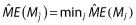, i.e. to find the model that minimizes the model error over all the models. They evaluated complete cross-validation, V-fold cross-validation, the bootstrap and partial cross-validation, and concluded the following: complete cross-validation is too computationally expensive; partial cross-validation is biased and should not be entertained; and V-fold cross-validation and the bootstrap performed well.

Sauerbrei and Schumacher discuss combining a bootstrap method with stepwise procedures [58]. Shao [59] discussed the bootstrap variable selection from a theoretical viewpoint. In Shao's work, a correct model was defined as any model containing the ‘true’ model, because the predictions were unbiased. He showed that variable selection using the bootstrap as typically performed did not lead to consistent model selection as the sample size increased (that is, the procedure did not asymptotically approach probability = 1 of selecting the true model). To make the procedure consistent, bootstrap selection should be performed using a smaller number of samples than those contained in the data. We do not know of any use or evaluations of this reduced sampling in GNLMEM. Typically, methods considering prediction error are only used such as in the lasso or used to evaluate models selected by stepwise procedures. One would need to consider the definition of prediction error as well as whether squared error loss is appropriate given that the marginal density of GNLMEM is not expected to be normally distributed.

Discussion

Many authors have provided evidence and commentary regarding how poorly the stepwise procedures can perform, at least for OLS. The all subset regression procedures find the optimal model as defined by the GIC, but this is not necessarily the optimal model with regard to the intended use. Authors frequently discuss failure to select authentic predictors and inclusion of excess noise variables. Derksen and Keselman [16] state that, ‘the data mining approach to model building is likely to result in final models containing a large percentage of noise variables which will be interpreted incorrectly as authentic’. They go on to quote Cohen [60], ‘If you torture the data for long enough, in the end they will confess’. Authors discuss the inflation of confidence in predicting new data. Breiman and Spector [57] focus on the poor predictability of ‘fixed path’ procedures and their overoptimism. They also state that much of the optimality of the penalties discussed above is nullified when variable selection is data driven. In the end they conclude, ‘We hope this present simulation will drive another nail into the practice of using fixed path estimators when data driven submodel selection is in operation’. Finally, Harrell Jr [15] writes, ‘Stepwise variable selection has been a very popular technique for many years but if this procedure had just been proposed as a statistical method, it would likely be rejected because it violates every principle of statistical estimation and hypothesis testing’.

Despite these harrowing remarks, stepwise methods are still popular today. We feel that this is probably due to the fact these are easy to understand and implement (automate). In fairness, it should be noted that many of the early evaluations in OLS were done with small sample sizes (∼200 observations) and large predictor-to-observation ratios (∼30–40 predictors). Wiegand [1] evaluated a larger range of sample sizes that included 1000 and 5000 observations. He found at these larger sample sizes that the stepwise procedures demonstrated improvement for selection of true predictors yet continued to select false ones. This suggests at larger sample sizes that selection bias decreases (which is expected). Also, many articles assume that all the potential authentic predictors have been collected. This is unlikely to be the case in pharmacometric work. Experience has shown that often predictors are not sufficient to adjust for differences in response levels across studies. This suggests unexplained study-to-study variability (or heterogeneity) and, in addition to other factors such as study design, casts doubt as to whether all the important predictors were contemplated or collected. It should be noted that subjects are randomized between studies, so one should not anticipate that differences between studies should be negligible. The randomization within a study is what helps to ensure that baseline values between treatment arms will be similar. Few have evaluated the performance of any of these methods with respect to latent or unmeasured covariates that are potentially correlated with those evaluated. This is not to say that the difficulties with stepwise procedures would improve. On the contrary, they would probably worsen, but this is worth keeping in perspective. Ultimately, it is clear that variable selection requires some forethought and planning, because these methods unfortunately generate complex statistical and interpretational issues despite their ease of use.

Based on such results and commentary, many have advocated not performing variable selection at all and retain the full model as the final model [61,62]. This corresponds to penalty = 0 in the GIC. The full model estimates remain unbiased estimates, their confidence intervals have proper coverage critical for inference, and the model results do not suffer from selection bias, which often occurs due to lack of statistical power [63]. The full model approach avoids the potential for abuse often perpetrated by implementation of variable selection. It is easy for the analyst to treat the final model that results from the variable selection procedure as if it were prespecified, i.e. to make inference using the resulting estimates and their confidence intervals or assign P values (from the GIC values) to effects as these enter or exit, establishing importance. In essence, it is easy to use stepwise procedures as if they had the oracle property when clearly they do not.

One cannot help but reflect on the issue of accuracy vs. precision, which is always lurking in analyses. Hocking [14] shows clearly (an intuitive result and assuming one is not using data-driven selection) that including extra variables decreases the precision of the predictions, which balances prediction biases resulting from failing to include authentic predictors. Additionally, Breiman and Spector [57] conclude from their simulation work, ‘The message is clear: You may win big using submodel selection in the x-random case, especially for thin sample sizes and irregular X-distribution’ (note that they are not against variable selection, just certain procedures for it). They go on to state that one can even win more by picking smaller submodels. Such statements appeal to the desire for parsimony. If one always selects the full model as the final model, then one will not need to worry about selection bias and errors associated therewith. But, what errors is one making or will one make in the summary or use of such a model? Questions of which are the ‘most important’ predictors or ‘what factors do we need to worry about’ arise throughout drug development. When one considers how to address these, one needs to think about many issues: for what purpose will this information be used; and in what development stage is the compound (as this affects sample size and the range of and number of predictor variables)? For example, end of phase 3 label negotiations might require different strategies from internal phase 2 decision making. Picking a smaller submodel makes sense when discussing the label. Full models work well for looking at each covariate individually, but are unwieldy (cursed by their dimensionality) and could thus be misused in practice when it comes to finding subpopulations, i.e. groups of patients based on a set of predictors that may require dose adjustment. As predictors are often multiplicative in effect, multiple factors can accumulate to lead to a prediction that is suggestive of a need for altering the dosing strategy. It might be difficult to get agreement or buy-in from stakeholders if the results are difficult to use practically. Simulation from a full model is also cumbersome. Some analysts have advocated that covariates be retained in a model only if their effects are clinically meaningful. For example, one might state that a 15% change in CL is not clinically meaningful for females and remove this effect from the model. This has been advocated to be applied to full models, or even the results of stepwise methods. We did not address this in this article, but comment briefly here. It is easy to find situations in pharmacometric analysis in which nonclinically meaningful effects can predict clinical meaningful differences in responses. For example, if one adds this 15% change in CL to a change also influenced by weight and age, then this could lead to a subpopulation that is over- or underexposed. Subpopulations that require dose adjustment could be composed of many patient factors that could even be correlated. If one eliminates a covariate based on its effect in isolation, the identification of a subpopulation could be misinformed.

If the stepwise methods that are discussed herein are to be used for variable selection, we recommend the following strategy. Before embarking on any modelling procedure we suggest that the investigator fit the full model M_A first and evaluate the stability of the fit, such as calculating the condition numbers from the estimated correlation matrices of the COV to assess the a posteriori correlation. We also suggest calculating these for the entire matrix and the submatrix related to the predictor effects. These condition numbers, in our opinion, provide cursory examination of the flatness of the model surface, which can inform the variable selection strategy. Building a full model is the easiest way to ensure that the data can support the estimation of all the predictor effects before invoking a variable selection procedure, even if the FS procedure is to be used. One cannot expect good results (i.e. minimizing spurious findings) from the FS if the full model is unstable, and if the full model is not assessed, one might be blind to these issues.

One can view model flatness in the context of typical regression. Many regression functions can fit small amounts of data. This is analogous for models. If the model space is flat, many models will appear to fit the data adequately, and small changes in the data could lead one to conclude that one model is better than another. Other factors that contribute to the flatness of the model space are the number of subjects or sample size [1] and the ratio of these to the number of predictor variables [21]. These considerations are of specific interest in time-to-event analyses with low event rates. Harrell Jr [15] provides some rules of thumb for the number of predictors that should be evaluated based on the observed data.

If the model space is flat, one should consider data reduction. First, re-evaluate which predictor–parameter combinations make sense from a clinical perspective. Grouping of effects is another strategy. This can be performed for effects of the same predictor when the parameters are correlated or within the same parameter across predictors when the predictors are correlated. In such a case, one should recognize the limitations of the data or design, and clearly articulate what the implications of these are to any inference one intends to make. Selection bias can take on many apparent forms, such as selecting the wrong predictor effect or selecting the correct predictor on the wrong parameter. Additionally, the selection procedure might not select a predictor on either correlated parameter. This can occur when individually parameters do not have enough information but in combination they do, and this can be an issue for the FS method. This provides greater rationale to group such effects during a search. If an effect is of interest, but the design is such that there is lower power to evaluate it – for example, the range of a continuous predictor is too narrow or the number with a certain categorical predictor (e.g. pharmacogenomic group) is too few – then the covariate could be retained until more data can be incorporated. This will avoid selection bias and concluding that the effect is not influential based on insufficient information to say whether it is influential. Alternatively, one could attempt to evaluate the model size that yields the lowest prediction error and use that number as a guide to determine the amount of predictors that can be evaluated. Such a strategy could be computationally expensive. A more direct evaluation of the flatness of the model space is available by all subset regression, but this is at computational expense.

In certain cases, we advocate performing two variable selection procedures in sequence. For example, it can be of interest to evaluate the effects of concomitant medication in the data. Such predictors can have a fair degree of uncertainty in the collection of the data as well as how to incorporate its effect into the model (usage or categorized by dose amount). Evaluations of these effects are more exploratory in our opinion. We suggest first performing a variable selection procedure investigating the standard set of predictors to obtain a tentative final model, and then adding the concomitant medication predictors to this tentative final model and evaluating them using a second variable selection procedure applied only to the concomitant medication predictors. In this way, one relegates the predictors measured with a greater degree of uncertainty to a secondary evaluation in an attempt to mitigate the influence of these on predictors that do not carry such uncertainty. Ultimately, more consideration upfront of meaningful effect evaluations saves time rationalizing the findings, arbitrarily dismissing such findings or performing ad hoc analyses to ‘save’ the interpretation of the analysis. Clear articulation of the predictors and in which parameter submodels these will be evaluated should be prescribed in the analysis plan.

When presenting the results, we suggest presenting the final model with as much information about competing models as possible. Report the estimates and standard errors for the base, full and final model in one table in the report. We feel that this is extremely important. One can see how the standard errors increase in the full model relative to the base model when adding the effects. This represents the cost of exploration. The estimates of the final model can now be compared with the base and full model to see how sensitive the estimates were to the selection procedure. Hopefully, the estimates in the final model do not change much upon elimination of the other variables, because this would indicate that these are not necessarily robust to the choice of the covariates. One can compare the standard errors from the final model with the full model to see the downward bias that results from the selection procedure. In fact, we recommend using the standard errors from the full model when computing confidence intervals for the final model. This procedure will not fix issues with estimates that are associated with the selection procedure, but will help to resolve the issue with confidence interval size. This is not compatible with confidence intervals from the bootstrap using the percentile method. However, if one bootstraps the full model, then standard errors from the bootstrap could be used to compute the confidence intervals. Wald-based confidence intervals could be computed for the full model and compared with those from the percentile method to attain some level of comfort in the procedure. We would expect for reasonable sample sizes that the two methods would be close.

More evaluation of the final model with respect to the full model could be performed to improve confidence and demonstrate adequacy of the model selection (validation). This can be done internally or externally. One should, however, be conscious of what it means to be predictive. Typically, it means how well the model, built on a sample from a population, predicts another sample from the same population. During drug development, it is not clear that this is a practical definition. In phase 2, healthy volunteers are replaced with patients, who have different characteristics. As the drug development programme expands and approaches phase 3, a greater number of sites spanning diverse ethnic and geographical regions often occurs. Inclusion/exclusion criteria may be relaxed or tightened to facilitate recruitment or enrich the population, anticipating a larger effect. After filing and approval, the drug will no longer be in a controlled setting. Investigators who have modelled double-blinded data and encountered difficulties incorporating open-label extension data can relate to the challenges of extrapolating to a less controlled setting. Additionally, once approved, the population of patients may expand to regions of the predictor space never studied. For these reasons, the performance of model selection techniques and the adequacy of predictions extrapolated to new experimental settings or populations will continue to be a necessary but challenging endeavour for pharmacometricians.

Competing Interests

There are no competing interests to declare.

References

- 1.Wiegand RE. Performance of using multiple stepwise algorithms for variable selection. Stat Med. 2010;29:1647–1659. doi: 10.1002/sim.3943. [DOI] [PubMed] [Google Scholar]
- 2.Efroymson MA. Multiple regression analysis. In: Ralston A, Wilf HS, editors. Mathematical Method for Digital Computers. New York: Wiley; 1960. pp. 191–203. [Google Scholar]
- 3.Hamaker HC. On multiple regression analysis. Stat Neerl. 1962;16:31–56. [Google Scholar]
- 4.Boxenbaum H. Interspecies scaling, allometry, physiological time, and the ground plan of pharmacokinetics. J Pharmacokinet Biopharm. 1982;10:201–227. doi: 10.1007/BF01062336. [DOI] [PubMed] [Google Scholar]
- 5.Hoerl AE, Kennard RW. Ridge regression: biased estimation for non-orthogonal problems. Technometrics. 1970a;12:55–67. [Google Scholar]
- 6.Kendall MG. A Course in Multivariate Analysis. New York, USA: Hafner Publishing Co; 1957. [Google Scholar]
- 7.Massy WF. Principal components regression in exploratory statistical research. J Am Stat Assoc. 1965;560:234–246. [Google Scholar]
- 8.Vonesh EF, Chinchilli VM. Linear and Nonlinear Models for the Analysis of Repeated Measurements. New York, USA: Marcel Dekker Inc; 1997. [Google Scholar]
- 9.Ludden TM, Beal SL, Sheiner LB. Comparison of the Akaike information criterion, the Schwarz criterion and the F test as guides to model selection. J Pharmacokinet Biopharm. 1994;29:431–445. doi: 10.1007/BF02353864. [DOI] [PubMed] [Google Scholar]
- 10.Raftery AE, Madigan D, Hoeting JA. Bayesian model averaging for linear regression models. J Am Stat Assoc. 1997;92:179–191. [Google Scholar]
- 11.Hjort NL, Claeskens G. Frequentist model average estimators. J Am Stat Assoc. 2003;98:879–899. [Google Scholar]
- 12.Kowalski KG, Hutmacher MM. Design evaluation for a population pharmacokinetic study using clinical trial simulations: a case study. Stat Med. 2001a;20:75–91. doi: 10.1002/1097-0258(20010115)20:1<75::aid-sim602>3.0.co;2-c. [DOI] [PubMed] [Google Scholar]
- 13.Wade JR, Beal SL, Sambol NC. Interaction between structural, statistical, and covariate models in population pharmacokinetic analysis. J Pharmacokinet Biopharm. 1994;22:165–177. doi: 10.1007/BF02353542. [DOI] [PubMed] [Google Scholar]
- 14.Hocking RR. The analysis and selection of variables in linear regression. Biometrics. 1976;32:1–49. [Google Scholar]
- 15.Harrell FE., Jr . Regression Modeling Strategies: With Applications to Linear Models, Logistic Regression, and Survival Analysis. New York, USA: Springer; 2001. [Google Scholar]
- 16.Derksen S, Keselman HJ. Backward, forward and stepwise automated subset selection algorithms: frequency of obtaining authentic and noise variables. Br J Math Stat Psychol. 1992;45:265–282. [Google Scholar]
- 17.Hoerl AE, Kennard RW. Ridge regression: applications to non-orthogonal problems. Technometrics. 1970b;12:69–82. [Google Scholar]
- 18.Hutmacher MM, Nestorov I, Ludden T, Zitnik R, Banfield C. Modeling the exposure-response relationship of etanercept in the treatment of patients with chronic moderate to severe plaque psoriasis. J Clin Pharmacol. 2007;47:238–248. doi: 10.1177/0091270006295062. [DOI] [PubMed] [Google Scholar]
- 19.Efron B, Hinkley DV. Assessing the accuracy of the maximum likelihood estimator: observed versus expected fisher information. Biometrika. 1978;65:457–487. [Google Scholar]
- 20.Efron B. Nonparametric standard errors and confidence intervals. Can J Stat. 1981;9:139–172. [Google Scholar]
- 21.Freedman DA. A note on screening regression equations. Am Stat. 1983;37:152–155. [Google Scholar]
- 22.Cox DR, Hinkley DV. Theoretical Statistics. New York, USA: Chapman and Hall; 1974. [Google Scholar]
- 23.Beal SL, Sheiner LB, Boeckmann AJ, editors. NONMEM Users Guides. Ellicott City, USA: Icon Development Solutions; 1989–2006. [Google Scholar]
- 24.Vonesh EF. A note on the use of Laplace's approximation for nonlinear mixed-effects models. Biometrika. 1996;83:447–452. [Google Scholar]
- 25.Wählby U, Jonsson EN, Karlsson MO. Assessment of actual significance levels for covariate effects in NONMEM. J Pharmacokinet Pharmacodyn. 2001;28:231–252. doi: 10.1023/a:1011527125570. [DOI] [PubMed] [Google Scholar]
- 26.Beal SL. Commentary on significance levels for covariate effects in NONMEM. J Pharmacokinet Pharmacodyn. 2002;29:403–410. doi: 10.1023/a:1020909324909. discussion 411–412. [DOI] [PubMed] [Google Scholar]
- 27.Akaike H. A new look at the statistical model identification. IEEE Trans Automatic Control. 1974;19:716–723. [Google Scholar]
- 28.Hurvich CM, Tsai CL. Regression and time series model selection in small samples. Biometrika. 1989;76:297–307. [Google Scholar]
- 29.Schwarz G. Estimating the dimension of a model. Ann Stat. 1978;6:461–465. [Google Scholar]
- 30.Jones RH. Bayesian information criterion for longitudinal and clustered data. Stat Med. 2011;30:3050–3056. doi: 10.1002/sim.4323. [DOI] [PubMed] [Google Scholar]
- 31.Clayton MK, Geisser S, Jennings DE. A comparison of several model selection procedures. In: Goel PL, Zellner A, editors. Studies in Bayesian Econometrics and Statistics. New York, USA: Elsevier; 1986. pp. 425–439. [Google Scholar]
- 32.Laud PW, Ibrahim JG. Predictive model selection. J R Stat Soc B. 1995;57:247–262. [Google Scholar]
- 33.Montgomery DC, Peck EA. Introduction to Linear Regression Analysis. New York, USA: John Wiley and Sons, Inc; 1982. [Google Scholar]
- 34.Mantel N. Why stepdown procedures in variable selection. Technometrics. 1970;15:661–675. [Google Scholar]
- 35.Draper NR, Smith H. Applied Regression Analysis. New York: John Wiley and Sons, Inc; 1981. [Google Scholar]
- 36.Mandema JW, Verotta D, Sheiner LB. Building population pharmacokinetic-pharmacodynamic models. I. models for covariate effects. J Pharmacokinet Biopharm. 1992;20:511–528. doi: 10.1007/BF01061469. [DOI] [PubMed] [Google Scholar]
- 37.Hastie T, Tibshirani R. Generalized additive models. Stat Sci. 1986;3:297–310. doi: 10.1177/096228029500400302. [DOI] [PubMed] [Google Scholar]
- 38.Savic RM, Karlsson MO. Importance of shrinkage in empirical Bayes estimates for diagnostics: problems and solutions. AAPS J. 2009;11:558–569. doi: 10.1208/s12248-009-9133-0. [DOI] [PMC free article] [PubMed] [Google Scholar]
- 39.Jonsson EN, Karlsson MO. Automated covariate model building within NONMEM. Pharm Res. 1998;15:1463–1468. doi: 10.1023/a:1011970125687. [DOI] [PubMed] [Google Scholar]
- 40.Khandelwal A, Harling K, Jonsson EN, Hooker AC, Karlsson MO. A fast method for testing covariates in population PK/PD Models. AAPS J. 2011;13:464–472. doi: 10.1208/s12248-011-9289-2. [DOI] [PMC free article] [PubMed] [Google Scholar]
- 41.Leon-Novelo L, Moreno E, Casella G. Objective Bayes model selection in probit models. Statist Med. 2012;31:353–365. doi: 10.1002/sim.4406. [DOI] [PubMed] [Google Scholar]
- 42.Garside MJ. The best subset in multiple regression analysis. J R Stat Soc Ser C Appl Stat. 1965;14:196–200. [Google Scholar]
- 43.Furnival GM. All possible regressions with less computation. Technometrics. 1971;13:403–408. [Google Scholar]
- 44.Goodnight JH. A tutorial on the SWEEP operator. Am Stat. 1979;33:149–158. [Google Scholar]
- 45.Hocking RR, Leslie RN. Selection of the best subset in regression analysis. Technometrics. 1967;9:531–540. [Google Scholar]
- 46.Furnival GM, Wilson RW., Jr Regression by leaps and bounds. Technometrics. 1974;16:499–511. [Google Scholar]
- 47.Lawless JF, Singhal K. Efficient screening of nonnormal regression models. Biometrics. 1978;34:318–327. [Google Scholar]
- 48.Kowalski KG, Hutmacher MM. Efficient screening of covariates in population models using Wald's approximation to the likelihood ratio test. J Pharmacokinet Pharmacodyn. 2001b;28:253–275. doi: 10.1023/a:1011579109640. [DOI] [PubMed] [Google Scholar]
- 49.Wald A. Tests of statistical hypotheses concerning several parameters when the number of observations is large. Trans Am Math Soc. 1943;54:426–482. [Google Scholar]
- 50.Bies RR, Muldoon MF, Pollock BG, Manuck S, Smith G, Sale ME. A genetic algorithm-based, hybrid machine learning approach to model selection. J Pharmacokinet Pharmacodyn. 2006;33:195–221. doi: 10.1007/s10928-006-9004-6. [DOI] [PubMed] [Google Scholar]
- 51.Sherer EA, Sale ME, Pollock BG, Belani CP, Egorin MJ, Ivy PS, Lieberman JA, Manuck SB, Marder SR, Muldoon MF, Scher HI, Solit DB, Bies RR. Application of a single-objective, hybrid genetic algorithm approach to pharmacokinetic model building. J Pharmacokinet Pharmacodyn. 2012;39:393–414. doi: 10.1007/s10928-012-9258-0. [DOI] [PMC free article] [PubMed] [Google Scholar]
- 52.Tibshirani R. Regression shrinkage and selection via the lasso. J R Stat Soc B. 1996;58:267–288. [Google Scholar]
- 53.Ribbing J, Nyberg J, Caster O, Jonsson EN. The lasso – a novel method for predictive covariate model building in nonlinear mixed effects models. J Pharmacokinet Pharmacodyn. 2007;34:485–517. doi: 10.1007/s10928-007-9057-1. [DOI] [PubMed] [Google Scholar]
- 54.Tibshirani R. The lasso method for variable selection in the Cox model. Stat Med. 1997;16:385–395. doi: 10.1002/(sici)1097-0258(19970228)16:4<385::aid-sim380>3.0.co;2-3. [DOI] [PubMed] [Google Scholar]
- 55.Fan J, Li R. Variable selection via nonconcave penalized likelihood and its oracle properties. J Am Stat Assoc. 2001;96:1348–1360. [Google Scholar]
- 56.Lunn DJ. Automated covariate selection and Bayesian model averaging in population PK/PD models. J Pharmacokinet Pharmacodyn. 2008;35:85–100. doi: 10.1007/s10928-007-9077-x. [DOI] [PubMed] [Google Scholar]
- 57.Breiman L, Spector P. Submodel selection and evaluation in regression – the X-random case. Int Stat Rev. 1992;60:291–319. [Google Scholar]
- 58.Sauerbrei W, Schumacher M. A bootstrap resampling procedure for model building: application to the Cox regression model. Stat Med. 1992;11:2093–2109. doi: 10.1002/sim.4780111607. [DOI] [PubMed] [Google Scholar]
- 59.Shao J. Bootstrap model selection. J Am Stat Assoc. 1996;91:655–665. [Google Scholar]
- 60.Cohen J. Things I have learned (so far) Am Psychol. 1990;45:1304–1312. [Google Scholar]
- 61.Gastonguay M. 2011. Full covariate models as an alternative to methods relying on statistical significance for inferences about covariate effects: a review of methodology and 42 case studies. PAGE 20, Abstr 2229. Available at http://www.page-meeting.org/?abstract=2229 (last accessed 16 July 2014)
- 62.Hu C, Zhang J, Zhou H. Confirmatory analysis for phase III population pharmacokinetics. Pharm Stat. 2011;10:14–26. doi: 10.1002/pst.403. [DOI] [PubMed] [Google Scholar]
- 63.Steyerberg EW, Eijkemans MJC, Habbema JDF. Stepwise selection in small data sets: a simulation study of bias in logistic regression analysis. J Clin Epidemiol. 1999;52:935–942. doi: 10.1016/s0895-4356(99)00103-1. [DOI] [PubMed] [Google Scholar]