Quartet Inference from SNP Data Under the Coalescent Model

Abstract

Motivation: Increasing attention has been devoted to estimation of species-level phylogenetic relationships under the coalescent model. However, existing methods either use summary statistics (gene trees) to carry out estimation, ignoring an important source of variability in the estimates, or involve computationally intensive Bayesian Markov chain Monte Carlo algorithms that do not scale well to whole-genome datasets.

Results: We develop a method to infer relationships among quartets of taxa under the coalescent model using techniques from algebraic statistics. Uncertainty in the estimated relationships is quantified using the nonparametric bootstrap. The performance of our method is assessed with simulated data. We then describe how our method could be used for species tree inference in larger taxon samples, and demonstrate its utility using datasets for Sistrurus rattlesnakes and for soybeans.

Availability and implementation: The method to infer the phylogenetic relationship among quartets is implemented in the software SVDquartets, available at www.stat.osu.edu/∼lkubatko/software/SVDquartets.

Contact: lkubatko@stat.osu.edu

Supplementary information: Supplementary data are available at Bioinformatics online.

1 INTRODUCTION

With recent advances in DNA sequencing technology, it is now common to have available alignments from multiple genes for inference of an overall species-level phylogeny. While this species tree is generally the object that we seek to estimate, it is widely known that each individual gene has its own phylogeny, called a gene tree, which may not agree with the species tree. Many possible causes of this gene incongruence are known, including horizontal gene transfer, gene duplication and loss, hybridization and incomplete lineage sorting (Maddison, 1997). Of these, the best studied is incomplete lineage sorting, which is commonly modeled by the coalescent process (Kingman, 1982a,b; Liu et al., 2009a). Much recent effort has been devoted to the development of methods to estimate species-level phylogenies from multi-locus data under the coalescent model (Bryant et al., 2012; Heled and Drummond, 2010; Kubatko et al., 2009; Liu and Pearl, 2007; Liu et al., 2009b; Than and Nakhleh, 2009).

Here, we consider this basic problem, although our approach to the problem differs from previous approaches in several important ways. Previous approaches can be divided into two groups (Liu et al., 2009a): summary-statistics approaches and sequence-based approaches. Summary-statistics approaches first estimate a gene tree independently for each gene, and then treat the estimated gene trees as data for a second stage of analysis to estimate the species tree. The most popular approaches in this category are Maximum Tree (Liu et al., 2009b) [also implemented in the program STEM (Kubatko et al., 2009)], STAR (Liu et al., 2009c), STEAC (Liu et al., 2009c), MP-EST (Liu et al., 2010) and Minimize Deep Coalescences [as implemented in the program PhyloNet (Than and Nakhleh, 2009)]. These methods are computationally efficient for large datasets, but generally ignore variability in the estimated gene trees and thus potentially lose accuracy. The second group of methods uses the full data for estimation of the species tree via a Bayesian framework for inference. The three most common methods in this group, BEST (Liu and Pearl, 2007), *BEAST (Heled and Drummond, 2010) and SNAPP (Bryant et al., 2012), all seek to estimate the posterior distribution for the species tree using Markov chain Monte Carlo (MCMC), but differ in some details of the implementation. These methods become time-consuming when the number of loci is large, and assessment of convergence of the MCMC can be difficult.

Our proposed method is distinct from both classes of existing approaches in that it uses the full data directly, but does not utilize a Bayesian framework. It is thus computationally efficient while incorporating all sources of variability (both mutational variance and coalescent variance (cf. Huang et al., 2010) in the estimation process. The theory underlying our method applies to unlinked single nucleotide polymorphism (SNP) data, for which each site is assumed to have its own genealogy drawn from the coalescent model; however, we use simulation to show that the method also performs well for multi-locus sequence data. To describe our proposed method, we first begin with a brief overview of the coalescent model in the context of species-level phylogenetics. We use simulation to assess the performance of the method for both simulated and empirical data. We conclude with a short discussion of how the proposed method can be scaled up to larger taxon sets for estimation of species phylogenies in a coalescent framework, and apply it to two empirical datasets.

1.1 Site pattern probability distributions under the coalescent model

The coalescent model can be used to compute the probability distribution of gene trees given a particular species tree and set of speciation times (which determine species tree branch lengths). Both the discrete probability distribution on the space of gene tree topologies (Degnan and Salter, 2005) and the probability density on the space of gene trees with branch lengths (Rannala and Yang, 2003) have been derived recently. Using these probability distributions, it is possible to compute the probability distribution on data patterns at the tips of a species tree. Let X_H be the observed state in the data at tip H, and, referring to the tree in Figure 1, for example, define p_ijkl as

$$p_{ijkl}=P(X_1=i,X_2=j,X_3=k,X_4=l).$$ (1)

for $i,j,k,l\in \{A,C,G,T\}$. To compute the probability distribution $\left\{p_{ijkl}\right|i,j,k,l\in \{A,C,G,T\}\}$, we need the following: (i) a species phylogeny, with speciation times specified; and (ii) a model for sequence evolution along a gene tree, e.g. the General Time-Reversible (GTR) model (Tavare, 1986) or the Jukes–Cantor (JC69) model (Jukes and Cantor, 1969). See DeGiorgio and Degnan (2010) for an example of how to carry out this computation for a two-state model. The details of the calculation for arbitrary k-state models can be found in Chifman and Kubatko (2014). We now describe how this probability distribution can be used to compute a score on a quartet of taxa that can identify the true quartet relationship. To begin, we define a split of a phylogenetic tree as follows.

Definition —

A split of a set of taxa $\mathcal{L}$ is a bipartition of $\mathcal{L}$ into two non-overlapping subsets L₁ and L₂, denoted $L_1|L_2$. A split $L_1|L_2$ is valid for tree T if the subtrees containing the taxa in L₁ and in L₂ do not intersect.

For a quartet of taxa, we consider splits for which $\left|L_1\right|=2$ (and thus necessarily $\left|L_2\right|=2$), e.g., we consider splitting the four taxa into two groups of two. For example, consider a valid split $L_1|L_2$, where $L_1=\{1,2\}$ and $L_2=\{3,4\}$ (Fig. 1). Under this partition, we can display the probability distribution $P=\left\{p_{ijkl}\right|i,j,k,l\in \{A,C,G,T\}\}$ in the form of a flattening along a split $L_1|L_2$, denoted by $Fla{t}_{L_1|L_2}(P)$, as follows:

$$\left(\begin{array}{ccccccc}{p}_{AAAA}& p_{AAAC}& p_{AAAG}& p_{AAAT}& p_{AACA}& \dots & p_{AATT}\\ p_{ACAA}& p_{ACAC}& p_{ACAG}& p_{ACAT}& p_{ACCA}& \dots & p_{ACTT}\\ p_{AGAA}& p_{AGAC}& p_{AGAG}& p_{AGAT}& p_{AGCA}& \dots & p_{AGTT}\\ p_{ATAA}& p_{ATAC}& p_{ATAG}& p_{ATAT}& p_{ATCA}& \dots & p_{ATTT}\\ p_{CAAA}& p_{CAAC}& p_{CAAG}& p_{CAAT}& p_{CACA}& \dots & p_{CATT}\\ ⋮& ⋮& ⋮& ⋮& ⋮& \ddots & ⋮\\ p_{TTAA}& p_{TTAC}& p_{TTAG}& p_{TTAT}& p_{TTCA}& \dots & p_{TTTT}\end{array}\right).$$

Fig. 1.

Example four-taxon phylogeny. Split $12|34$ is valid, as the subtree consisting of taxa 1 and 2 does not overlap the subtree consisting of taxa 3 and 4. The two non-valid splits for this tree are $13|24$ and $14|23$

In the above $16\times 16$ matrix, the rows correspond to the possible nucleotides for the two taxa in set L₁ and the columns correspond to the possible nucleotides for the two taxa in set L₂. For more information about flattening of a tensor P for the general Markov model on a gene tree, see Allman and Rhodes (2008). Using this representation, we make use of the following result for species tree inference under the coalescent.

Theorem 1 [Chifman and Kubatko, 2014] —

Let $\mathcal{C}$ denote the class of coalescent models under the four-state GTR model on a four-taxon binary species tree. For a valid split $L_1|L_2$, rank($Fla{t}_{L_1|L_2}(P)$) $\le 10$ for all distributions P arising from $\mathcal{C}$. For a non-valid split $L_1|L_2$, generically, rank($Fla{t}_{L_1|L_2}(P)$) > 10.

We note that the above theorem implies generic identifiability of the unrooted species tree topology for four taxa under the coalescent model (Chifman and Kubatko, 2014). By ‘generic’ we mean that the set of parameters on which the model is non-identifiable is a subset of a proper subvariety of measure zero. In addition, we have established generic identifiability of the unrooted n-taxon species tree under the coalescent model from the induced quartets (Chifman and Kubatko, 2014).

2 METHODS

2.1 Inferring splits using singular value decomposition

Our goal is to use the result of Theorem 1 to infer species phylogenies. Assume that the available data consist of a large sample of unlinked SNPs, which we can used to construct an estimate of the matrix $Fla{t}_{L_1|L_2}(P)$. We call this matrix $Fla{t}_{L_1|L_2}(\widehat{P})$, and define this matrix by

$$\left(\begin{array}{ccccccc}{\widehat{p}}_{AAAA}& {\widehat{p}}_{AAAC}& {\widehat{p}}_{AAAG}& {\widehat{p}}_{AAAT}& {\widehat{p}}_{AACA}& \dots & {\widehat{p}}_{AATT}\\ {\widehat{p}}_{ACAA}& {\widehat{p}}_{ACAC}& {\widehat{p}}_{ACAG}& {\widehat{p}}_{ACAT}& {\widehat{p}}_{ACCA}& \dots & {\widehat{p}}_{ACTT}\\ {\widehat{p}}_{AGAA}& {\widehat{p}}_{AGAC}& {\widehat{p}}_{AGAG}& {\widehat{p}}_{AGAT}& {\widehat{p}}_{AGCA}& \dots & {\widehat{p}}_{AGTT}\\ {\widehat{p}}_{ATAA}& {\widehat{p}}_{ATAC}& {\widehat{p}}_{ATAG}& {\widehat{p}}_{ATAT}& {\widehat{p}}_{ATCA}& \dots & {\widehat{p}}_{ATTT}\\ {\widehat{p}}_{CAAA}& {\widehat{p}}_{CAAC}& {\widehat{p}}_{CAAG}& {\widehat{p}}_{CAAT}& {\widehat{p}}_{CACA}& \dots & {\widehat{p}}_{CATT}\\ ⋮& ⋮& ⋮& ⋮& ⋮& \ddots & ⋮\\ {\widehat{p}}_{TTAA}& {\widehat{p}}_{TTAC}& {\widehat{p}}_{TTAG}& {\widehat{p}}_{TTAT}& {\widehat{p}}_{TTCA}& \dots & {\widehat{p}}_{TTTT}\end{array}\right),$$

where ${\widehat{p}}_{ijkl}$ is the frequency with which we observe the event $\{X_1=i,X_2=j,X_3=k,X_4=l\}$ in the data where $L_1=\{1,2\}$ and $L_2=\{3,4\}$. A key observation is that this can be rapidly tabulated for quartets of taxa even for datasets of very large size.

We want to infer which of the three possible splits on quartets is the true split. One way to assess this would be to consider the $Fla{t}_{L_1|L_2}(\widehat{P})$ matrix for each of the three possible splits, and measure which of the three is closest to a rank 10 matrix. To do this, we need a method to measure distances between matrices. Our choice of a distance, described below, is modeled after the approach of Eriksson (2005), who considered the problem of tree estimation from a flattening matrix obtained from the probability distribution of site patterns at the tips of a gene tree. His overall approach to estimation of the phylogeny differed from ours; however, in that he used splits of varying sizes (rather than just splits of quartets of taxa) to develop a clustering algorithm to obtain the phylogenetic estimate. We provide the details of our approach below.

Let a_ij be the ${(i,j)}^{th}$ entry of an $m\times n$ matrix A. The Frobenius norm of a matrix A is

$$\left|\right|A|{|}_F=\sqrt{{\displaystyle \sum _{i=1}^m{\displaystyle \sum _{j=1}^n{a}_{ij}^2}}}.$$

An important property of the Frobenius norm is its characterization using the singular values of A, that is

$$\left|\right|A|{|}_F=\sqrt{{\displaystyle \sum _{i=1}^p{\sigma }_i^2}},$$

where ${\sigma }_1\ge {\sigma }_2\ge \dots \ge {\sigma }_p\ge 0$ are the singular values of A and $p=\text{min}\{m,n\}$.

The well-known low-rank approximation theorem (Eckart–Young theorem) implies that the distance from a matrix A to the nearest rank k matrix in the Frobenius norm is

See Section 2.4 in Golub and Van Loan (2013) for more information about singular value decomposition.

We apply this well-known result to our species tree estimation problem by defining the SVD score for a split $L_1|L_2$ to be

$$SVD(L_1|L_2):=\sqrt{{\displaystyle \sum _{i=11}^{16}{\widehat{\sigma }}_i^2}},$$ (2)

where $\widehat{{\sigma }_i}$ are the singular values of $Fla{t}_{L_1|L_2}(\widehat{P})$ for $i\in \{11,\dots ,16\}$. Our proposal for inferring the true species-level relationship within a sample of four taxa is thus the following. For each of the three possible splits, construct the matrix $Fla{t}_{L_1|L_2}(\widehat{P})$ and compute SVD $(L_1|L_2)$. The split with the smallest score is taken to be the true split.

To quantify uncertainty in the inferred split, we implement a nonparametric bootstrap procedure as follows. For a dataset consisting of Maligned sites, we re-sampled the columns of the data matrix with replacement M times to generate a new bootstrapped data matrix, and the SVD scores of the three splits are computed for this bootstrapped data matrix. This procedure is repeated B times, and the proportion of bootstrapped datasets that support each of the three possible splits provides a measure of support for that split.

2.2 Simulation study

We first use simulated data to assess the ability of SVD $(L_1|L_2)$ to correctly identify the valid split under a variety of conditions. Before describing the simulation procedure, we first point out that while much of the currently available methodology for inferring species trees assumes that multi-locus data (e.g. aligned DNA sequences from many independent loci) are available for inference, our method is actually designed for unlinked sites, for example, for a sample of unlinked SNPs. This is because in computing the probability distribution of site patterns at the tips of the species tree, we integrate over the probability distribution of gene trees under the coalescent model, with the implicit assumption that sequence data evolve along these gene trees. Thus each site pattern is viewed as an independent draw from the distribution $f(X_1=i,X_2=j,X_3=k,X_4=l|S)={\int }_{G}f(X_1=i,X_2=j,X_3=k,X_4=l|G)f(G|S)dG$, where S represents the species tree (topology and speciation times) and G represents a gene tree (both topology and divergence times). True multi-locus data, however, consist of an aligned portion of the DNA that is believed to share a single underlying gene tree, and thus all sequence data within a locus are believed to have evolved from a common gene genealogy.

We wish to examine the performance of our method for both unlinked SNP data and for multi-locus data, and we thus consider simulated data of two types: unlinked SNP data (e.g. each site has its own underlying gene tree) and multi-locus data (a sequence of length l is simulated from a shared underlying gene tree). Our simulation consists of the following steps:

1. Generate a sample of g gene trees from the model species tree ((1:x,2:x):x,(3:x,4:x):x), where x is the length of each branch under the coalescent model using the program COAL (Degnan and Salter, 2005).

2. Generate sequence data of length n on each gene tree under a specified substitution model using the program Seq-Gen (Rambaut and Grassly, 1997).

3. Construct the flattening matrix for each of the three possible splits, and compute SVD $(L_1|L_2)$ for each.

4. Repeat the above procedure (Steps 1–3) 1000 times and record SVD ${(L_1|L_2)}_k,k=1,2,\dots ,1000$, for each split. For each of the 1000 datasets, generate B bootstrapped datasets and record SVD ${(L_1|L_2)}_{k,b},k=1,2,\dots ,1000;b=1,2,\dots ,B$ for each split.

Given the above simulation algorithm, there are several choices to be made at each step. In step (1), we must select the lengths of the branches, x, in the model species tree. We considered branches of length 0.5, 1.0 and 2.0 coalescent units. A branch of length 0.5 coalescent units is very short, and corresponds to a case in which there will be widespread incomplete lineage sorting, making species tree inference difficult. A branch of length 2.0 coalescent units is longer and will result in much lower rates of incomplete lineage sorting, resulting in an easier species tree inference problem.

In step (2), we need to choose the gene length, n. In simulating unlinked SNP data, we used g = 5000 and n = 1 (corresponding to 5000 unlinked SNPs) and for the multi-locus setting, we considered g = 10 and n = 500 (corresponding to 10 genes, each of length 500 sites). Further, step (2) requires choice of substitution model to be used to simulate sequence data on the sampled gene trees. We considered two possibilities: the Jukes–Cantor model (JC69) (Jukes and Cantor, 1969) and the GTR model with a proportion of invariant sites and with gamma-distributed mutation rates across sites (GTR + I + Γ) (Tavare, 1986). In particular, we use the Seq-Gen options -mGTR -r 1.0 0.2 10.0 0.75 3.2 1.6 -f 0.15 0.35 0.15 0.35 -i 0.2 -a 5.0 -g 3 to simulate under GTR + I + Γ. Because the theoretical results in Section 2.1 were derived under the GTR model and associated sub-models (such as JC69), we expect our method to handle the JC69 case well. However, we have not derived results under models in which there are invariant sites or rate variation among sites, so the simulations under the GTR + I + Γ setting will test robustness of the method to these evolutionary processes. In Step (4), we set B = 100.

We carry out one additional simulation to examine the ability of the method to identify the true split for varying overall dataset sizes. We consider unlinked SNP data with 1000, 5000 or 10 000 sites ($g=1000,5000$ or 10 000 and n = 1 in all cases). We used the JC69 model and considered branch lengths of $x=0.5,1.0,$ and 2.0. We recorded the time it took to carry out each of these simulations to assess how computation time scales with the size of the dataset.

2.3 Application to rattlesnake data

We have also explored the use of our quartet inference method in constructing larger species-level phylogenies, and we show here the results of applying the method to a dataset consisting of 19 genes sampled in 26 rattlesnakes from four distinct species: Sistrurus catenatus (with subspecies S. c. catenatus, S. c. edwardsii, and S. c. tergeminus); Sistrurus miliarius (with subspecies S. m. miliarius, S. m. barbouri, and S. m. streckeri); and two outgroup species, Agkistrodon contortrix and Agkistrodon piscivorus. This dataset has been previously analyzed by Kubatko et al. (2011), and details concerning the loci used and the assembly of the aligned data matrix can be found there. Here, we note that the sequences were computationally phased, so that each individual is represented by two distinct sequences in the dataset, for a total of 52 sequences and 8466 aligned nucleotide positions in the complete data matrix.

To conduct the analysis, we randomly sampled 20 000 quartets from the 52 sequences, and used the SVD score to infer the true quartet relationship for each sampled quartet. The quartet assembly program Quartet MaxCut (Snir and Rao, 2012) was used to construct phylogenies from the inferred quartets in two ways. First, a lineage tree was constructed by direct application of Quartet MaxCut. Second, a species-level phylogeny was constructed by replacing the labels of the lineages for the sampled quartets with the subspecies to which they belonged prior to application of Quartet MaxCut. Finally, a bootstrap analysis was carried out by generating 100 bootstrapped datasets from the original matrix and applying this entire procedure to each bootstrapped dataset. The complete analysis, including data simulation, bootstrapping and quartet assembly, took ∼23 h in serial on a desktop Linux machine (2 × Quad Core Xeon E5520/2.26GHz/32GB).

2.4 Application to soybean data and comparison to SNAPP

To demonstrate the utility of our method further, we used a previously published dataset consisting of 17 wild soybean types (Glycine soja) and 14 cultivated soybean types (Glycine max) with 6 289 747 SNP loci. The original analysis was performed by Lam et al. (2010), and the data were later reanalyzed by Lee et al. (2014). We also carried out computations in SNAPP (Bryant et al., 2012), which is suitable for the soybean dataset as it consists of SNP (rather than multi-locus) data, to compare the run times. SNAPP infers the species tree using the coalescent model and is designed for biallelic data consisting of unlinked SNPs (Bryant et al., 2012). Even though our extended SVDquartets method to infer species trees can handle the entire dataset, including missing data, to make a proper and fair comparison with SNAPP, we have removed all missing data and ambiguous sites, resulting in 1 027 026 SNP loci. We also subsampled 10 of the 31 species (four cultivars and six wild types) to run the analysis in SNAPP in a feasible time frame. The formatted datasets used for the analyses with SNAPP and SVDquartets are given in Supplemental Files 2 and 3, respectively. We conducted the analysis using SVDquartets in an analogous way to that for the rattlesnakes, with 20 000 quartets sampled and 100 bootstrap replicates.

3 IMPLEMENTATION

We have written a program in the C language, SVDquartets, which will compute SVD $(L_1|L_2)$ for the three possible splits in a sample of four taxa. The program takes as its input an alignment of four taxa in PHYLIP format, and produces a file that contains a list of the three splits and their associated scores. The program is available from http://www.stat.osu.edu/∼lkubatko/software/SVDquartets/.

4 RESULTS AND DISCUSSION

4.1 Simulation study

Figures 2 and 3 show boxplots of the SVD scores for each of the three possible splits among four taxa under various simulation conditions. It is immediately clear that in all cases the SVD score can easily differentiate between the valid and non-valid splits, with the boxplot corresponding to the valid split displaying scores that are uniformly lower than the scores for the non-valid splits. The separation of scores for valid versus non-valid splits becomes more pronounced as the branch lengths in the species tree increase, as expected, and is, in general, greater for the unlinked SNP data than for the multi-locus data, although the separation is very clear even for the multi-locus data.

Fig. 2.

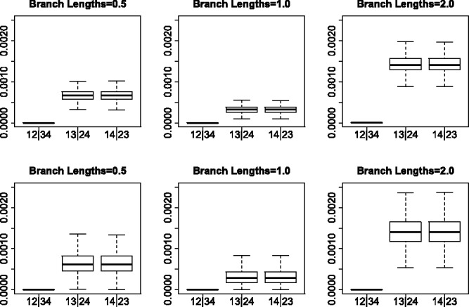
Simulation results for the JC69 model. The top row gives the results for 5000 unlinked SNP sites and the bottom row gives the results for 10 genes with 500 sites each. The columns correspond to differing branch lengths in the model species tree. The first boxplot in each subfigure shows the distribution of SVD scores for the true split, while the next two boxplots show the distribution for the two false splits

Fig. 3.

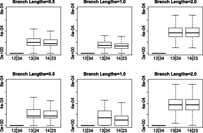
Simulation results for the GTR + I + Γ model. The top row gives results for 5000 unlinked SNP sites and the bottom row gives the results for 10 genes with 500 sites each. The columns correspond to differing branch lengths in the model species tree. The first boxplot in each subfigure shows the distribution of SVD scores for the true split, while the next two boxplots show the distribution for the two false splits

Similarly, the JC69 model with no invariant sites and no rate variation across sites provides the best separation of scores between valid and non-valid splits. The worst performance observed was for the simulation conditions in which the data were simulated under GTR + I + Γ in the multi-locus setting, which is not unexpected as this violates the theoretical conditions in two ways (the invariant sites and variable rates across sites and the multi-locus rather than unlinked SNP data). However, even in this case, the separation in scores is clear, and with sufficiently long species tree branch lengths, there is essentially no overlap in scores in valid versus non-valid splits.

Figures 4 and 5 show boxplots of the bootstrap support values associated with each of the three splits under all simulation conditions. In the case of the JC69 model (Fig. 4), the true split is nearly always associated with 100% bootstrap support for both unlinked SNP data and for multi-locus data. For data simulated under the GTR + I + Γ model, however, bootstrap support values for the true split are sometimes lower, with the worst results occurring when the branch lengths are short. Overall, however, the bootstrap appears to give a reliable measure of support for the true split, particularly when the model assumptions are satisfied.

Fig. 4.

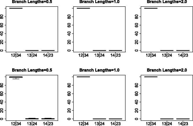
Bootstrap results for the JC69 model simulations. Each boxplot shows the distribution of the bootstrap support values for each of the three possible splits for the simulated data shown in Figure 2

Fig. 5.

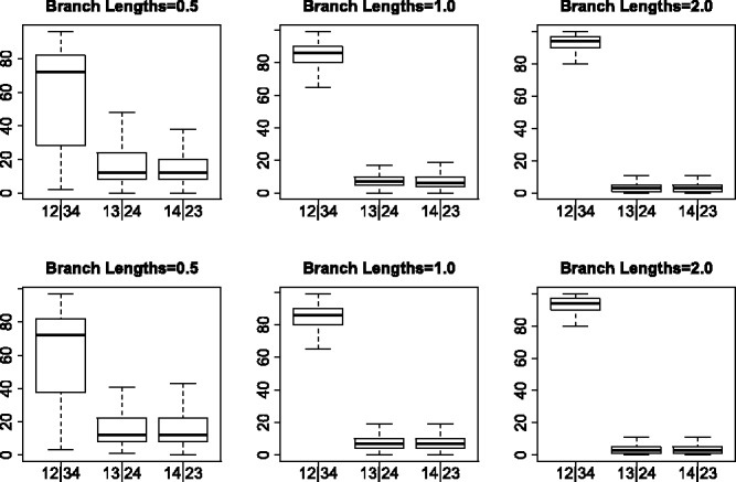
Bootstrap results for the GTR + I + Γ simulations. Each boxplot shows the distribution of the bootstrap support values for each of the three possible splits for the simulated data shown in Figure 3

Figure 6 examines the performance of the method for unlinked SNP data with varying numbers of sites. In particular, unlinked SNP datasets were generated with 1000, 5000 or 10 000 total sites under model species trees with branch lengths of 0.5, 1.0 or 2.0 coalescent units. These results demonstrate that the method performs well even for smaller sample sizes. However, it is clear that as the sample size becomes larger, the separation between the scores for the valid and non-valid splits increases. This is to be expected, because the matrix $Fla{t}_{L_1|L_2}(\widehat{P})$ will better approximate $Fla{t}_{L_1|L_2}(P)$ for larger sample sizes.

Fig. 6.

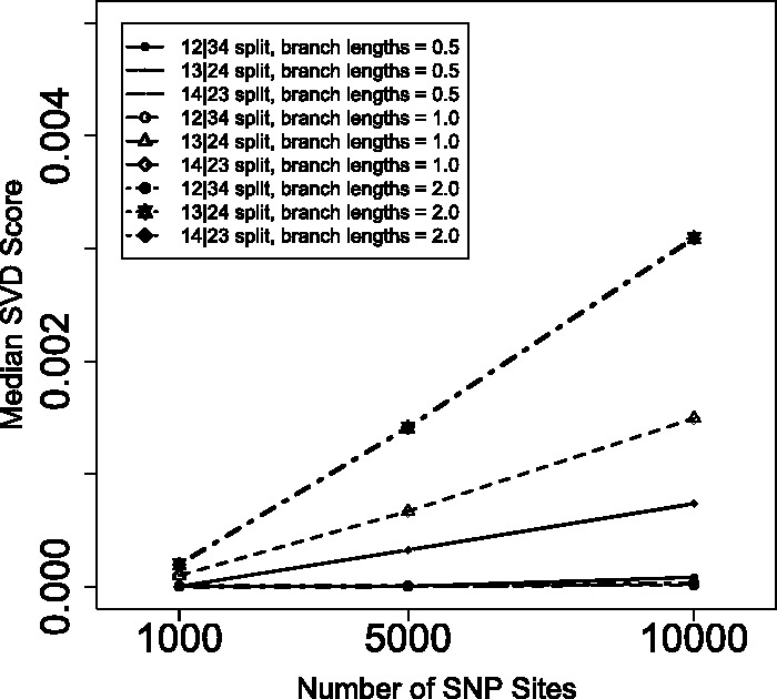
Simulation results for data consisting of 1000, 5000 or 10 000 unlinked SNP sites for trees with branch lengths of 0.5 coalescent units (solid lines), 1.0 coalescent units (dashed lines) or 2.0 coalescent units (dotted lines). The median SVD score (taken over 1000 replicates) for the valid split $12|34$ are marked with circles, while the scores for the two non-valid splits are marked with triangles and diamonds.

Table 1 gives timing results for the simulations carried out in Figure 6. Because the main work undertaken by the method involves counting the number of site patterns to build the $Fla{t}_{L_1|L_2}(\widehat{P})$ matrix, the time should be approximately linear in the number of unique site patterns in the data, which is related to both the total number of sites in the data matrix and the overall scale of time represented by the phylogeny. The results in Table 1 demonstrate that the time is less than linear in the total number of site patterns, as expected, and that the computations can be carried out very rapidly (e.g. the computation of three SVD scores for data matrices of 10 000 sites takes <0.1 s).

Table 1.

Time information for the simulation study with results shown in Figure 6

Branch lengths	Number of sites	Real time	User time	System time
0.5	1000	0.0495	0.0092	0.0075
0.5	10 000	0.0566	0.0155	0.0077
1.0	1000	0.0502	0.0105	0.0074
1.0	10 000	0.0564	0.0163	0.0076
2.0	1000	0.0500	0.0119	0.0061
2.0	10 000	0.0553	0.0173	0.0064

Note. All results represent the average time in seconds (over 1000 replicates) to carry out the computation of three SVD scores for the simulated datasets, and were obtained using the UNIX $\mathrm{time}$ command.

4.2 Potential use for species tree inference

These results make it clear that the SVD score is a highly accurate means of inferring the correct, unrooted phylogenetic tree among a set of four taxa. We note that the SVD score is extremely easy to compute. It requires only counting the site patterns and constructing the matrix $Fla{t}_{L_1|L_2}(\widehat{P})$. Computing singular values of a $16\times 16$ matrix is a standard calculation that any mathematical or statistical software package can easily implement. Our software, SVDquartets, carries out both steps using a PHYLIP-formatted input file.

Given the efficiency with which computations can be carried out in the four-taxon setting, this method is a good candidate for estimation of species trees for larger taxon sets. We propose that the method could be used in the following way. For a dataset with T taxa, form all samples of four taxa, or sample sets of four taxa if T is large. For each sample of four taxa, infer the valid split using the SVD score. Using the collection of inferred valid splits, construct a species tree estimate using a quartet assembly method. Substantial previous work and software exist for the problem of quartet assembly (see, e.g. Snir and Rao, 2012; Strimmer and von Haeseler, 1996; Strimmer et al., 1997). We give the results of using this method for inferring a tree consisting of several North American rattlesnake species and for inferring a tree from SNP data for several soybean species below.

This method has tremendous potential to improve the set of tools available for species tree inference. Unlike summary statistics methods, which are known to be quick but fail to model variability in individual gene tree estimates, this method uses the sequence data directly, thus incorporating all sources of variability. The other existing methods based on sequence data (BEST, *BEAST and SNAPP) all rely on Bayesian MCMC methods, and thus require long computing times and the difficult problem of assessing convergence. Our method can be carried out rapidly, and is easily parallelizable, as each quartet can be analyzed on a separate processor. Our method can handle both unlinked SNP and multi-locus data, again providing an advantage over existing sequence-based methods, which can handle either SNP (SNAPP) or multi-locus (BEST and *BEAST) data. Bootstrapping can be easily implemented to provide a means of quantifying support for the estimated phylogeny.

However, there are several issues with this method that will need to be examined in future work. First, the number of quartets to be sampled needs to be specified in cases where the number of taxa is too large to examine all possible quartets. This number should necessarily increase with increasingly large taxon samples, but we have not yet rigorously examined how to select this. In addition, it is worth pointing out that the method only estimates the topology. In some studies, other parameters associated with the evolutionary process, such as branch lengths and effective population sizes, will also be of interest. One possibility is that the tree topology could first be estimated with this method, and then fixed in a subsequent MCMC analysis with either *BEAST or SNAPP, thus greatly reducing the complexity of that analysis. Finally, we have not yet conducted a thorough simulation study of the inferential accuracy of this method for full species tree inference, which will be the topic of future work.

4.3 Application to rattlesnake data

The results of the analysis of the rattlesnake dataset are shown in Figure 7, with bootstrap support values >50% indicated on the appropriate nodes. In the case of the lineage tree (Fig. 7a), the method identifies the two major species S. catenatus and S. miliarius with high bootstrap support, and additionally groups the subspecies S. c. catenatus as monophyletic. In the species tree in Figure 7b, we again see that the method correctly identifies the two species with high bootstrap support, and is able to differentiate subspecies S. c. catenatus from a clade containing the other two subspecies within this group. Within the species S. miliarius, there is not strong support for the subspecies relationships.

Fig. 7.

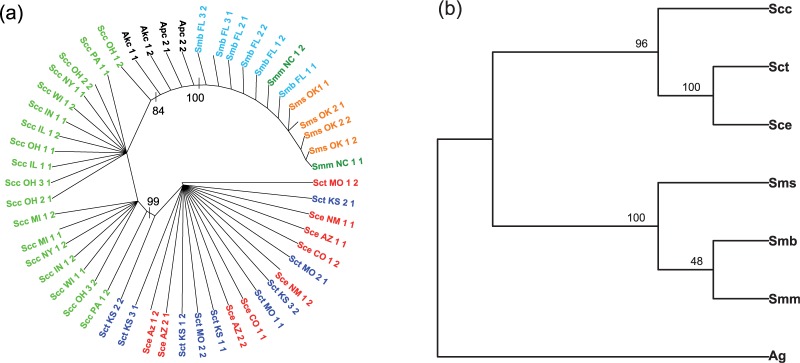
Results of the analysis of the rattlesnake data. In (a), the tree relating all 52 lineages is shown. Colors indicate subspecies membership: Scc = S. c. catenatus (green); Sce = S. c. edwardsii (red); Sct = S. c. tergeminus (blue); Smm = S. m. miliarius (dark green); Sms = S. m. streckeri (orange); Smb = S. m. barbouri (dark blue); Apc = A. piscivorus (black) and Akc = A. contortrix (black). In (b), the tree relating subspecies is shown, with abbreviations as above, except that the two outgroup species have been combined and denoted ‘Ag’. In both subfigures, numbers above the nodes refer to bootstrap support values, and the trees depicted are majority-rule consensus trees over 100 bootstrap samples

These results are consistent with the earlier analyses of Kubatko et al. (2011), in which strong support for the delimitation of S. c. catenatus as a distinct species was found using several methods of coalescent-based species tree inference. Those analyses also found a general lack of resolution among the three subspecies within the S. miliarius clade, which again is consistent with the results observed here. While the results of the analysis using our new method are consistent with those of previous methods, there were important differences in the time required by the two methods. For example, the *BEAST analysis in Kubatko et al. (2011) took ∼10 days to run, and even after this extensive run time, there was evidence that the effective population size parameter estimates had not converged. In contrast, our method took <1 h to get the initial species tree estimate, and <1 day to analyze 100 bootstrap replicates in serial on a desktop Linux machine; if the 100 bootstrap analyses were run in parallel, the total computing time could be cut to <1 h.

4.4 Application to soybean data

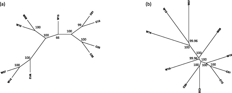
The results of the analysis of the soybean data using both SNAPP and SVDquartets are shown in Figure 8. The SNAPP analysis was run for 2.239 million iterations, corresponding to 28 days on a desktop Linux machine (2× Quad Core Xeon E5520/2.26 GHz/32 GB). There were important indications of a lack of convergence of the method, with nearly all effective sample size (ESS) values <200 and trace plots indicating issues in convergence. The full details of the analysis and assessment of convergence are described in the Supplemental Information. The SVDquartets method with 100 bootstrap samples and 20 000 quartets sampled per replicate required ∼600 h (which corresponds to 25 days) of time to complete using the same desktop Linux machine, though it was run in parallel using six processors, and thus took only 4.5 days to complete. We note that this can easily be parallelized further, with the only limits due to availability of processors.

Fig. 8.

Results of the analysis of the soybean data. (a) Tree estimated by SVDquartets with bootstrap support values. (b) Maximum clade credibility tree estimated using SNAPP

Even though we have subsampled and filtered the original dataset, our results are in agreement with the findings of the original report (Lam et al., 2010). In their analyses, they found that cultivated soybeans formed a tight subclade. Furthermore, they concluded using the Bayesian clustering program STRUCTURE and principal component analysis that C01 and C12 show a clear separation from the cultivated cluster. Also, the phylogenetic tree in Lam et al. (2010) has cultivars as part of the clade that includes wild-type soybeans W08, W10 and W15, while W07, W12 and W14 are part of another cluster. One can see that the results in Figure 8 for both trees are in general consistent with the previous findings. Of course, there are important differences between the trees as well.

5 CONCLUSION

We have presented a method to reliably infer the valid split in a set of four taxa. We have demonstrated that the method performs very well over a range of simulation conditions. The method can be easily extended for use in inferring species phylogenies in larger taxon samples, as demonstrated by our applications to the rattlesnake data and to the soybean data. The method thus makes a valuable contribution to the collection of methods for inferring species-level phylogenetic trees under the coalescent model for either multi-locus or unlinked SNP data.

REFERENCES

- Allman ES, Rhodes JA. Phylogenetic ideals and varieties for the general Markov model. Adv. Appl. Math. 2008;40 arXiv:math.AG/0410604. [Google Scholar]
- Bryant D, et al. Inferring species trees directly from biallelic genetic markers: bypassing gene trees in a full coalescent analysis. Mol. Biol. Evol. 2012;29:1917–1932. doi: 10.1093/molbev/mss086. [DOI] [PMC free article] [PubMed] [Google Scholar]
- Chifman J, Kubatko LS. Identifiability of the unrooted species tree topology under the coalescent model with time-reversible substitution processes. 2014 doi: 10.1016/j.jtbi.2015.03.006. http://arxiv.org/abs/1406.4811. [DOI] [PubMed] [Google Scholar]
- Degnan J, Salter L. Gene tree distributions under the coalescent process. Evolution. 2005;59:24–37. [PubMed] [Google Scholar]
- DeGeorgio M, Degnan J. Fast and consistent estimation of species trees using supermatrix rooted triples. Mol. Biol. Evol. 2010;27:552–569. doi: 10.1093/molbev/msp250. [DOI] [PMC free article] [PubMed] [Google Scholar]
- Eriksson N. Tree construction using singular value decompsition. In: Pachter L, Sturmfels B, editors. Algebraic Statistics for Computational Biology. 2005. Chap 19. Cambridge University Press, Cambridge, pp. 347–358. [Google Scholar]
- Golub GH, Van Loan CF. Matrix Computations. 4th edn. Baltimore, Maryland: Johns Hopkins University Press; 2013. [Google Scholar]
- Heled J, Drummond A. Bayesian inference of species trees from multi-locus data. Mol. Biol. Evol. 2010;27:570–580. doi: 10.1093/molbev/msp274. [DOI] [PMC free article] [PubMed] [Google Scholar]
- Huang H, et al. Sources of error for species-tree estimation: impact of mutational and coalescent effects on accuracy and implications for choosing among different methods. Syst. Biol. 2010;59:573–583. doi: 10.1093/sysbio/syq047. [DOI] [PubMed] [Google Scholar]
- Jukes T, Cantor C. Evolution of Protein Molecules. New York: Academic Press; 1969. pp. 21–132. [Google Scholar]
- Kingman JFC. The coalescent. Stoch. Proc. Appl. 1982a;13:235–248. [Google Scholar]
- Kingman JFC. Exchangeability and the evolution of large populations. In: Koch G, Spizzichino F, editors. Exchangeability in Probability and Statistics. Amsterdam: North-Holland Elsevier; 1982b. pp. 97–112. [Google Scholar]
- Kubatko LS, et al. STEM: species tree estimation using maximum likelihood for gene trees under the coalescent. Bioinformatics. 2009;25:971–973. doi: 10.1093/bioinformatics/btp079. [DOI] [PubMed] [Google Scholar]
- Kubatko LS, et al. Inferring species-level phylogenies and taxonomic distinctiveness using multilocus data in Sistrurus rattlesnakes. Syst. Biol. 2011;60:393–409. doi: 10.1093/sysbio/syr011. [DOI] [PubMed] [Google Scholar]
- Lam HM, et al. Resequencing of 31 wild and cultivated soybean genomes identifies patterns of genetic diversity and selection. Nat. Genet. 2010;42:1053–1059. doi: 10.1038/ng.715. [DOI] [PubMed] [Google Scholar]
- Lee TH, et al. SNPhylo: a pipeline to construct a phylogenetic tree from huge SNP data. BMC Genomics. 2014;15:162. doi: 10.1186/1471-2164-15-162. [DOI] [PMC free article] [PubMed] [Google Scholar]
- Liu L, Pearl D. Species trees from gene trees: reconstructing Bayesian posterior distributions of a species phylogeny using estimated gene tree distributions. Syst. Biol. 2007;56:504–514. doi: 10.1080/10635150701429982. [DOI] [PubMed] [Google Scholar]
- Liu L, et al. Coalescent methods for estimating phylogenetic trees. Mol. Phylogenet. Evol. 2009a;52:320–328. doi: 10.1016/j.ympev.2009.05.033. [DOI] [PubMed] [Google Scholar]
- Liu L, et al. Maximum tree: a consistent estimator of the species tree. J. Math. Biol. 2009b;60:95–106. doi: 10.1007/s00285-009-0260-0. [DOI] [PubMed] [Google Scholar]
- Liu L, et al. Estimating species phylogenies using coalescence times among sequences. Syst. Biol. 2009c;58:468–477. doi: 10.1093/sysbio/syp031. [DOI] [PubMed] [Google Scholar]
- Liu L, et al. A maximum pseudo-likelihood approach for estimating species trees under the coalescent model. BMC Evol. Biol. 2010;10:302. doi: 10.1186/1471-2148-10-302. [DOI] [PMC free article] [PubMed] [Google Scholar]
- Maddison W. Gene trees in species trees. Syst. Biol. 1997;46:523–536. [Google Scholar]
- Rambaut A, Grassly NC. Seq-Gen: an application for the Monte Carlo simulation of DNA sequence evolution along phylogenetic trees. Comput. Appl. Biosci. 1997;13:235–238. doi: 10.1093/bioinformatics/13.3.235. [DOI] [PubMed] [Google Scholar]
- Rannala B, Yang Z. Bayes estimation of species divergence times and ancestral population sizes using DNA sequences from multiple loci. Genetics. 2003;164:1645–1656. doi: 10.1093/genetics/164.4.1645. [DOI] [PMC free article] [PubMed] [Google Scholar]
- Snir S, Rao. S. Quartet MaxCut: a fast algorithm for amalgamating quartet trees. Mol. Phylogen. Evol. 2012;62:1–8. doi: 10.1016/j.ympev.2011.06.021. [DOI] [PubMed] [Google Scholar]
- Strimmer K, von Haeseler A. Quartet puzzling: a quartet maximum likelihood method for reconstructing tree topologies. Mol. Biol. Evol. 1996;13:964–969. [Google Scholar]
- Strimmer K, et al. Bayesian probabilities and quartet puzzling. Mol. Biol. Evol. 1997;14:210–213. [Google Scholar]
- Tavare S. Some probabilistic and statistical problems in the analysis of DNA sequences. Lect. Math. Life Sci. 1986;17:57–86. [Google Scholar]
- Than C, Nakhleh L. Species tree inference by minimizing deep coalescences. PLoS Comput. Biol. 2009;5:e1000501. doi: 10.1371/journal.pcbi.1000501. [DOI] [PMC free article] [PubMed] [Google Scholar]
Associated Data
This section collects any data citations, data availability statements, or supplementary materials included in this article.