Exploring the Connectome

Abstract

A system for interactively exploring petavoxel volumes from high-throughput electron microscopy data streams that supports concurrent visualization of high-resolution volumes and voxel segmentation data. The visualization-driven system design handles incomplete data and improves scalability over previous approaches. Researchers have employed the system on a 1-teravoxel mouse cortex volume.

Reconstructing the human connectome is one of the 21st century’s major scientific endeavors. By deciphering the human brain’s neural circuits, comprising billions of neurons and their interconnections (synapses), connectomics researchers hope to improve their understanding of brain function as well as pathologies such as Alzheimer’s disease and autism. However, the mammalian connectome is immensely complex, and the huge amount of imaging data that must be acquired, stored, and processed presents a big challenge for neuroscientists. For example, the C. elegans worm’s connectome, consisting of a mere 300 neurons and their 7,000 connections, took over a dozen years to complete.¹ Only recent advances in high-throughput and high-resolution microscopic imaging have made it possible to start tackling mammals.

Modern microtomes and electron microscopes (EMs) can produce volumes of scanned brain tissue in 25- to 50-nm slices with a pixel resolution of 3 to 5 nm,² as compared to 200 nm for optical microscopes. The higher resolution enables tracing of detailed neural connections at the resolution level of individual synapses, but it also makes processing and analyzing the scanned data a major bottleneck for connectomics. For example, a 1-mm³ EM volume of brain tissue would generate a 1-Pbyte volume of data, and scanning the data with a throughput of roughly 10 Mpixels per second would take several years.² Currently, high-throughput acquisition requires continuous data streaming over months or even years, which effectively implies the need for processing and visualization algorithms that can handle incomplete data—that is, data that hasn’t yet been completely scanned.

Reconstructing the synaptic connections between neurons often involves laborious manual segmentation of the scanned volume data, along with semiautomatic or fully automatic approaches.³ However, understanding the data requires interactive 3D visualization of the scanned volume, visual proofreading of the segmentation, and 3D navigation inside the volume—all within the context of large-scale EM data volumes. Preprocessing the data into a hierarchical representation— as usually happens with interactive visualization of large volumes—incurs an unacceptably long time between acquisition and visualization. Novel visualization paradigms and systems are therefore necessary to facilitate the interactive exploration and analysis of large-scale microscopy data streams.

We have developed a scalable end-to-end system design for the interactive 3D exploration and navigation of segmented high-resolution EM data.⁴ It offers a flexible volume-processing and visualization framework that handles petascale (that is, petavoxel) volume data and can deal with incomplete data. Here, we describe the two main parts of our system—a data-driven pipeline that’s triggered by the actual EM data acquisition, and a visualization- driven pipeline that’s triggered by the user interacting with the visualization. We explain how both pipelines and their modules scale to petavoxel volumes and, furthermore, illustrate the real-world use of our system for a mouse cortex volume of one teravoxel in size.

Previous Work in Connectomics Visualization.

Our system is related to a large collection of prior work; we highlight only the most important connections here. Sebastian Seung gave a good introduction to connectomics and its recent developments, including advances in high-resolution and high-throughput electron microscopy (EM) imaging.¹ Davi Bock and his colleagues showed how EM circuit reconstruction and the resulting network graph of connected neurons can help find a relationship between a brain area’s structure and function.²

The system we describe in the main article is based partly on previous research on petascale volume rendering and visualization of neuroscience datasets. Markus Hadwiger and his colleagues introduced a volume-rendering scheme for extremely large EM data, focusing on a multiresolution virtual-memory architecture and on-the-fly construction of volume blocks with a thorough performance and scalability analysis.³ Won-Ki Jeong and his colleagues described two systems for interactive exploration and analysis of EM images.⁴ They focused on manual and semiautomatic neuron tracing and on-the-fly edge detection for improved rendering of neural processes. Previously, we described a general system for rendering multiple volumes in addition to segmentation data, for neurosurgical applications.⁵ Although that system also employed out-of-core strategies, it could only handle much smaller data sizes than the system we describe in the main article.

Our visualization subsystem uses GPU volume ray casting, the most common approach for GPU volume rendering. A main constraint for GPU-based approaches is the limited GPU memory. To accommodate large volumes, Eric La Mar and his colleagues developed out-of-core and multiresolution volume-rendering approaches, often based on hierarchical octree bricking schemes.⁶ These approaches partition the data into subbricks and compute a multiresolution data hierarchy (such as an octree) during preprocessing. During rendering, only the active working set of these bricks (for example, all bricks in the view frustum) must be downloaded to the GPU, thereby alleviating GPU memory restrictions. However, all previous multiresolution volume renderers require building the multiresolution hierarchy during preprocessing, which isn’t feasible for our scenario of dynamically streaming image data.

A preprocessing step is also required by all previous systems that support volume data streaming for progressive rendering, such as the ViSUS (Visualization Streams for Ultimate Scalability) system.⁷ The GigaVoxels⁸ and CERA-TVR⁹ systems perform explicit octree traversal on the GPU by using the k-d restart algorithm. However, this requires holding the entire path from every leaf to the root in GPU memory, which can result in large numbers of updates per frame. Our system avoids many drawbacks of explicit octree traversal by using a virtual-memory approach that allows direct access to any requested resolution, without having to traverse the entire hierarchy of coarser resolution levels.³

Much research has covered volume rendering on supercomputers. ¹⁰ This is especially useful for in-situ visualization of large-scale simulations. Computing the visualization on the same machine as the data avoids the need to move large data. However, this approach isn’t feasible for microscopy data. Our data streams don’t originate from large-scale simulations, but from acquisition setups that aren’t directly connected to a supercomputer. Our system streams data to the GPU-based visualization, but only as the actual visibility requires. Researchers have applied such a display-aware approach to on-the-fly image alignment and stitching at a resolution that matches the desired output resolution.¹¹

(See the sidebar for related work in connectomics visualization.)

System Overview

Our system has two main parts (see Figure 1):

Figure 1.

System overview. Petascale volumes are acquired as a stream of image tiles from the electron microscope (EM). Each raw image tile is processed individually in the input stream. Everything else is visualization-driven. Ray casting operates in virtual volume space, detecting missing blocks for visible volume blocks that aren’t in GPU memory. Then the system constructs the missing blocks in 3D by stitching and resampling the corresponding tiles from the 2D input stream.

• The data-driven pipeline handles image acquisition, data storage, and 2D mipmap generation.

• The visualization-driven pipeline supports visualization and 3D block construction.

Data generation starts on the left side of Figure 1 and propagates to the right. In a wider sense, it includes more complex preprocessing tasks such as registration and segmentation. Most of our system is visualization-driven—that is, driven by the actual visibility of small 3D blocks on screen during ray casting (see the right side of Figure 1). We operate in virtual volume space, which is our volume’s reference space and corresponds to the 3D tissue block that the EM is imaging. During ray casting, if the renderer detects that a data block is missing, it requests that block. The system handles the request during volume construction and then downloads the newly constructed block into GPU memory.

The system’s design pays special attention to modularity for integration of future changes, such as new data modalities or novel preprocessing algorithms.

System Environment

The system environment employs a client-server network architecture (see Figure 2). Generally, we allow for a flexible setup that lets each module run on a separate machine, connected via a high-bandwidth LAN. Optionally, we can configure the system to run all modules on the same machine, omitting network communication. The visualization archive is on a shared file system, letting multiple users access the data. Rendering occurs either on a separate rendering server that sends the final images to a thin client or directly on the PC that displays the final image. All network communication is based on TCP sockets and can use image compression to reduce network bandwidth.

Figure 2.

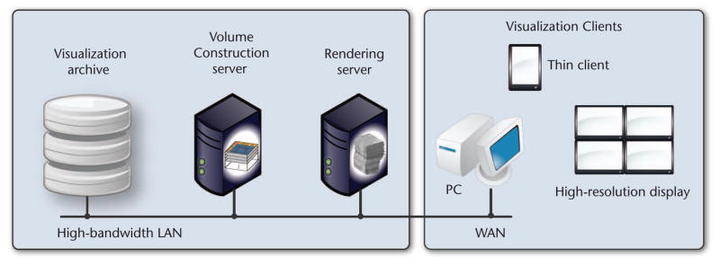
The system environment. A configurable client-server setup supports the use of separate machines for our system’s different modules.

For handling missing data, our modules are multithreaded to avoid blocking other computations or delaying rendering because of uncompleted data requests. The visualization stage runs with a rendering thread, a GUI or user input thread, and a thread for data requests to the volume construction module. Once the renderer has issued a data request, it continues rendering without waiting for the request to complete. The ray caster can deal with incomplete data by either substituting a data block with its lower-resolution version—if one is available—or skipping the block until it has been loaded.

Data-Driven Pipeline

The goal of our data-driven pipeline is to process new data as soon as the EM has scanned it and to make it available for visualization. Each system module is designed to scale to petavoxel volumes.

Acquisition

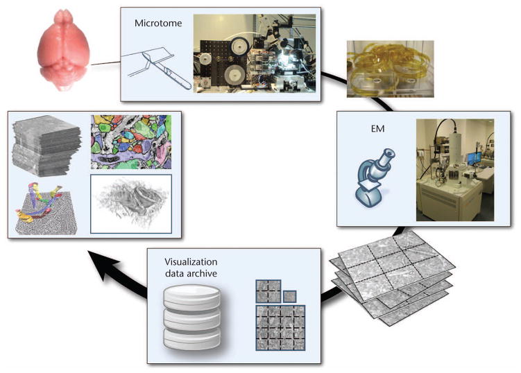
In the acquisition pipeline (see Figure 3), we first take a tiny sample of a mouse or rat brain and solidify it using an epoxy resin. We then cut the solidified sample into 25- to 50-nm slices using Harvard’s Atlum (automatic tape-collecting lathe ultramicrotome). To enhance the tissue’s contrasts, we stain it with heavy metals.

Figure 3.

The acquisition pipeline. We cut tissue samples into ultrathin slices using Harvard’s automatic tape-collecting lathe ultramicrotome (Atlum) and image them using an EM. We then store the acquired image tiles in a data archive. After 2D mipmap generation, the data can be used for different applications, such as visualization, segmentation, and fine-grained registration.

Next, we image the collected microscope tapes of tissue slices, using a scanning EM with a resolution of 3 to 5 nm. The EM acquires image tiles of a fixed pixel resolution and stores the raw data together with metadata in a central acquisition archive. The metadata includes each tile’s magnification, position, and orientation (stored in an alignment matrix) and current EM settings.

Raw-Tile Processing

This module processes tiles arriving from the EM. It polls constantly for new tiles in the acquisition archive, processes them, and stores the data in a compressed form in the visualization archive.

Figure 3 depicts raw-tile processing and the visualization archive in the context of the acquisition pipeline. Raw-tile processing comprises construction of a 2D mipmap for each tile and subdivision of each mipmap level into smaller subtiles. We chose a 128 × 128 subtile for optimized disk access and disk storage. Additionally, smaller subtiles can be handled more efficiently in the resampling phase of volume data construction, as we describe later. Subtiles can be compressed using JPEG at 2 bits per pixel (bpp) and stored in the visualization archive.

We store each mipmap level in a separate file. To improve disk access time, we store the subtiles in each file in Morton order. This approach preserves data locality and increases cache coherency. The visualization archive also allows external segmentation to access the image data and to store segmentation results and any manual data labeling.

In principle, we could use the same data archive for raw and preprocessed data. However, for organizational reasons, it’s often better to have two separate archives. The acquisition archive storing the raw microscope data is closely connected to the actual acquisition, so the EM operators can manage it directly in cooperation with the biologists. All further processing of the data for visualization (or segmentation) employs the visualization archive, which is managed by the visualization experts and biologists and stores the compressed 2D mipmaps.

Because every new tile must undergo raw-tile processing, this module must be able to handle the microscope’s sustained data rate—for example, 10 Mpixels/sec. at 8 bpp. Currently, our raw-tile processing performs at 85 Mpixels/sec.

The 2D mipmapping lets us construct the 2D mipmap of each incoming tile right away and use it immediately for visualization if it’s visible on screen. In contrast, constructing a 3D mipmap would require either waiting for all required slices from the EM before computing a 3D multiresolution hierarchy or recomputing the 3D hierarchy every time a new slice arrives.

Registration

Attached to each EM image tile is an affine alignment matrix (a transformation matrix), which corresponds to the movement of the EM’s platform stage. This matrix is stored only once for each tile and inherited by all subtiles. The alignment matrix can be iteratively refined by external registration to reflect tile alignment in both 2D and 3D. However, the registration changes no image data, and our raw-tile processing is completely independent of any registration. The registration changes only the alignment matrix. Tile stitching is performed only on demand during volume-data construction.

We can employ on-the-fly registration for dynamic EM acquisition. In many cases, the region of interest is much smaller than the entire slice of the original tissue sample. In such cases, without scanning the entire slice at the highest resolution, we can progressively scan the slice at different magnification levels by narrowing the EM’s field of view—like zooming in on a specific region. Figure 4 shows three tiles—a low-magnification image for the entire view and two higher-magnification images for the region of interest—aligned into a single coordinate system.

Figure 4.

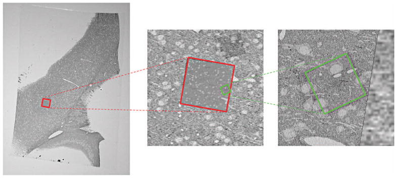
On-the-fly registration of three EM image tiles at different scales. A low-magnification image for the entire view and two higher-magnification images for the region of interest are aligned into a single coordinate system.

In this scenario, we acquire each tile at a different image scale and spatial location. To align such images, we use a fixed-size reference grid—for example, one at the screen resolution—and register two images on the grid. Because the images’ resolutions differ from the grid, we subsample or supersample each image according to the magnification level.

In our implementation, the lower-level image I_L is the background (reference) image. We rigidly transform the higher-level image I_H (for example, by rotation, translation, and scaling) to minimize the image difference energy:

$$E=\sum _{i=1}^n{\left|\right|I_L(x_i)-(T·I_H)(x_i)\left|\right|}^2,$$

where T is the rigid alignment transformation, x_i is the ith pixel index on the grid, and I(x_i) is the pixel value of I at x_i. To minimize E, we use a gradient descent that iteratively updates the transformation parameters, such as a translation vector, a rotation angle, or a zoom factor, along the negative gradient direction.

The registration can be semiautomatic if desired. As a tile enters the system from the EM, users can interactively navigate a 2D slice view to refine the registration if a misalignment is visible. The registration is implemented on the GPU, and its running time is independent of the tile size because the computation occurs on the grid. We’ve observed about 3 ms per single run of registration on a 256 × 256 grid on an Nvidia Fermi GPU (GTX 580).

Visualization-Driven Pipeline

To explain the visualization-driven pipeline’s modules, we focus first on our volume-data construction method. Next, we introduce our GPU-based volume ray-casting framework⁴ and then describe how we extended the system to segmentation data and neuronal-connectivity data based on synapses. Figure 5 shows renderings of our volume visualization system.

Figure 5.

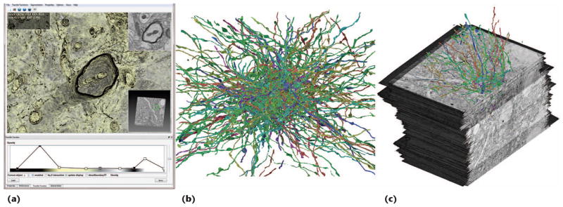
Our system supports visualization of large-scale EM volumes, their segmentation information, and synaptic connections. (a) A screenshot of our application showing an unsegmented axon. (b) Segmented axons. (c) A combined rendering of EM data with segmented axons.

Visualization-Driven Volume-Data Construction

Volume construction is driven entirely by the visualization module (see Figure 1). Data is constructed and loaded into GPU memory only if the ray caster has requested it. Volume construction is therefore independent of the data size. The ray caster issues a 3D block construction request (at a certain position and resolution level) only if the block is visible on screen and the data request can’t be fulfilled from one of the caches in the visualization module.

Our multiresolution ray casting requires construction of only the data for the requested resolution level. It uses no other resolution levels, unlike octree approaches.

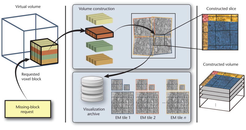
Figure 6 depicts volume construction. Once the ray caster requests a block (the bottom left of Figure 6), the system constructs the block at the requested resolution and transmits it to the visualization module. Block construction has two main parts. First, the system determines the 2D subtiles that intersect the 3D target block and fetches them at the requested resolution from the visualization archive. To efficiently retrieve the correct subtiles, we implemented a compact index structure that’s based on the Morton order of the subtiles and fits easily into main memory.

Figure 6.

Visualization-driven volume construction. The system stitches and resamples only the visible 3D blocks in the virtual multiresolution volume, computing the result at the requested resolution.

Second, the system stitches and resamples the 2D subtiles directly into the 3D target grid. Stitching is determined by each tile’s alignment matrix. We implemented fast stitching and resampling to any target resolution on the GPU, using texture mapping and fragment shaders. Because of the large slice distance and resulting anisotropy of our EM data (for example, an aspect ratio of 1:10), we can simplify 3D block construction. To do this, we allow a 3D target block to be resampled by simply stitching the image subtiles in 2D, without performing 3D filtering. Then, we store the result in the correct 3D location. For reconstruction filtering, we can use either GPU bilinear filtering or higher-order filters implemented in the fragment shader. If the EM hasn’t yet scanned the requested data, we report the block as empty and skip block construction.

Our volume construction’s modular design lets it also serve as a basis for additional computations such as automatic segmentation or data analysis. The only requirement is that the computations employ 2D or 3D blocks at a certain location with a certain resolution.

Volume Rendering

Our volume rendering differs from that of previous systems in three ways. First, our ray caster doesn’t create and traverse a tree structure, such as an octree or k-d tree. Instead, it employs a multilevel, multiresolution virtual-memory architecture that scales well to extremely large volumes. This design is more efficient for deep-resolution hierarchies because it requires no tree traversal and no need to maintain a tree structure.

Second, our volume rendering reduces latency by allowing each sample to be fetched directly from any resolution level and enabling switching between resolutions without constructing intermediate lower resolutions.

Finally, it supports arbitrary downsampling ratios between resolution levels, which enables better accommodation of anisotropic voxel data.

The virtual-memory architecture

We operate in the virtual-volume reference space and start by subdividing the volume into small 3D blocks. We use 32³ blocks and add a single voxel boundary for correct interpolation between neighboring blocks. Only the working set of these currently required (visible) blocks resides in GPU memory, in a large 3D cache texture that’s updated dynamically.

To access a sample in the original volume, we must translate the sample’s position to a coordinate in cache texture space, which takes place on the fly using page-table lookups. The original volume therefore becomes a virtual volume that’s accessed via a page table; only the smaller cache texture and the page table must be stored on the GPU. If a block doesn’t reside in the cache texture, it’s flagged as unmapped (missing) in the page table.

However, one indirection layer (page table) is insufficient for very large volumes. Our system can therefore virtualize not only the original volume but also page tables. We refer to the top-level page table in the resulting hierarchy as the page directory. Currently, we use two indirection layers, which already enables scalability to several hundred teravoxels.⁴ This contrasts with octree approaches, which require traversing many more levels.

For multiresolution rendering, we conceptually have a separate hierarchy of page tables for each data resolution level. However, because the blocks of different resolution levels have the same voxel size (for example, 32³), we can map blocks of any resolution level into the same 3D cache texture. The only structure that directly reflects the data’s multiresolution nature is the multiresolution page directory.

Ray casting virtual multiresolution volumes

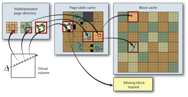
Ray casting marches along the ray from sample to sample, performing hierarchical address translation for each one to map the virtual-volume position to the corresponding position in the 3D cache texture (see Figure 7). A sample’s position on the ray is given by a normalized coordinate in virtual volume space. At each sample point, we compute the desired level of detail (LOD) for accessing the corresponding data resolution level. We estimate the LOD by computing the size of the current voxel’s projected screen space. We use the sample’s position and LOD for the address translation lookup in the corresponding level of the multiresolution page directory.

Figure 7.

Ray casting occurs in a virtual multiresolution volume, in which a hierarchy of page tables represents each resolution. Ray casting accesses the actual volume data by performing on-the-fly address translation to access blocks in virtual memory. If a data block is missing, the ray caster generates a request for that block and propagates the request to the visualization-driven volume construction.

Many successive samples along a ray will map to the same page directory and page table entries. So, we can significantly reduce the texture lookup overhead by exploiting spatial coherence and reducing the number of required texture fetches. The closer a page table entry is to the hierarchy’s root (the page directory), the less frequently it must be fetched. For example, with 32³ blocks, the page table is accessed only every 32 voxels for an axis-aligned ray, and the page directory is accessed only every 1,024 voxels.

During ray casting, the system detects missing data whenever a page directory or page table entry is accessed that doesn’t point to data but is flagged as unmapped. This generates a request for the missing 3D block of visible data. This request propagates backward in the pipeline. If none of the system’s caches (in GPU or CPU memory or in the volume construction module) can meet it, the request triggers the visualization-driven construction of volume data from 2D image tiles. To ensure interactive frame rates, we limit how many blocks can be downloaded to the GPU each frame. Furthermore, to decide which blocks are no longer needed and can be swapped out of the cache and discarded, we employ an LRU (least recently used) scheme and track block usage in the ray caster.

For further optimization, we implemented empty-space skipping on the granularity level of page table entries. If a data block is reported empty, it’s not downloaded to the GPU, and its page table entry is flagged as empty. Our system performs empty-space skipping by culling against the current transfer function.

Segmented Data and Synapse Identification

Segmentation is crucial in connectomics research. Scientists use it to partition data into neuronal structures such as axons and dendrites, to trace structures connected by synapses, and to determine their spatial relationships. (An axon is a long, narrow, tubular structure that conducts electrical impulses away from a neuron’s cell body. These impulses pass over a synapse to a dendrite, a treelike extension of another neuron.) To this end, our system supports the visualization of sparse segmentations (in which only selected structures are traced), dense segmentations (in which all structures are traced), and labeled synapses.

Visualizing segmented data

A detailed description of our system’s segmentation modules and tools is outside this article’s scope, and we treat the segmentation algorithms as black boxes. However, we assume that the segmentation runs on image data from the visualization archive and that the same archive stores the final segmentation results.

We store segmentation data as image data slices (like the original EM data), in which each pixel contains the ID of the labeled object it belongs to. To allow for a large number of distinct objects, we store these IDs as 24-bit data, which lets us store over 16 million objects. Once the segmentation data arrives at the visualization archive, we compute 2D mipmaps for each slice, just as we described earlier for the EM data. The main difference is that we must use a different downsampling filter because the segmentation data comprises object IDs that must not be interpolated. The straightforward choice for downsampling is nearest-neighbor filtering, but we could use more elaborate downsampling algorithms, such as a rank filter.

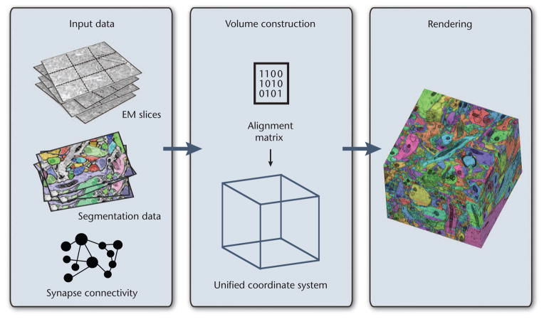
Figure 8 shows the main steps of our visualization scheme for segmented data. For highest possible generality, we handle the segmentation volume as an additional data volume and perform multivolume rendering. This lets us easily extend our system to include additional data volumes, such as functional brain data. To handle two volumes, we run two instances of the volume construction module and two instances of the virtual-memory architecture. We allocate separate cache textures for the EM and segmentation data because they’re usually of different types—that is, 8-bit intensity values for EM data and 24-bit integer IDs for segmentation data.

Figure 8.

Multivolume visualization. All input data is stored in the visualization archive. Data requests construct 3D blocks for all requested volumes in a unified coordinate system (the virtual volume). During ray casting, multiple volumes can be sampled and combined into the final rendering.

Eventually, the ray caster samples and renders the original data simultaneously with the segmentation data. Our system supports different rendering modes, using the current sample’s object ID to assign and modify certain properties, such as color and opacity. The ray caster then blends these properties with the original EM data.

Synapse labeling

The system can render labeled synapses that are stored in tabular format in the visualization archive. Each table entry defines a single synapse consisting of its virtual volume position, a text label, the IDs of the two objects it connects (one axon and one dendrite), and some additional meta-information.

During rendering we can display all loaded synapses, their labels, and their connections. Additionally, users can add synapses to the data, which the system then stores in the visualization archive. Synapses are rendered as small geometric shapes, located at the position specified in the synapse table. To simplify navigation in the volume, users can select individual synapses, which are then automatically centered in the current view. The right image in Figure 9 shows a volume rendering of segmented axons, with a close-up of a labeled synapse.

Figure 9.

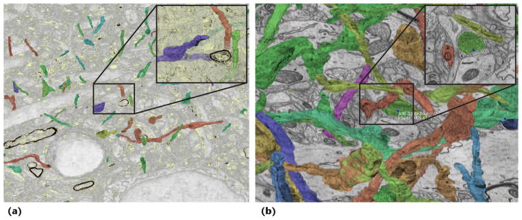
Volume-rendering segmentation data and synapse labeling. The left and middle images show different zoom factors and transfer functions for volume-rendering segmentation data. The transparent transfer function in the middle image lets users visually follow otherwise occluded structures. The right image shows a labeled synapse in 3D and slice views. Users can automatically navigate to and zoom in on a synapse by selecting it in the 3D view. The view parameters and clipping planes adjust automatically.

Results on a Mouse Cortex

Our collaborating neuroscientists are working on the segmentation and analysis of a mouse cortex EM dataset with a resolution of 21,924 × 25,790 × 1,850 voxels, which is roughly 1 Tvoxel. Over several months, the scientists have segmented several hundred structures (mostly axons) by manually tracing them from slice to slice.

In our dataset, we have segmented 329 axons and 4 dendrites, and each dendrite makes many synapses. Most segmented axons are oriented along the z direction, spanning 490 dataset slices on average. Approximately a dozen axons span the entire 1,850 slices; the smallest axons span only two slices.

In our dataset, a segmented axon consists of over 6.2 million voxels on average, with a minimum of 12 voxels and a maximum of 37.5 million voxels. The segmented axons constitute less than 0.2 percent of the dataset. We have detailed information on 263 synapses, including their location, label, and IDs of the axon and dendrite that each synapse connects. Each segmented dendrite is connected to 53 labeled synapses on average, with a minimum of one synapse and a maximum of 101 synapses. Axons, on the other hand, average only two labeled synapses, with a minimum of one and a maximum of seven.

Figures 5 and 9 show different renderings of this dataset, including the segmented axons and labeled synapses.

Performance

We tested our system on three 12-core dual-CPU 3-GHz machines, each with 48 Gbytes of CPU RAM and an Nvidia Quadro 6000 GPU with 6 Gbytes of GPU RAM. We implemented the system in C++, the ray caster in GLSL (OpenGL Shading Language), and the tile processing in CUDA (Compute Unified Device Architecture) and OpenMP.

Currently, the three machines run, respectively, the raw tile processing, the volume construction, and the visualization module, including the user interface. This setup lets us exploit parallelism between the different modules and maximize the available cache sizes. All network communication uses TCP/IP and Windows Sockets 2 over a 1-Gbyte network.

Table 1 shows the timing results for raw-tile processing and 3D-block construction (registration, stitching, and resampling), as well as the frame rates for ray-casting the 1-Tvoxel dataset, including segmented volume rendering. We used two transfer functions to measure ray casting. The first was a linear ramp; the second was a more transparent transfer function that lets us see farther inside the volume (see the middle image of Figure 9).

Table 1.

Our system’s performance. We measure volume rendering for a 1,024 × 768 pixel viewport.

Module	Performance
Raw-tile processing	85 Mpixels/sec. for 8-bit pixel data
Registration	20 Mpixels/sec. output
Stitching and resampling	30–65 Mpixels/sec. output
Volume rendering of EM data*	75 fps for transfer function 1 12 fps for transfer function 2
Volume rendering of segmented data*	70 fps for transfer function 1 9 fps for transfer function 2

^*Transfer function 1 was a linear ramp for color and opacity; transfer function 2 was a more transparent transfer function.

The raw-tile processing clearly meets the requirement of 10 Mpixels/sec., given by the microscope’s current data acquisition rate. Volume rendering, based on our multiresolution virtual-memory architecture, achieves interactive frame rates for concurrent rendering of both the original and the segmentation volume.

Scalability

Our system achieves its scalability primarily in its volume representation (including multivolumes), volume traversal, and ray casting.

Volume representation

Our virtual multiresolution volume representation is extremely scalable because of the small number of levels needed for the page table hierarchy. Two or three levels are sufficient for extremely large volumes, resulting in easily manageable page directory sizes.⁴ Our current implementation uses two levels (with 32³ voxel blocks), which, for example, allows rendering a 4-Tvoxel volume with a page directory of only 32 × 32 × 4. This makes it easy to accommodate multiple volumes and handle multiple page directories as well as their corresponding page-table hierarchy. A page-table hierarchy with three levels and page directory sizes under 643 could represent even a dataset of several hundred petavoxels.⁴

Volume traversal

In our system, volume traversal is extremely efficient. To access an arbitrary resolution level, we only have to traverse the very compact page-table hierarchy (that is, two or three levels), effectively resulting in an (1) traversal time for accessing any resolution level. In contrast, octree-based schemes must traverse the tree from the root to the requested resolution level, which is logarithmic in the number of octree voxels. These differences show up clearly in practice, especially in a typical neuroscience use case involving the inspection of data in high resolution. We illustrated this in a more detailed scalability analysis.⁴

Ray casting

For rendering segmented and multiple volumes, we have a separate page-table hierarchy for every volume. This lets us store sparse segmentation data in a cache smaller than one for dense EM data. To reduce the number of textures and texture fetches, multiple volumes can share page directory and page-table lookups. However, this requires all cache textures to have the same size and layout, which can lead to inefficient cache usage.

Our system assumes that the current working set (that is, all visible data of the desired resolution) fits into the block cache in GPU memory. If that isn’t so, the system can lower the requested resolution. Another option would be to perform multiple rendering passes on a single GPU⁵ or perform parallel rendering on multiple GPUs.

Latency

Our system’s main objective is to enable exploration of petascale EM volumes in 3D at interactive frame rates. Its design lets us completely decouple the frame rate from the time to construct missing data and download it into the GPU cache textures. So, our rendering system never stalls because of waiting for new data.

Naturally, this approach incurs a latency until all visible data have arrived at the requested resolution and a complete image is on screen. This is similar to the latency in Google Maps, but with 3D data blocks instead of 2D map tiles. The overall latency varies significantly. It ultimately depends on the number of new 3D blocks that must be constructed for a new frame in addition to already cached data. However, in typical scenarios, that number is often small, leading to low latencies.

Our system’s major design choices are the visualizaton- driven volume data construction and the multiresolution virtual memory scheme. This makes our approach scalable and allows handling multiple petavoxel volumes concurrently. In future work, we plan to develop intuitive 3D navigation metaphors for large-scale volume data. We also want to extend our system to support distributed volume rendering, especially for multiple volumes that are too large to handle efficiently with a single GPU and out-of-core memory.

Biographies

Johanna Beyer is a postdoctoral fellow at the Geometric Modeling and Scientific Visualization Center at King Abdullah University of Science and Technology. Her research interests include large-data visualization, parallel visualization, and GPU-based volume rendering for neuroscience and neurobiology. Beyer received a PhD in computer science from the Vienna University of Technology. Contact her at johanna.m.beyer@gmail.com.

Markus Hadwiger is an assistant professor of computer science at King Abdullah University of Science and Technology. His research interests are petascale visual computing, scientific visualization, volume rendering, and general GPU techniques. Hadwiger received a PhD in computer science from the Vienna University of Technology. He’s a coauthor of Real-Time Volume Graphics (AK Peters, 2006). Contact him at markus.hadwiger@kaust.edu.sa.

Ali Al-Awami is a PhD student in computer science at King Abdullah University of Science and Technology (KAUST). His research interests are scientific visualization and data navigation and exploration. Al-Awami received an MS in computer science from KAUST. Contact him at ali.awami@kaust.edu.sa.

Won-Ki Jeong is an assistant professor at the Ulsan National Institute of Science and Technology. His research interests include image processing, scientific visualization, and general-purpose GPU computing in biomedical image analysis. Jeong received a PhD in computer science from the University of Utah. He’s a member of ACM. Contact him at wkjeong@unist.ac.kr.

Narayanan Kasthuri is a postdoctoral fellow in Harvard University’s Lichtman Lab. His research interests include connectomics and neural development. Kasthuri received a D.Phil. in neurophysiology from Oxford University. Contact him at bobby.kasthuri@gmail.com.

Jeff W. Lichtman is the Jeremy R. Knowles Professor of Molecular and Cellular Biology and the Ramon Y. Cajal Professor of Arts and Sciences at Harvard University. His research interests include developmental neurobiology, where he developed methods for in vivo imaging of synapses, labeling of nerve cells with different colors, and high-resolution mapping of neural connections. Lichtman received an MD and a PhD in neurophysiology from Washington University in St. Louis. Contact him at jeff@mcb.harvard.edu.

Hanspeter Pfister is the An Wang Professor of Computer Science in Harvard University’s School of Engineering and Applied Sciences. His research interests are at the intersection of visualization, computer graphics, and computer vision. Pfister received a PhD in computer science from Stony Brook University. He’s a senior member of the IEEE Computer Society and member of ACM, ACM Siggraph, and Eurographics. Contact him at pfister@seas.harvard.edu.

References

- 1.Seung S. Connectome: How the Brain’s Wiring Makes Us Who We Are. Houghton Mifflin Harcourt; 2012. [Google Scholar]
- 2.Bock D, et al. Network Anatomy and In Vivo Physiology of Visual Cortical Neurons. Nature. 2011;471(7337):177–182. doi: 10.1038/nature09802. [DOI] [PMC free article] [PubMed] [Google Scholar]
- 3.Hadwiger M, et al. Interactive Volume Exploration of Petascale Microscopy Data Streams Using a Visualization-Driven Virtual Memory Approach. IEEE Trans Visualization and Computer Graphics. 2012;18(12):2285–2294. doi: 10.1109/TVCG.2012.240. [DOI] [PubMed] [Google Scholar]
- 4.Jeong WK, et al. Ssecrett and Neurotrace: Interactive Visualization and Analysis Tools for Large-Scale Neuroscience Datasets. IEEE Computer Graphics and Applications. 2010;30(3):58–70. doi: 10.1109/MCG.2010.56. [DOI] [PMC free article] [PubMed] [Google Scholar]
- 5.Beyer J, et al. High-Quality Multimodal Volume Rendering for Preoperative Planning of Neurosurgical Interventions. IEEE Trans Visualization and Computer Graphics. 2007;13(6):1696–1703. doi: 10.1109/TVCG.2007.70560. [DOI] [PubMed] [Google Scholar]
- 6.LaMar E, Hamann B, Joy K. Multiresolution Techniques for Interactive Texture-Based Volume Visualization. Proc. 10th IEEE Visualization Conf; IEEE CS; 1999. pp. 355–362. (VIS 99) [Google Scholar]
- 7.Summa B, et al. Interactive Editing of Massive Imagery Made Simple: Turning Atlanta into Atlantis. ACM Trans Graphics. 2011;30(2):article 7. [Google Scholar]
- 8.Crassin C, et al. GigaVoxels: Ray-Guided Streaming for Efficient and Detailed Voxel Rendering. Proc. 2009 Symp. Interactive 3D Graphics and Games; ACM; 2009. pp. 15–22. (I3D 09) [Google Scholar]
- 9.Engel K. CERA-TVR: A Framework for Interactive High-Quality Teravoxel Volume Visualization on Standard PCs. Proc. 2011 IEEE Symp. Large-Data Analysis and Visualization; IEEE; 2011. pp. 123–124. (LDAC 11) [Google Scholar]
- 10.Childs H, Duchaineau M, Ma K-L. A Scalable, Hybrid Scheme for Volume Rendering Massive Datasets. Proc. Eurographics Symp. Parallel Graphics and Visualization; Eurographics Assoc; 2006. pp. 153–162. [Google Scholar]
- 11.Jeong WK, et al. Interactive Histology of Large-Scale Biomedical Image Stacks. IEEE Trans Visualization and Computer Graphics. 2010;16(6):1386–1395. doi: 10.1109/TVCG.2010.168. [DOI] [PubMed] [Google Scholar]