Electroosmotic Flow Reversal Outside Glass Nanopores

Abstract

We report observations of a striking reversal in the direction of electroosmotic flow (EOF) outside a conical glass nanopore as a function of salt concentration. At high ionic strengths (>100 mM), we observe EOF in the expected direction as predicted by classical electrokinetic theory, while at low salt concentrations (<1 mM) the direction of the flow is reversed. The critical crossover salt concentration depends on the pore diameter. Finite-element simulations indicate a competition between the EOF generated from the inner and outer walls of the pore, which drives flows in opposite directions. We have developed a simple analytical model which reveals that, as the salt concentration is reduced, the flow rates inside the pore are geometrically constrained, whereas there is no such limit for flows outside the pore. This model captures all of the essential physics of the system and explains the observed data, highlighting the key role the external environment plays in determining the overall electroosmotic behavior.

The field of nanopore technology is rapidly approaching maturity; both natural and artifical nanopores are now regularly used for single-molecule sensing and interrogation, in diverse experiments ranging from molecular sizing and identification^1,2 to single-molecule force spectroscopy.^3,4 In nanopores with openings larger than a few nanometres, hydrodynamic effects play an important role in transport: this is well-illustrated in the behavior of natural aquaporins^5,6 and their corresponding biomimetic counterpart, carbon nanotubes.⁷ However, hydrodynamic interactions are also important when surface forces are significant, as is the case in small hydrophilic nanopores, especially if the source of the flow is a surface-governed effect such as electroosmosis.⁸

A charged object immersed in a salt solution is screened by a layer of oppositely charged counterions. The typical thickness of this electric double layer is quantified by the Debye length, which has a value of around 3 nm at 10 mM KCl, and reduces with increasing salt concentration. Within this layer there is a net charge density; the application of a tangential electric field results in the motion of these charges, which transmit their momentum to the rest of the fluid via viscous coupling. The resulting electrically driven fluid motion is called electroosmotic flow (EOF). Electroosmosis is an indispensible component in today’s microfluidic technology, not only due to its highly efficient pumping mechanism, but also in its use in more creative applications such as particle sorting,⁹ mixing,¹⁰ and microfluidic field-effect transistors.¹¹ Within nanopores, electroosmosis was shown to be the major contributor to the drag force experienced by DNA molecules undergoing voltage-driven translocation,¹²⁻¹⁴ and electroosmotic coupling between multiple DNA molecules can even reduce the electrophoretic force experienced by an individual molecule.¹⁵ Electroosmosis can also enhance the capture rate of translocating polymers.¹⁶ A complete understanding of EOF in nanopores, therefore, holds the promise for greater control over the translocation process.

In a recent Letter,¹⁷ we reported the generation of large-scale electrokinetically driven flows from a conical glass nanopore ∼150 nm in diameter. In the far field (several micrometers from the pore), we found that the flow behaves like one generated by the application of a point force P to a quiescent fluid, which results in a submerged jet of nanometric proportions; specifically, it is well-described by the Stokeslet limit of the classical Landau–Squire solution.¹⁸ The self-similar nature of the solution means that only one characteristic parameter P is required to describe the flow fully. Here we elucidate the mechanisms which result in the flow by testing how P varies under different conditions.

Our main experimental setup is an optical trap shown schematically in Figure 1; a complete description of the setup has been previously presented in the literature.^19,20 We use conical nanopores based on glass nanocapillaries. Conical nanopores are currently under investigation by many groups and have applications in DNA sensing,²¹ scanning conductance microscopy,²² and ionic current rectification.^23,24 Our pores are fabricated by pulling glass capillaries in a programmable laser puller. This results in pores with tunable sizes; in our experiments we use three different nanopore diameters: 1000, 150, and 15 nm. The capillaries are assembled into a sample cell where they connect two reservoirs filled with KCl solution of varying concentrations, buffered by Tris-EDTA at pH 8 (Figure 1A). Ag/AgCl electrodes are introduced, with the reference electrode setting the potential inside the pore, and the ground electrode located in the reservoir outside. The sample cell is placed onto an optical tweezers setup (Figure 1B). We use a single-beam gradient trap which is able to trap and manipulate small μm-sized polystyrene beads and measure forces on these with sub-pN resolution at a bandwidth of a few kHz. The particle is placed at a fixed location outside the pore. When a voltage is applied, the resulting flow field exerts a viscous force on the particle given by the Stokes equation F = 6πμRv, where μ is the viscosity, R the bead radius, and v the average fluid velocity. Measurement of this force therefore allows us to determine the local fluid velocity at that position. By moving the bead to different locations, a map of the velocity field can be created (Figure 1C). Using the properties of the Landau–Squire solution we can extract P, the characteristic force associated with the flow field (as discussed in Materials and Methods). The Landau–Squire nature of the flow can be verified more rigorously on a separate setup, where the reservoir is seeded with fluorescent particles. Particle image velocimetry measurements result in streamlines which show the shape of the flow clearly (Figure 1D).

Figure 1.

Experimental setup for measuring a Landau–Squire flow. (A) A schematic of the sample cell made from PDMS which consists of a glass nanocapillary joining two reservoirs. The cell is sealed using a glass coverslip. (B) Using optical tweezers, a polystyrene bead is positioned close to the pore opening. An applied voltage generates electrokinetic flows which exert a force on the bead. (C) By moving the bead to different locations in the x–y plane, a force map can be generated; this can be converted to a velocity map using the Stokes formula. The flow field obeys the classical Landau–Squire solution, which is characterized by a parameter P representing the force required to set up the flow. Data from the flow map can be used to extract this number. (D) Particle image velocimetry measurements provide a more rigorous test of the Landau–Squire scaling as well as high-resolution velocity maps. Scale bars in the insets are 5 μm.

We measured how P varies as a function of salt concentration. Typical results for 1000 and 150 nm pores are shown in Figure 2A and B (15 nm pore results are shown in Supplementary Figure S1) where P is plotted against the salt concentration. There are four major effects to observe here. If we consider an applied voltage of +1 V inside the pore, the first effect is that, as the salt concentration is lowered, the magnitude of P increases. Second, at some critical salt concentration, the sign of P switches dramatically, from a positive to a negative value. This indicates a reversal of direction in the large-scale flow field. Third, by comparing the data for the 1000 and 150 nm pores, we find that the critical salt concentration shifts to higher values for a smaller pore (compare with Supplementary Figure S1). Finally, the magnitude of P is asymmetric with respect to voltage reversal; the two branches corresponding to positive and negative applied voltages are not mirror images of each other. Although the negative branch exhibits similar features (increase in magnitude of P at low salt, directional switching, and pore-size dependence) as the positive branch, the magnitude of P at a given salt concentration is different between the two branches.

Figure 2.

Flow reversal as a function of salt concentration. (A) Experimentally measured values of P for applied voltages of +1 V (blue squares) and −1 V (red triangles) in a 1000 nm pore, as a function of salt concentration. As salt is reduced, P initially increases before dramatically reversing direction at a critical salt concentration. (B) In a 150 nm pore, the same behavior is observed, but with the crossover happening at a higher salt concentration. In both cases, there is an asymmetry in P with respect to voltage reversal. In all experiments, measurements were made with the bead positioned between 3 and 5 μm from the pore. (C) A cartoon summarizing the experimental results. (D) Finite-element simulations are able to reproduce the behavior for a 150 nm pore, exhibiting both flow reversal and flow rectification asymmetry. Results are also in agreement for the 15 and 1000 nm pores (Supplementary Figure S1).

The explanation of some features is straightforward. The increase in magnitude of P with decreasing salt concentration is a well-understood effect, due to the increase in the ζ-potential of glass surfaces as salt concentration is reduced.²⁵⁻²⁸ The striking asymmetry with respect to voltage reversal is an effect previously observed as “flow rectification”.¹⁷ The new phenomenon discovered in this paper concerns the dramatic switch in flow direction as a function of salt concentration and pore size that we call “flow reversal”.

In order to explain flow reversal, we first consider the expected flow direction. The pores are made from quartz (15, 150 nm) or borosilicate (1000 nm) capillaries, and at pH 8 they take on a negative surface charge due to the dissociation of silanol groups.²⁷ Therefore, under our experimental conditions, the electric double layer will contain predominantly K⁺ ions. When a positive voltage is applied inside the pore, the K⁺ ions will migrate down the cone and out the pore, resulting in an outflow, and vice versa for negative voltages. The flow behavior as dominated by the flow into and out of the tip of the pore is observed at higher salt concentrations (e.g., Figure 2A at 100 mM).

In contrast, we see that at the lowest salt concentrations the flow measured with the optically trapped particle points in the opposite direction; i.e., the flow is apparently directed outward for negative voltage and inward for the opposite polarity (Figure 2C). To investigate the origin of the anomalous behavior at low salt, finite-element simulations were carried out using the COMSOL Multiphysics package. Full details can be found in Supporting Information S2. In brief, we modeled the nanopore using a 2D-axisymmetric geometry within a box size of several micrometers. The electric potential ϕ(r) is related to the charge density ρ_e(r) = N_Ae(c_K⁺ – c_Cl^–) via Poisson’s equation

1

where e ∼ 1.6 × 10^–19 C is the elementary charge, N_A ∼ 6 × 10²³ mol^–1 is Avogadro’s constant, ε₀ ∼ 8.85 × 10^–12 F/m is the permittivity of free space, ε_r is the material-dependent relative permittivity, and c_i are the molar concentrations of each ionic species. The flux of each ionic species J_i is given by the Nernst–Planck equation

2

where D_i and z_i are the diffusion constant and valency of species i, R = 8.3145 J K^–1 mol^–1 is the molar gas constant, T the absolute temperature, and u is the velocity field. This velocity field is related to the electric body force ρ_e∇ϕ(r) and pressure gradient ∇p by the Stokes equation:

3

This coupled set of Poisson–Nernst–Planck–Stokes equations was solved to determine the steady-state concentration and velocity profiles, using a fixed surface charge density²⁷ of −0.02 C/m², relative permittivities of ε_r = 4.2 for glass and ε_r = 80 for water, and diffusion constants of 2 × 10^–9 m²/s for both K⁺ and Cl^–.²⁹ In order to compare with experiments, the quantity P was extracted for each simulation run by measuring far field fluid velocities and applying the Landau–Squire scaling (see Materials and Methods).

The simulations are able to reproduce the qualitative behavior of P for all pore sizes considered, both in terms of flow reversal and the asymmetry associated with flow rectification (the complete data are shown in Supplementary Figure S1). The results for the 150 nm pore are shown in Figure 2D. Quantitatively, the results agree to better than an order-of-magnitude, although the simulations show P increasing rapidly at low salt concentrations, whereas in experiments the trend is slower. The likely origin for this can be attributed to our assumption of fixed surface charge in the simulations, while in reality at low salt the surface charge tends to be reduced.^26,30

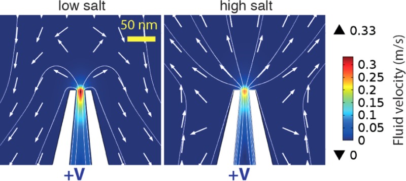
The phenomenon of flow reversal is best understood by investigating the flow patterns both in the far and near fields. Figure 3 shows flow fields at low and high salt, for a 15 nm pore. In the far field (top), the flow looks approximately Landau–Squire (Figure 3A and B). However, in the near field (bottom), there is a complex pattern directly indicative of flow reversal (C and D). At both low and high salt concentrations, the electroosmotic flow inside the pore is directed outward, as expected. However, in the low salt regime, the simulations indicate a stagnation point located outside of the pore, and most importantly, the flow profile in the far field is in the opposite direction to that inside the pore. Since this reversal takes place within a few hundred nanometers of the pore, it is not experimentally observable with the optical tweezers approach. We would like to emphasize that the flows inside the pore behave as expected under all salt concentrations, for both positive and negative voltages (Supplementary S3).

Figure 3.

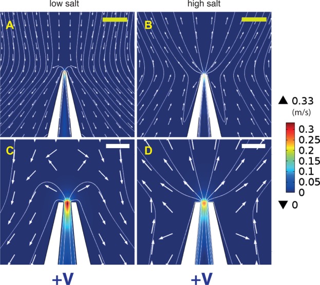
Flow patterns from finite-element simulations for a 15 nm diameter pore, with an applied voltage of +1 V. Low salt corresponds to 10 mM and high salt to 100 mM. In the far field, the flow looks approximately Landau–Squire, both at low (A) and high (B) salt concentrations. However, in the near field, a reversal behavior is observed. (C) At low salt, the flow inside the pore is directed outward, but the flow in the far field is directed in the opposite direction. (D) At high salt, both the inner as well as the far field flow are directed away from the pore. Yellow scale bars correspond to 200 nm and white scale bars to 50 nm. The arrows indicate flow direction but are normalized to have equal magnitude.

In the following section we will explain what gives rise to flow reversal in the far field at low salt concentration. Recent studies have found that it is not only the internal environment of nanopores which governs their transport properties: electric fields and surface charge external to the pore also play a significant role in determining the overall electrical conductance of the pore.^23,31 These effects are enhanced when the ratio of surface to bulk conductivity (as quantified by the Dukhin number) is high.^32,33 This corresponds to low salt concentrations and pores with a small geometrical aspect ratio (i.e., small cross-section relative to length). Because of the intricate coupling between electric and hydrodynamic flow fields, a similar sensitivity to the external environment can reasonably be expected for electroosmotic flows as well.

Since our glass pores are negatively charged and there is a finite electric field along the outer surface (see Supplementary Figure S4), an additional EOF generated from the outer walls can make a significant contribution. This can be easily shown by running the simulations with zero charge on the outer walls; in this case, no flow reversal was observed throughout the entire salt concentration range (Supplementary Figure S5). Although our simulations yield the correct result, we have additionally developed a simplified analytical model that captures the fundamental physics of the process.

As mentioned before, the electric field outside a conical nanopore behaves as if it was emanating from a point charge (Supplementary Figure S4) and points in the opposite direction to the electric field inside. Due to the small taper angles associated with the conical shape of the pores, we use an infinite cylinder for our analytical approach. We model the electric field +E_z inside and −αE_z outside (Figure 4A), where α is a parameter characterizing the relative strengths of the two electric fields. In the real system α ≈ 0.1 (Supplementary Figure S4), and we use this value in our subsequent calculations. For an infinite cylinder, analytic velocity profiles for electroosmotic flow can be calculated within the Debye–Hückel approximation²⁸ (Materials and Methods): inside the cylinder, the velocity is given by

4

and outside, by

5

where a and b are the inner and outer cylinder radii, σ the surface charge density, r the radial coordinate, and κ the inverse Debye length, which can be thought of as a parameter characterizing the salt concentration (i.e., higher values of κ correspond to higher salt concentrations). I_n and K_n are nth-order modified Bessel functions of the first and second kinds, respectively.

Figure 4.

An analytic model which captures the relevant physics. (A) The simplest model is an infinite cylinder with external and internal axially directed electric fields in opposite directions. This drives electroosmotic flows in opposite directions. The electric field ratio α was set to 0.1 in all of the analytic calculations. (B) The flow profiles inside and outside a cylinder of radius a and wall thickness a, at two different salt concentrations κ = 0.001 (solid lines) and κ = 1.0 (dashed lines), where κ is measured in units of a^–1. The maximum velocity v_max in each case was calculated at r = 0 for the inner flow and at r = λ_D for the outer flow. In the high salt case v_max,in > v_max,out, whereas in the low salt case it is the other way around. (C) The normalized momentum flux generated by the inner (solid line) and outer (dashed line) walls, as a function of salt concentration for an infinite cylinder. As salt is reduced, the inner flux saturates, while the outer flux carries on growing. (D) The normalized net momentum flux exhibits the same qualitative flow reversal behavior as observed in the experiments and simulations.

The shapes of these velocity profiles are shown in Figure 4B. As the distance from the surface is increased, the velocity profile grows over a characteristic length scale given by the Debye length λ_D = κ^–1, before eventually saturating at the Helmholtz–Smoluchowski limit v_HS = ε₀ε_rζE_z/μ ∝ σλ_DE_z/μ.

As the salt concentration is reduced, λ_D increases, and v_HS increases. However, when the Debye length becomes of the order of the cylinder cross-section, this saturation is not achieved inside the pore, and the velocity is geometrically constrained to a maximum value smaller than v_HS:

6

Such a constraint is not present on the outside of the cylinder:

7

So, as the salt concentration is further reduced, the inner velocity reaches a constant maximum value, while the outside velocity carries on increasing. This is the essential result of our analytical model. Figure 4B shows the velocity profiles at two different salt concentrations: at κ = 1.0 (in units of a^–1), the inner velocity is much larger than the outer velocity; reducing κ to 0.001 allows the maximum magnitude of the outer velocity to increase beyond that of the inner velocity, which has hardly changed.

In order to relate the analytic model to our observations, it is not velocities but momentum fluxes which should be calculated: for a given force on the fluid, the momentum delivered will in general depend on the geometry of the system. Specifically, the total momentum flux through a cross-section of fluid of area A is ρ∫_A v² dA. The computed flux, therefore, depends on the area of integration. The flux from the inside the cylinder is easily calculated; the integration area is just the area of the cylinder. However, the effective integration area outside the cylinder is infinite, and carrying out this integral for the velocity given in eq 5 leads to infinite fluxes. In reality infinite flux is prevented as the velocity decays at large distances due to pressure and inertia. But this mathematical divergence already demonstrates an important physical concept: very small outer velocities can lead to very large momentum fluxes, due to the geometry of the reservoir. It is important to note that it is not necessary for the magnitude of velocities on the outside to exceed those on the inside for the outer flux to be greater than the inner momentum flux.

Our flux argument can be formalized by choosing the integration limit to be the Debye length, bearing in mind that in reality the outer momentum flux will be larger due to entrainment. The results of calculating the fluxes from the velocity profiles given in eqs 4 and 5 are shown in Figure 4C, as a function of the nondimensional salt concentration κa. It is immediately clear that as κa is reduced, the inner flux is constrained due to the confinement by the inner walls, while the outer flux diverges: the essence of our consideration of velocities remains unchanged for momentum fluxes. By summing these two quantites we get the symmetric results for our idealized cylindrical case (Figure 4D). The blue and red curves show the net momentum flux at positive and negative voltages and qualitatively capture the flow reversal behavior observed in both our experimental and simulation results.

An important prediction of this model is that the limiting velocity is proportional to a, the pore radius. Thus, for larger pores, we require a larger outer flux, and hence a lower salt concentration, to achieve flow reversal. This explains the experimentally observed trend in the crossover point (as seen in Figure 2A and B).

A more realistic extension of the infinite cylinder model is the simulation of a finite cylinder connected to a reservoir, which also exhibited flow reversal behavior (Supplementary Figure S5), demonstrating that the conical nature of the pore is not necessary for flow reversal. It is important to note here that flow reversal is a direct consequence of the finite electric field and surface charge outside of the pore; the experimentally observed flow rectification asymmetry is due to the shape of our glass nanopores only and is not relevant to flow reversal.

In conclusion, we have observed a striking flow reversal behavior in the electroosmotic flows generated outside a conical glass nanopore as salt concentration is varied. This behavior was seen in nanopores with diameters ranging from 15 to 1000 nm, with the critical crossover salt concentration shifting to lower values for larger pores. We are able to reproduce the experimental results using finite-element simulations solving the full coupled Poisson–Nernst–Planck–Stokes equations. These simulations suggest that the EOF is driven in opposite directions by the inner and outer surfaces of the pore. Our simple analytical model predicts that the momentum delivered by the electroosmotic flow inside the nanopore reaches a limiting value due to the confinement of the nanopore wall at low salt concentrations, whereas the flux outside is not subject to this constraint. At low salt concentrations, therefore, the outer flow dominates the far field behavior, despite the small electric fields outside the pore. Our results have potential applications in the manipulation and control of flow fields in micro- and nanofluidic systems, as well as trapping and concentration of analytes near pore entrances.

Materials and Methods

Experimental Procedures

We fabricate nanopores from glass capillaries using a programmable laser puller (P-2000, Sutter Instruments). The pore sizes are characterized by direct imaging using an SEM and from conductance measurements by taking a current–voltage (I–V) curve. The three pore diameters used are 15 ± 3, 148 ± 26, and 1018 ± 30 nm. The pulled capillaries are assembled into a PDMS-based microfluidic sample cell which is sealed onto a glass coverslide. The capillary connects two reservoirs filled with KCl of varying concentrations buffered by Tris-EDTA (TE) at pH 8. For concentrations greater than 100 mM, 1× (10 mM) TE is used; for lower concentrations the buffer is diluted to give a final concentration of 10% (i.e., for a 10 mM KCl solution, 1 mM TE is used). Because it is not possible to change the salt concentration once the sample cell is filled, it is necessary to fill a new capillary for measurements at a different concentration. To take into account the variations between pores, the results presented are an average over several pores at each salt concentration.

The optical tweezer setup is a single-beam gradient trap based on an inverted microscope. The full description of the setup has been previously presented in the literature.^19,20 We use a 5 W ytterbium fiber laser (YLM-5-LP, IPG Laser) operating at a wavelength of 1064 nm which backfills a 60×, NA 1.2 Olympus UPlanSAPO water immersion objective to create a stable three-dimensional optical trap near the laser focus. Real time position tracking with a bandwidth of a few kHz is achieved with a high speed CMOS camera (MC1362, Mikrotron).

The sample cell is mounted onto a piezoelectric nanopositioning device (P-517.43 and E-710.3, Physik Instrumente) which allows the relative position of the trap and pore to be adjusted with an accuracy of ∼100 nm. Spherical 2 μm streptavidin–polystyrene beads (Kisker) are flushed into the reservoir and captured with the trap. Force calibration is achieved for every trapped particle using a power spectral density method; the resulting trap stiffness is in the range 10–60 pN/μm, corresponding to applied laser powers of ∼50–300 mW at the sample plane.

Voltages in the range +1 to −1 V are applied using Ag/AgCl electrodes connected to a commercial electrophysiology amplifier (Axopatch 200B, Molecular Devices), which also allow for simultaneous low-noise ionic current recording. The entire experimental setup is controlled using custom-written LabVIEW software (LabVIEW 2009, National Instruments).

The setup used for PIV imaging is also based on an inverted microscope. It integrates a fast EMCCD camera (Andor iXon3 865) with ionic current measurements and has been described previously.³⁴ Glass nanopores are assembled into the PDMS sample cell as described above. A HEKA EPC 800 electrophysiology amplifier is used to apply voltages across the nanopore and record ionic currents. The reservoir containing the nanopore is seeded with a dilute solution of 540 nm diameter streptavidin coated polystyrene particles that are embedded with the NileRed dye (SpheroTec). Commercially available solutions (0.1% w/v) are centrifuged for 10 min at 5000g, the supernatant removed, and the particles resuspended in a “washing buffer” of 100 mM KCl buffered with 1 × TE at pH 8. This is repeated thrice, after which the fluorescent particles are resuspended in the measurement buffer of choice. The particles can therefore be added to the reservoir surrounding the nanopore without affecting the salt concentration in the reservoir.

A green laser operating at 1 mW (Laser Quantum) is used to illuminate a wide region (∼30 × 30 μm²) surrounding the nanopore opening. The motion of the fluorescent particles due to the flows is recorded at 500 frames per second. The EMCCD chip is cooled to −20 °C and operated at an EMCCD gain of 3. Individual particles are tracked using custom-written software (LabVIEW 2009, National Instruments) which allows for the extraction of average particle velocities at each point in a grid surrounding the pore. A typical experiment contains data for a few hundred individual particle traces.

Theory

The Landau–Squire Solution

The Stokeslet limit of the Landau–Squire solution describes the flow field resulting from a point force applied to a quiescent fluid at a low Reynolds number.^18,35 The Stokes stream function for this solution is given by

8

where μ is the dynamic viscosity, P the magnitude of force required to set up the flow, and r and θ are spherical polar coordinates centered at the pore. The coordinate system is defined with the polar axis coincident with the pore axis. From the stream function we can obtain velocity components:

9

10

By moving the bead to different locations in the plane of the pore a force map can be created, which is converted to a velocity map using the equation F_i = 6πμRv_i , where R is the bead radius and F_i and v_i are the i-th components of the force and velocity. The self-similar nature of the flow allows the data to be linearized: if we let α = cos θ/r and β = sin θ/r, plotting u_r against α or u_θ against β gives straight lines which allow P to be determined.

11

12

In practice, once the Landau–Squire nature of the flow has been verified, P can be determined from just a single point measurement of force, as long as the coordinates r and θ (or equivalently x and y) are known.

Electroosmotic Flow Profiles in the Cylindrical Geometry

Electroosmotic flow profiles in an infinite cylinder are obtained by solving the Poisson–Boltzmann equation for the electric potential ϕ, followed by the Stokes equation for the fluid velocity. When eϕ/k_BT < 1, the Poisson–Boltzmann equation can be linearized, which permits analytic solutions. Although at low salt concentrations this condition is not fulfilled, the qualitative features of the analytic model are preserved. The linearized Poisson–Boltzmann equation, also known as the Debye–Hückel equation, is given by

13

in the standard cylindrical coordinate system. The inverse Debye length κ = (2N_Ac₀e²/ε₀ε_rk_BT)^1/2. We can solve for the electric potential subject to the boundary condition that ϕ does not diverge anywhere, and the gradient of ϕ at the glass surface depends on the surface charge σ according to Gauss’s theorem. Inside an infinite cylinder of radius a the solution is given by²⁸

14

and outside the cylinder, by

15

The velocity profiles are determined from the Stokes equation in the absence of pressure gradients. Inside the cylinder, this is given by

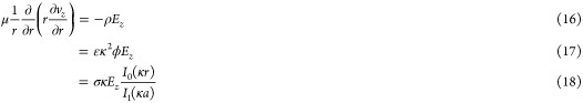where we have used relations from the Poisson and Debye–Hückel equations, and finally our solution for the potential to rewrite the result. Outside the cylinder, the equation is given by

19

We can directly integrate these equations to obtain the final results for the velocity profiles inside and outside the cylinder:

20

and

21

Simulations

Finite-element simulations were carried out using the COMSOL Multiphysics package, version 4.4. The Poisson and Nernst–Planck equations (eqs 1 and 2) are solved in a first step neglecting convection (the c_iu term), which outputs fluxes and concentrations J_i,c, c_i and hence the charge density ρ_e(r) and electric potential ϕ(r). ϕ(r) and ρ_e(r) are the inputs for the body force in the Stokes equation (eq 3), which is solved in a second step to produce the velocity and pressure fields, u(r) and p(r). The ratio of diffusion to convection in the Nernst–Planck equation is approximately D_iz_ieN_Ac_iE_max/(RTu_max) ∼ 10^–6E_max/u_max. In our system E_max ∼ 10⁷ V/m and u_max ∼ 0.1 m/s, giving a diffusive to convective ratio of around 100; thus the neglect of convection in the first step of the simulations is a reasonable approximation. After each run, quantities such as ionic current and flow rate through the pore were calculated. In order to compare with experiments, a quantity P was also extracted by measuring the velocity at a point on the pore axis 1 μm from the pore opening. This simulates placing a bead close to the pore and using it to probe the local velocity (although in reality the measured force is due to an average velocity over the entire bead surface, which is not taken into account here). P is then extracted by applying eq 11 with the appropriate coordinates. Full details are given in Supporting Information S2.

Supporting Information Available

Four figures showing the complete experimental and simulation results, flow profiles for positive and negative voltages, the electric field outside a conical pore, and flow reversal in a finite cylinder; and one description of the COMSOL model. This material is available free of charge via the Internet at http://pubs.acs.org.

The authors declare no competing financial interest.

Funding Statement

National Institutes of Health, United States

References

- Dekker C. Nat. Nanotechnol. 2007, 2, 209–215. [DOI] [PubMed] [Google Scholar]
- Wanunu M. Phys. Life Rev. 2012, 9, 125–158. [DOI] [PMC free article] [PubMed] [Google Scholar]
- Keyser U. F. J. R. Soc. Interface 2011, 8, 1369–1378. [DOI] [PMC free article] [PubMed] [Google Scholar]
- Otto O.; Sturm S.; Laohakunakorn N.; Keyser U. F.; Kroy K. Nat. Commun. 2013, 4, 1780. [DOI] [PMC free article] [PubMed] [Google Scholar]
- Murata K.; Mitsuoka K.; Hirai T.; Walz T.; Agre P.; Heymann J. B.; Engel A.; Fujiyoshi Y. Nature 2000, 407, 599–605. [DOI] [PubMed] [Google Scholar]
- Gravelle S.; Joly L.; Detcheverry F.; Ybert C.; Cottin-Bizonne C.; Bocquet L. Proc. Natl. Acad. Sci. U.S.A. 2013, 110, 16367–16372. [DOI] [PMC free article] [PubMed] [Google Scholar]
- Majumder M.; Chopra N.; Andrews R.; Hinds B. J. Nature 2005, 438, 44. [DOI] [PubMed] [Google Scholar]
- Sparreboom W.; van den Berg A.; Eijkel J. C. T. Nat. Nanotechnol. 2009, 4, 713–720. [DOI] [PubMed] [Google Scholar]
- Johann R.; Renaud P. Electrophoresis 2004, 25, 3720–3729. [DOI] [PubMed] [Google Scholar]
- Glasgow I.; Batton J.; Aubry N. Lab Chip 2004, 4, 558–562. [DOI] [PubMed] [Google Scholar]
- van der Wouden E. J.; Heuser T.; Hermes D. C.; Oosterbroek R. E.; Gardeniers J. G. E.; van den Berg A. Colloids Surf., A 2005, 267, 110–116. [Google Scholar]
- van Dorp S.; Keyser U. F.; Dekker N. H.; Dekker C.; Lemay S. G. Nat. Phys. 2009, 5, 347–351. [Google Scholar]
- Ghosal S. Phys. Rev. Lett. 2007, 98, 238104. [DOI] [PubMed] [Google Scholar]
- Ghosal S. Phys. Rev. E 2007, 76, 061916. [DOI] [PubMed] [Google Scholar]
- Laohakunakorn N.; Ghosal S.; Otto O.; Misiunas K.; Keyser U. F. Nano Lett. 2013, 13, 2798–2802. [DOI] [PubMed] [Google Scholar]
- Wong C. T. A.; Muthukumar M. J. Chem. Phys. 2007, 126, 164903. [DOI] [PubMed] [Google Scholar]
- Laohakunakorn N.; Gollnick B.; Moreno-Herrero F.; Aarts D. G. A. L.; Dullens R. P. A.; Ghosal S.; Keyser U. F. Nano Lett. 2013, 13, 5141–5146. [DOI] [PMC free article] [PubMed] [Google Scholar]
- Squire H. B. Q. J. Mech. Appl. Math. 1951, 4, 321–329. [Google Scholar]
- Otto O.; Steinbock L. J.; Wong D. W.; Gornall J. L.; Keyser U. F. Rev. Sci. Instrum. 2011, 82, 086102. [DOI] [PubMed] [Google Scholar]
- Otto O.; Czerwinski F.; Gornall J. L.; Stober G.; Oddershede L. B.; Seidel R.; Keyser U. F. Opt. Express 2010, 18, 22722–22733. [DOI] [PubMed] [Google Scholar]
- Steinbock L. J.; Otto O.; Chimerel C.; Gornall J.; Keyser U. F. Nano Lett. 2010, 10, 2493–2497. [DOI] [PubMed] [Google Scholar]
- Shevchuk A. I.; Frolenkov G. I.; Sánchez D.; James P. S.; Freedman N.; Lab M. J.; Jones R.; Klenerman D.; Korchev Y. E. Angew. Chem. 2006, 118, 2270–2274. [DOI] [PubMed] [Google Scholar]
- White H. S.; Bund A. Langmuir 2008, 24, 2212–2218. [DOI] [PubMed] [Google Scholar]
- Siwy Z. S. Adv. Funct. Mater. 2006, 16, 735–746. [Google Scholar]
- Schoch R. B.; Han J.; Renaud P. Rev. Mod. Phys. 2008, 80, 839–883. [Google Scholar]
- Kirby B. J.; Hasselbrink E. F. Electrophoresis 2004, 25, 187–202. [DOI] [PubMed] [Google Scholar]
- Behrens S. H.; Grier D. G. J. Chem. Phys. 2001, 115, 6716–6721. [Google Scholar]
- Muthukumar M.Polymer Translocation; CRC Press: Boca Raton, FL, 2011. [Google Scholar]
- Haynes W. M., Bruno T. J., Lide D. R., Eds. CRC Handbook of Chemistry and Physics (Internet Edition), 95th ed.; CRC Press: Boca Raton, FL, 2015. [Google Scholar]
- Smeets R. M. M.; Keyser U. F.; Krapf D.; Wu M.-Y.; Dekker N. H.; Dekker C. Nano Lett. 2006, 6, 89–95. [DOI] [PubMed] [Google Scholar]
- Lee C.; Joly L.; Siria A.; Biance A.-L.; Fulcrand R.; Bocquet L. Nano Lett. 2012, 12, 4037–4044. [DOI] [PubMed] [Google Scholar]
- Stein D.; Kruithof M.; Dekker C. Phys. Rev. Lett. 2004, 93, 035901. [DOI] [PubMed] [Google Scholar]
- Schoch R. B.; Renaud P. Appl. Phys. Lett. 2005, 86, 253111. [Google Scholar]
- Thacker V. V.; Ghosal S.; Hernández-Ainsa S.; Bell N. A. W.; Keyser U. F. Appl. Phys. Lett. 2012, 101, 223704. [DOI] [PMC free article] [PubMed] [Google Scholar]
- Batchelor G. K.An Introduction to Fluid Dynamics; Cambridge University Press: New York, 2000. [Google Scholar]
Associated Data
This section collects any data citations, data availability statements, or supplementary materials included in this article.