Abstract
Although recent guidelines for dealing with missing data emphasize the need for sensitivity analyses, and such analyses have a long history in statistics, universal recommendations for conducting and displaying these analyses are scarce. We propose graphical displays that help formalize and visualize the results of sensitivity analyses, building upon the idea of ‘tipping-point’ analysis for randomized experiments with a binary outcome and a dichotomous treatment. The resulting ‘enhanced tipping-point displays’ are convenient summaries of conclusions obtained from making different modeling assumptions about missingness mechanisms. The primary goal of the displays is to make formal sensitivity analyses more comprehensible to practitioners, thereby helping them assess the robustness of the experiment’s conclusions to plausible missingness mechanisms. We also present a recent example of these enhanced displays in a medical device clinical trial that helped lead to FDA approval.
Keywords: graphical displays, missing data, missing data mechanism, multiple imputation, tipping-point analysis
1. Introduction
Ever since the early work of McKendrick [1], statisticians have been developing methods to account for missing observations in data. Various approaches have been proposed, including weighting observed values by their inverse probability of being observed [2], computing maximum likelihood estimates [3], or imputing each missing value, either once [e.g., 4] or multiple times [5]. Each one of these approaches requires assumptions about the missingness mechanism, implicit or explicit, but, as emphasized by Molenberghs [6], full appreciation was not given to the importance of these assumptions until the mid-70s, when it was proposed in [7] to treat missingness indicators as random variables. It led to the definition of three main missingness mechanisms based on specific assumptions about the distribution of the missingness indicators given data: missing completely at random (MCAR), missing at random (MAR), and missing not at random (MNAR). Detailed definitions of these mechanisms can be found in [8, Section 1.3].
Here, we focus on a special but common case when the univariate binary outcome variable is missing for some units (i.e., partially missing) and a set of predictors that explain the missingness and the outcome is fully observed. Let Y = (y1,…, yN)′, where yi denotes a value of an outcome variable for unit i and let D = (d1,…, dN)′ be the missingness indicator, such that di = 1 for units that are missing yi and di = 0 for units with observed yi. Let X = (xi, j) be the set of predictors, which can be partitioned into three subsets: predictors XY of the response Y only, predictors XD of the missingness indicator D only, and common predictors XYD for Y and D, such that XY, XD, and XYD do not overlap. The triplet (xi, yi, di) is assumed to be independent and exchangeable across units, so we suppress the index i to simplify notation in this section.
Let the conditional probability distribution of the outcome for each unit be
and the conditional probability distribution of the missingness indicator be
where θ and ϕ are vector parameters governing the corresponding distributions. Then, the three missingness mechanisms imply that the following holds for every unit:
MCAR: f(d | xD, xYD, y; ϕ) = f(d | ϕ) for each ϕ and for all x and y. In other words, XD and XYD are empty, and the missingness is independent of the response y itself.
MAR: f(d | xD, xYD, y; ϕ) = f(d | xD, xYD; ϕ) for the observed d, x, and y and for each ϕ.
MNAR: f(d | xD, xYD, y; ϕ) ≠ f(d | xD, xYD ; ϕ). Note that MNAR implies that there are unobserved variables u that are associated with both the response and the missingness indicator, such that f(d | xD, xYD, u, y; ϕ) = f(d | xD, xYD, u ; ϕ), but, because we failed to measure u, the model for the missingness mechanism requires conditioning on the response y itself.
In practice, many studies with missing data either use complete-case analysis (i.e., discard units with partially missing data), which is generally invalid, except in very special cases of MCAR mechanism, or analyze the data under the MAR assumption. The latter is usually regarded as a more sound approach than the former, especially when the MCAR assumption is implausible given observed data. The MAR assumption allows us to avoid specifying a model for missingness mechanism for Bayesian or direct-likelihood inferences, assuming ϕ and θ are distinct [7,8]. However, although the MCAR assumption may be tested empirically [7,9], the MAR assumption is generally unassessable, because it implies comparing f(y | x, d = 0; θ) with f(y | x, d = 1; θ), and the latter can not be estimated from the observed data without making additional assumptions; detailed formalization of this statement is given in [10]. Therefore, a sensitivity analysis is desirable to assess the influence of various assumptions about the missingness mechanism.
Here, focusing on binary outcomes, we describe convenient graphical displays that reveal the effects of all possible combinations of the values of missing data in the first arm (‘treatment’ group) and the second arm (‘control’ group) of a two-arm study on various quantities of interest, typically, on p-values and point estimates. The displays are based on the idea of ‘tipping-point’ (TP) analysis, first introduced in [11], but anticipated in [12–14], as a method of assessing the impact of missing data on study’s conclusions about some quantity of interest. Yan et al. [11] defined tipping points of a study to be particular combinations of missing data values that would change the study’s conclusions, as summarized by its p-value, and presented a simple way to display them. We enhance this idea by formalizing the process of sensitivity analyses using a more detailed display in conjunction with multiple imputation (MI) of missing data. Outputs from multiple formal missingness models, including MNAR ones, are added onto the display along with any historical rates of outcomes, when available. The enhanced displays enable practitioners to identify whether alternative assumptions about the missingness mechanism change the study’s conclusions and thereby allow them to assess the strength of the study’s evidence.
The rest of the manuscript is organized as follows. Section 2 lays out the basics of the sensitivity analysis and the motivation for the proposed technique. Section 3 provides a detailed description of enhanced TP (ETP) displays for a binary outcome. In Section 4, we use a simulated example to demonstrate the display. We then proceed in Section 5 with a real-data example of a recent use of the ETP-displays in a medical device clinical trial and in Section 6 conclude with a discussion.
2. Sensitivity analysis for studies with missing data
A sensitivity analysis consists of several steps:
drawing conclusions under working assumptions about missing data,
identifying a set of plausible alternative assumptions, and
studying the variation in the statistical output and conclusions under these alternative settings.
Because many methods for handling missing data assume a specific MAR mechanism, the last two steps involve using alternative MAR specifications or MNAR mechanisms. However, the majority of empirical studies omit any sensitivity analysis altogether, in part, because of the apparent complexity of such models. Yet, in some cases, omitting it is not an acceptable option, especially when important decisions, such as approving a drug or a medical device or implementing a new public policy are at stake. For example, a recent report on prevention and treatment of missing data, with a focus on clinical trials, produced by the US National Academy of Sciences [15, p. 5], made the following recommendation: ‘Recommendation 15: Sensitivity analyses should be part of the primary reporting of findings from clinical trials. Examining sensitivity to the assumptions about the missing data mechanism should be a mandatory component of reporting.’ Other guidelines issued lately [16–18] also stressed the need to perform sensitivity analyses that assess the impact of missing data on reported inferences and conclusions.
Nevertheless, there is no general agreement as to how one should perform systematic sensitivity analyses and summarize them [15,19]. As pointed out in [15, p. 83], ‘Unlike the well-developed literature on drawing inferences from incomplete data, the literature on the assessment of sensitivity to various assumptions is relatively new. Because it is an active area of research, it is more difficult to identify a clear consensus about how sensitivity analyses should be conducted.’
Recognizing the need for making unassessable assumptions when modeling MNAR missingness, many researchers emphasize the importance of conducting sensitivity analyses and reporting the resulting inferences from different models [e.g., 20–24]. Two general frameworks have been proposed for relaxing the MAR assumption: selection models and pattern-mixture models. With selection models [e.g., 7,25–30], the unassessable assumptions are made about the distribution of outcomes for all units and the distribution of missingness indicators conditional on outcomes, where the parameters for those distributions are distinct. Pattern-mixture models [20,31–34] postulate the distributions of outcomes for respondent and nonrespondents separately, such that the overall outcome distribution is a mixture of the two distributions. Examples of the use of both frameworks can be found in [31,35], in [36–41] for pattern-mixture models, and in [42–47] for selection models. A variant of a pattern-mixture model is used in Section 5 to assess the sensitivity of the estimated treatment effect in a real-data example.
However, few recommendations have been made to help summarize and compare the results of sensitivity analyses across many alternative models of interest, regardless of the framework used. Several authors [12–14] described graphical approaches for summarizing sensitivity analyses, similar to the TP displays proposed in [11] and, also, discussed in [48]. The proposed plots share a common structure, with horizontal and vertical axes defined by some summary of possible values of the outcome for non-respondents in each of two treatment arms, and the plot with shaded areas corresponding to the result of an analysis for each combination of values on the two axes. However, because these previously proposed plots contain no information about the likelihood of each individual combination, we cannot utilize them to their fullest potential. In the following section we introduce ETP-displays, which provide information about the likelihood of each combination and, thereby, of the alternative conclusions.
3. Enhanced tipping-point displays for two-arm randomized studies with binary outcome
Consider a study with N subjects randomly divided into a treatment group of size NT and a control group of size NC, with ti = 1 if subject i is treated and 0 if not treated, T = (t1,…, tN)′. Two vectors of potential outcomes Y(t) = (y1(t),…, yN(t))′, t ∈ {0,1}, indicate whether each subject would be a ‘success’ (yi(t) = 1) or a ‘failure’ (yi(t ) = 0) under treatment assignment t. Under the stable unit treatment values assumption [49, SUTVA,], the observable outcome for subject i can be expressed as
Then, Y = (y1,…, yN)′ is a vector of observable outcomes for the realized treatment assignment vector T.
Let τ be a marginal finite-population average treatment effect
Because the treatment is randomized, an unbiased estimator of τ is
Suppose some subjects are missing the outcome, as indicated by D = (d1,…, dN)′. For a binary outcome Y, a natural marginal summary of missing values is the number of successes among subjects with missing outcomes, considered separately for each arm,
| (1) |
where and . Assuming that the outcome distribution among nonrespondents is binomial, (1) gives the minimum sufficient statistics for the underlying Binomial probabilities of success among nonrespondents.
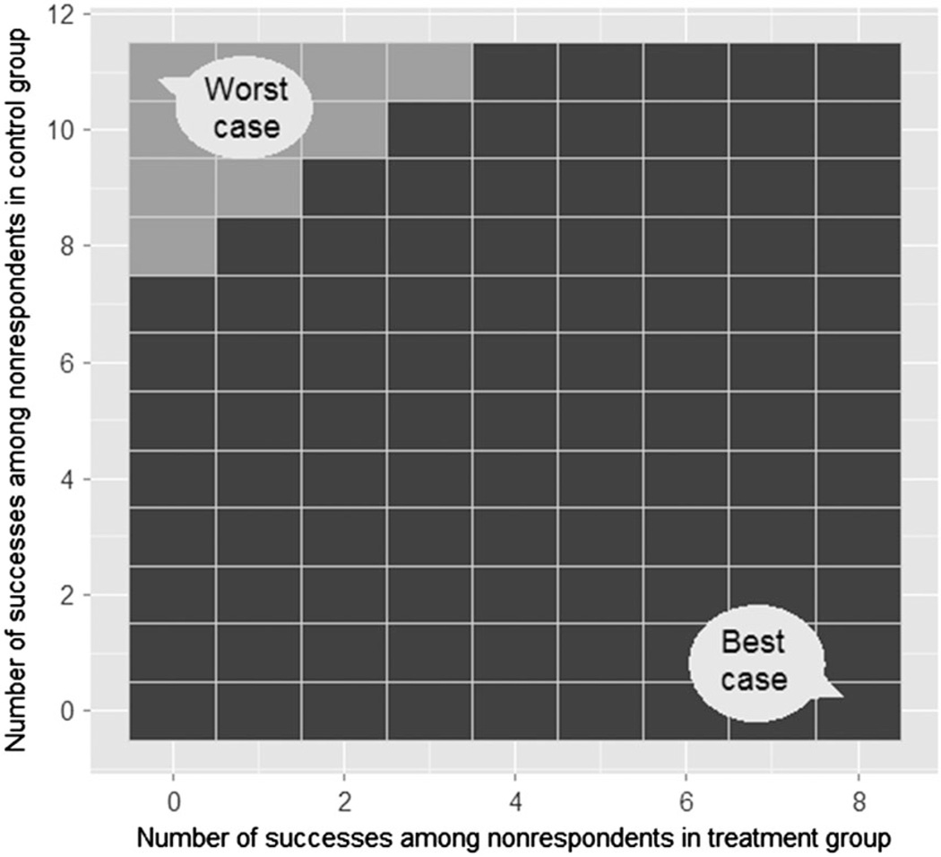
Figure 1 displays a matrix of all possible combinations of the number of successes among nonrespondents in the treatment group, , and in the control group, . Each combination is classified by whether it changes, or ‘tips’, the conclusion about the estimated effect’s statistical significance. The staircase contour partitions the display into two different regions and marks the tipping points of the study, which are the combinations of the number of successes among nonrespondents in the treatment group (horizontal axes) and in the control group (vertical axes) that alter the conclusion about the statistical significance of the estimated treatment effect, based on a chosen hypothesis test and a significance level. A fundamental issue with the basic display is that it has no information about the relative likelihoods of the combinations.
Figure 1.
Basic tipping-point display proposed in [48]. The horizontal and vertical axes indicate the number of successes that can potentially be observed among nonrespondents in the treatment group and the control group. Each combination is marked as either ‘altering the study’s conclusion’ (lighter squares) or ‘keeping the study’s conclusion unchanged’ (darker squares). The staircase region indicates the tipping points of the study.
We extend the idea of such displays by introducing the following enhancements:
- A colored heat map that illustrates the gradual change of a specific quantity of interest, which could be the p-value from a hypothesis test, the estimated treatment effect,
a lower or upper bound of an interval, or any other quantity that depends on the combination of the observed success rates among nonrespondents in the treatment group and in the control group, and .(2) Tick marks on each axis that represent historical estimates of the number of successes in each group, if such are available.
Results from the current modeling procedure, for example, draws of Ymis under the chosen model f(Y, D | T, X; θ, ϕ).
Most important, the draws of Ymis obtained under models with alternative assumptions.
4. Simulated example with a binary outcome
We generated data for N = 100 subjects with two predictors, representing sex, Female = (female1,…, femaleN)′, and age in years, Age = (age1,…, ageN)′, a treatment indicator T = (t1,…, tN)′, and a partially missing binary outcome Y = (y1,…, yN)′ indicating that no adverse events occurred. The predictor Female was simulated from Bern(0.5), and the predictor Age was simulated uniformly between 18 and 55 (rounding to the nearest integer).
The following models were used to generate the outcomes and the missingness:
| (3a) |
| (3b) |
| (3c) |
| (3d) |
where I(·) is an indicator function. According to the notation introduced in Section 1, here XYD = (T, Age, Female), whereas XY and XD are empty. As evident from (3c), the missingness mechanism is MNAR. The model for pi (3a), the probability of success for subject i, indicates that although the treatment effect is positive (i.e., treated subjects had fewer adverse events), the success rates decline steeply for women older than 35 years. The rapid increase in the risk of adverse events after reaching a certain age is not an uncommon phenomenon, for example, the risk of heart disease increases for men after the age of 45 years and for women after the age of 55 years, the risk of having fertility issues (miscarriage, birth defects, etc.) increases for women over the age of 35 years.
In the simulated data, out of the 100 subjects, NT = 40 were randomly assigned to the treatment group and NC = 60 to the control group, with and subjects missing the outcome in each group, respectively. Choosing unequal numbers of treated and control units was intentional to illustrate the generality of the idea. Among the respondents, the success rates were 0.48 (or 12 out of 25) in the treatment group and 0.21 (or 8 out of 39) in the control group.
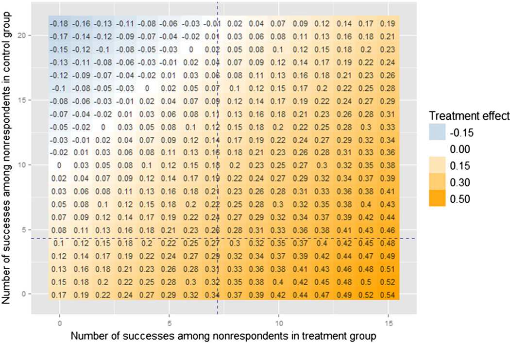
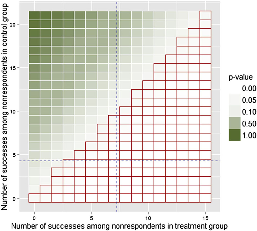
Figure 2 shows the heat map of τ̃ for the generated data set, calculated according to (2). If we perform a one-sided hypothesis test for the difference in proportions of successes between the completed treatment group and the completed control group, the results may also be demonstrated using the ETP-display: Figure 3 shows the heat map of p-values and outlines the region with combinations that resulted in rejecting the null hypothesis that the treatment has a lower rate of success based on the significance level of 0.05. Hence, the outer contour of the region indicates the tipping points of the study, for example, {0,0},{1,1}, or {2,3}. Undoubtedly, the best possible scenario is when the display shows no tipping points, that is, when all combinations of missing outcomes lead to the same conclusion of the study. If this is not the case, as in our simulated example, then performing sensitivity analyses can be critical, and ETP-displays summarize them.
Figure 2.
Enhanced tipping-point display for the simulated binary outcome Y, showing estimated treatment effects using a heat map. Axes represent the number of successes that could be observed among nonrespondents in the treatment group and in the control group. Each combination corresponds to a value of the estimated treatment effect τ̃, according to (2). Its magnitude and sign are represented using a color palette that changes from dark blue (large negative value) to dark orange (large positive values), with white representing zero estimated effect. Note that displaying each individual value is optional (and, in fact, largely redundant), so we omit it in further displays. The axes indicate that there were 15 missing outcomes among treated subjects and 21 among control subjects. Vertical and horizontal dashed lines (in blue) correspond to observed success rates among treated and control subjects, 0.48 and 0.21.
Figure 3.
Enhanced tipping-point display for the simulated binary outcome Y, showing p-values from a chosen hypothesis test (here, a one-sided test of the difference in proportions of successes between treated group and control group). The heat map represents p-values obtained from the test conducted for each combination of the number of successes among treated and among control subjects. The red grid (bottom-right half of the display) highlights combinations that result in rejecting the null hypothesis that the treatment has lower rate of success at the 0.05 significance level, with the staircase region indicating the tipping points of the study.
Next, we illustrate the results of two analyses performed on the simulated data. Both analyses assume a MAR mechanism and multiply impute missing values from their approximate posterior predictive distributions, obtained using multivariate imputation by chained equations (MICE) algorithm [50–52]. The first analysis uses a naïve linear model for the log-odds of success to impute the missing responses, that is, logit(pi) = θ0 + θ1 ti + θ2agei + θ3femalei. The second analysis includes all the relevant interactions, as specified in (3a), and therefore is more complete. Note that the actual details of the imputation procedure are not essential, as long as the procedure is valid and it uses plausible assumptions about the missingness mechanism.
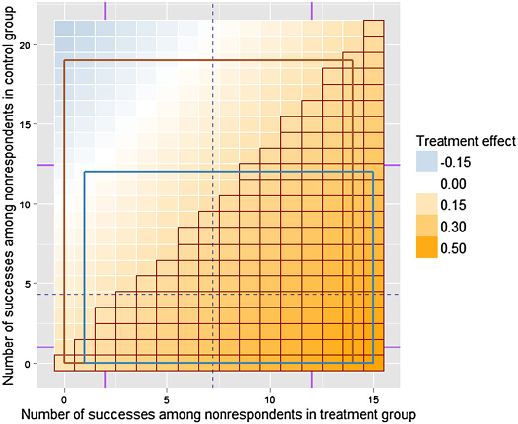
Table I gives the estimates of the treatment effect and its 95% credible intervals (CIs) for each model, combined using Rubin’s rule [5, 53] from 100 generated MIs, as well as the estimate and a 95% CI obtained from the full data. Figure 4 shows the results of the MI procedures from both models‡. Brown and blue rectangles are drawn by connecting minimum and maximum values among 100 imputations in each group under the naïve and the complete models, respectively. The nonparametric intervals formed by minimum and maximum values approximate the 98% CIs for each group, because only 100 simulations were produced (99/101 ≈ 98). Other ways to summarize the joint distribution of successes among non-respondents in treatment group and control group include a 95% credible region based on more simulated values [54] or a kernel density approximation.
Table I.
Treatment effect on the outcome Y, estimated for the full data set and for the observed data set, with missing values multiply imputed using two models: naïve and complete.
| Analysis | Estimated difference | 95% CI |
|---|---|---|
| Full data | 0.27 | (0.09, 0.46) |
| Naïve model | 0.24 | (−0.04, 0.53) |
| Complete model | 0.31 | (0.05, 0.57) |
For both models, we assume MAR missingness and combine results from 100 MIs using Rubin’s rule.
Figure 4.
Enhanced tipping-point display showing the results of two multiple imputation procedures for the simulated binary outcome Y. As before, the red grid highlights combinations that resulted in rejecting the onesided null hypothesis that the treatment has a lower rate of success based on a proportion test, using 0.05 significance level. Rectangles connect minimum and maximum number of successes among 100 imputations for nonrespondents in treatment group and control group under the naïve (brown, taller rectangle) and the complete (blue, shorter rectangle) models, approximating the 98% intervals for each group. Also, the display shows two vertical and two horizontal ticks (in purple), representing counts that correspond to success rates {0.35,0.60} for the treated, and {0.15,0.34} for the controls, the information that might be available from previous studies.
We also added several vertical and horizontal ticks showing counts that correspond to hypothetical historical data. For example, if rates of success for subjects with similar demographics were observed to be 0.35 and 0.60 in previous studies of similar treatments, for our example, they would correspond to having 2 and 12 successes among nonrespondents in the treatment group, respectively.
Figure 4 reveals the differences between counts imputed using the two models. In addition, Table I shows that the two models produce conflicting conclusions regarding the significance of the effect, with the naïve one indicating that there is no significant treatment effect. Note that if additional predictors in the complete model were not associated with both the outcome and the missingness, we would have expected similar results produced under the two models. Next, we describe how a systematic sensitivity analysis was performed on a real data from a medical device clinical trial with multiple binary outcomes and substantial missingness and show how ETP-displays were utilized to summarize the results for a report to FDA.
5. Real-data example with multiple binary outcomes
So far, we focused on the situation with missing values confined to a single binary outcome. However, the example that we now present involves a TP analysis extended to missingness in more than one binary outcome, where some units are missing subsets of outcomes, which may differ across units. This data set is from a clinical trial that studied kyphoplasty, a novel treatment of vertebral compression fractures, which are common complications of osteoporosis, and compared its efficacy and safety to that of vertebroplasty, a current treatment. Both treatments consist of injecting bone cement into fractured vertebrae, with a goal of relieving pain caused by their compression and to prevent further damage.
A randomized prospective open-label study took place in four health centers across Germany. The inclusion criteria for patients required, among other things, to have up to three vertebral compression fractures in a specific region of their spines, to be at least 50 years old, and to have pain levels above a certain threshold. A total of 84 subjects were evaluated, qualified, consented, and randomized to one of the two procedures, yielding 56 subjects assigned to the kyphoplasty (treatment group) and 28 to the vertebroplasty (control group).
The primary endpoint of the study was a number of cement leaks into the spinal canal, a potentially extremely serious complication that can lead to paraplegia. This endpoint, along with pain, was assessed 24 h after the surgery, while patients were still in the hospital. Both variables had no missing data, and we will not focus on them in this section; randomization-based analysis of these endpoints was highly supportive of the superiority of the kyphoplasty procedure performed using the new device.
The study also had several secondary endpoints, including the occurrence of various adverse events within 3 months and between 3 and 12 months after the procedure, which assessed the relative safety of the new device. The following six types of adverse events were recovered:
adjacent level vertebral fracture (symptomatic and asymptomatic),
distant level vertebral fracture (symptomatic and asymptomatic),
retreatment (including re-fracture), and
death.
In addition, subjects’ pain levels (0 through 10) and disability scores (0 through 100, based on a completed questionnaire) were recorded during the 3-month and 12-month follow-up appointments. Table II summarizes all secondary endpoints in the study. In addition, a set of baseline measurements was collected for each patient, including:
the number of vertebral compression fractures that required treatment (1, 2, or 3),
demographic and health data (age, sex, height, weight, BMI, physical activity level, and smoking status), and
baseline pain and disability scores, duration of symptoms, and health center of stay.
Table II.
Secondary endpoints collected in the study, indicated by “+”.
| Time after surgery |
|||
|---|---|---|---|
| Secondary endpoint | At 24 h | 1 day to 3 months | 3 to 12 months |
| Occurrence of each of the six adverse events | + | + | |
| Pain level (0–10) | + | + | + |
| Disability score (0–100) | + | + | |
A considerable fraction of subjects were missing secondary endpoints. Table III reports percents of subjects in each group that had missing outcomes at each time-point. The occurrence of adverse events was rare—the observed rates were between 0% and 2.6%—with the exception of deaths, which were reported at 10.4% rate during the 12 months follow-up; the patients’ age range at baseline was 50–93 years; therefore, such a high death rate was expected. In addition, a few subjects had missingness in one or more of the baseline covariates.
Table III.
Percent of subjects missing all secondary endpoints at each time-point.
| Follow-up time-point |
|||
|---|---|---|---|
| Treatment group | 3 months, % | 12 months, % | 3 & 12 months, % |
| Kyphoplasty (NT = 49)† | 24 | 43 | 18 |
| Vertebroplasty (NC = 28) | 18 | 36 | 11 |
Seven subjects were excluded from the treatment group after randomization because of reasons unrelated to the treatment.
For the purpose of imputation, death is considered to be unrelated to the treatment assigned. Because the death rate was somewhat higher in the control group, by ignoring possible differences between subjects who died and the ones who did not die, the imputation procedure is likely to produce outcomes favorable to the control group, that is, for treated and control subjects with the same covariate values, those who died were more likely to be worse off then those who lived. The procedure is likely to underestimate the rates of adverse events in the control group, making our analysis more ‘conservative’.
Thus, the study had several major missing data issues that complicated the analysis: a considerable fraction of nonmonotone missing data in secondary outcomes that were rare events, some missingness in covariates, and, moreover, small sample sizes. Therefore, regardless of the missingness assumptions that were used for the initial analysis, it was important to perform a thorough sensitivity check.
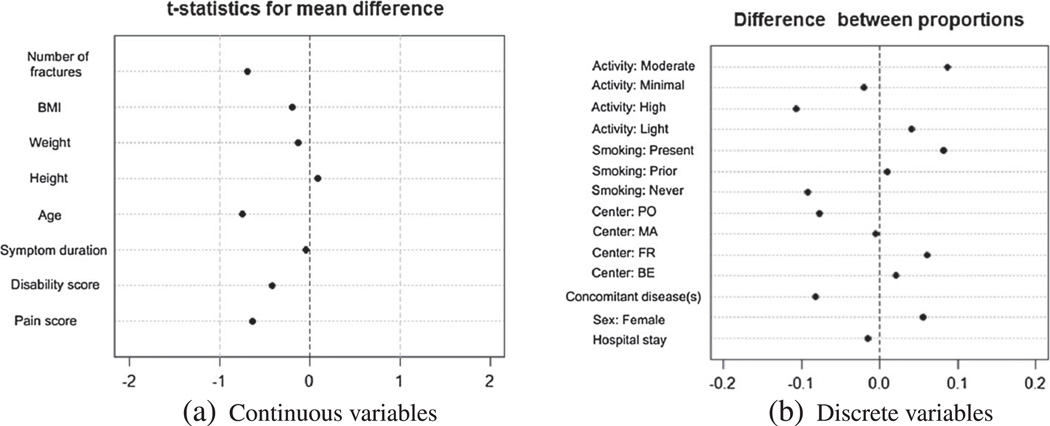
We start with assessing the randomization performance and making sure it produced an acceptable balance between the treatment group and the control group. Figure 5 contains two ‘Love plots’ [55] that show standardized differences between average values of baseline measurements, or between proportions for binary measurements, observed in each group. The two plots indicate excellent balance between the two groups.
Figure 5.
Love plots to check the balance between the treatment group and the control group produced by the randomization. Part (a) shows standardized mean differences for continuous predictors, and part (b) shows differences between raw proportions for categorical predictors.
We proceed with multiply imputing the few missing values in baseline covariates. For that, we combine the two groups, as justified by the randomization, but remove the outcome data. We assume MAR and use the MICE algorithm (based on linear models with main effects only) to produce 100 complete data sets of baseline measurements that will be utilized in subsequent analyses. Next, we describe our assumptions about the missingness mechanism in secondary endpoints, the procedure used for estimating the treatment effect, and the obtained results.
We address the following question regarding secondary endpoints: Do the treatments differ in rates of adverse events or in post-treatment pain levels and disability scores? The approach that we take here is similar to the one used in the Section 3. For the initial analysis, we assume MAR and proceed to multiply impute missing secondary outcomes using MICE, utilizing available baseline covariates. For that, the outcome data collected post-operatively are split into treatment group and control group. Two analysts are assigned to perform MI procedure, one on each group separately; both are blinded to each other’s outcome data. This limits the opportunity to bias the results, for example, by systematically imputing better values for subjects in the treatment group, as well as to allow different response functions for outcomes in each group.
The sparsity of adverse events requires a special method of conditional imputation because it is not feasible to model the occurrence of each of twelve adverse events (six types of events at two time-points) individually. Instead, we use a hot-deck approach by adopting a file-concatenation matching method introduced in [56], where each subject with missing secondary outcomes (i.e., a nonrespondent) is matched based on available characteristics to a donor from a pool of respondents, and the entire set of outcomes from the chosen donor is used to impute missing outcomes for that nonrespondent. In addition, post-treatment pain scores and disability indexes, collected during the 3-month and 12-month follow-up appointments cannot be modeled as continuous variables because of small sample size and irregular distributions of the observed values. Therefore, for the purpose of MI, we employ predictive mean matching [56, PMM,; 57], another hot-deck-type method that fits a linear model to observed responses and uses it to match each nonrespondent with a set of respondents.
To test whether or not the treatment group and control group showed similar results in secondary outcomes, we employ a one-sided Fisher randomization test. Table IV reports results obtained from 100 completed data sets, combined using Rubin’s rule as described in [58]. These results support the conclusion that there is essentially no evidence that kyphoplasty, performed using the new device, is worse than vertebroplasty in the rate of any adverse event, as well as in average post-treatment pain scores or disability indexes. Next, we subject these conclusions to a thorough sensitivity assessment.
Table IV.
One-sided p-values from a Fisher randomization test for null hypotheses of no difference between the treatment group and the control group in the rate of each of the adverse events.
| Alternative hypothesis | Treated subjects have fewer adverse events | |
|---|---|---|
| Adverse events | With 3 months | Between 3 and 12 months |
| Retreatment | 1.00 | 1.00 |
| Symptomatic adjacent fracture | 0.30 | 1.00 |
| Symptomatic distant fracture | 0.99 | 0.27 |
| Asymptomatic adjacent fracture | 1.00 | 0.99 |
| Asymptomatic distant fracture | 1.00 | 0.48 |
| Death | 0.13 | 0.59 |
| Any event before 3 months | 0.29 | 0.32 |
| Pain score | 0.66 | 0.29 |
| Disability index | 0.26 | 0.19 |
| Alternative hypothesis | Treated subjects have more adverse events | |
| Adverse events | With 3 months | Between 3 and 12 months |
| Retreatment | 0.39 | 0.99 |
| Symptomatic adjacent fracture | 0.89 | 0.46 |
| Symptomatic distant fracture | 0.38 | 0.99 |
| Asymptomatic adjacent fracture | 1.00 | 1.00 |
| Asymptomatic distant fracture | 1.00 | 0.90 |
| Death | 0.99 | 0.68 |
| Any event before 3 months | 0.83 | 0.80 |
| Pain score | 0.34 | 0.71 |
| Disability index | 0.75 | 0.82 |
A one-sided alternative hypothesis was used to make it possible to combine the p-values from 100 complete data sets [58]. Note that none of the p-values provide any evidence against the corresponding null hypotheses.
The generally unassessable MAR assumption that underlies the imputations of missing secondary endpoints raises concerns because of the large fraction of missing values. Also, the hot-deck imputation methods used for secondary endpoints were drawing outcomes that were actually observed, and an implicit assumption of such methods is that each nonrespondent resembles one or more of the respondents. However, further analysis revealed that there was some nonoverlap in the values of baseline measurements between respondents and nonrespondents in the control group. Specifically,
- At the 3-month follow-up:
-
–all three male nonrespondents were older than the oldest male respondent (76, 77, 83 vs. 69 years old at the beginning of the study);
-
–two out of three male nonrespondents had lower BMI than the lowest observed BMI among respondents (21.5, 20 vs. 23.5 kg/m2);
-
–one out of two female nonrespondents had prior smoking experience, and no female respondent had any; and
-
–one male nonrespondent had a longer hospital stay duration than all male respondents.
-
–
- At the 12-month follow-up:
-
–two female nonrespondents were older than the oldest female respondent (88, 89 vs. 85 years old); and
-
–one male nonrespondent was older than the oldest male respondent (83 vs. 77 years).
-
–
Note that the nonrespondents who did not resemble any respondents in the control group appeared to be in poorer health than the respondents, for example, older and with low BMI. Consequently, by using responses from healthier subjects in the control group to impute missing outcomes for nonrespondents, the hot-deck imputation procedure produces results favoring the control group. Nevertheless, the detection of nonoverlap provided us with a direction for constructing MNAR models: identify specific characteristic of nonrespondents that are outside of the range observed among respondents and modify the odds of adverse events for subjects with these characteristics, taking the odds estimated under the MAR model as a baseline
where δ(ti, xi) is an introduced shift that may depend on subject’s i treatment assignment, ti, and baseline values, xi. The following eight characteristics were selected for the purpose of this sensitivity analysis: men older than 69 years, men with BMI lower than 23.5, women with prior smoking experience, men with duration of hospital stay longer than 2 days, women older than 85 years, men older than 77 years, patients dead at 3 months, and patients dead at 12 months. The odds of not having adverse events were imputed to be 50% higher (δ = ln (1.5)) or 50% lower (δ = ln (0.5)) than implied by the MAR model for the treatment group or the control group separately.
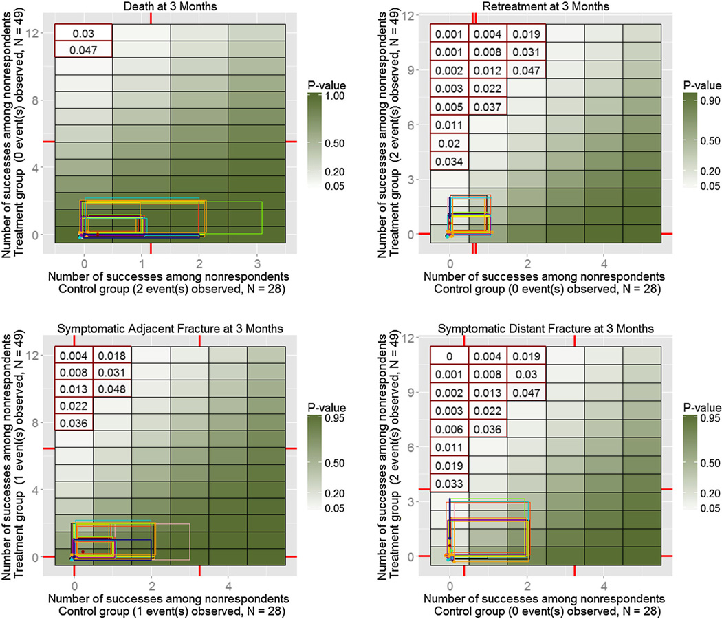
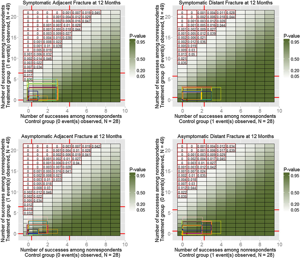
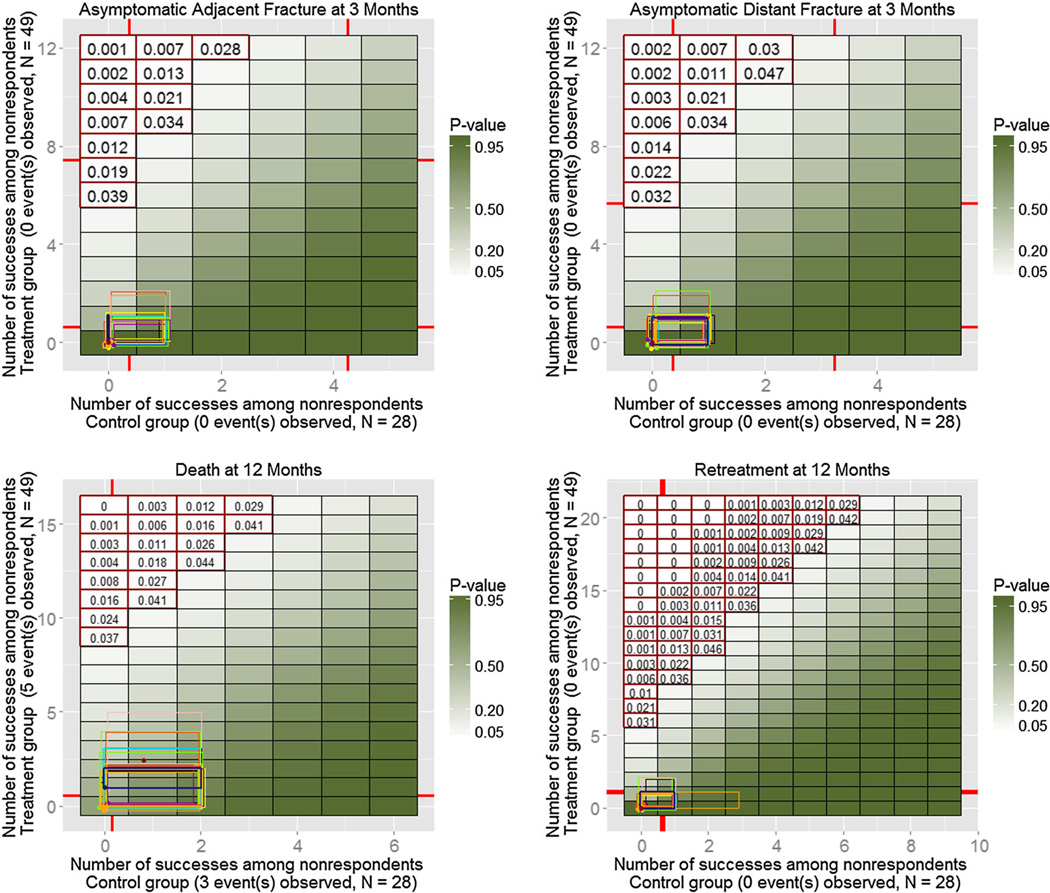
A total of 32 alternative models were fitted (eight characteristics for two groups and two odds adjustments), and 100 MIs were produced for each of them. Similarly to the simulated example on Figure 4, Figures 6–8 show resulting ETP-displays with rectangles indicating ranges of the number of adverse events imputed under the initial model with the MAR assumption (dark blue), as well as under each of the 32 alternative models. The heat map represents p-values for one-sided Fisher randomization tests with alternative hypothesis that treated subjects have higher rates of adverse events than control subjects. Historical values obtained from experts are marked on each axis, and tipping points of the study, based on a 0.05 significance level, are highlighted using red contour.
Figure 6.
Enhanced tipping-point displays for the first four adverse events from the clinical trial described in Section 5, with (jittered) rectangles showing ranges of the number of adverse events for nonrespondents in treatment group and control group, imputed under the MAR assumption (thick blue rectangle), as well as under each of the 32 alternative models chosen for the sensitivity analysis. None of the models resulted in changes in the study’s conclusions.
Figure 8.
Enhanced tipping-point displays for the last four adverse events from the clinical trial described in Section 5. Only a couple of models for the adjacent symptomatic fractures (top left) produced borderline results.
It is evident from displays that the study conclusion is robust to all alternative models explored here; none of the rectangular areas cover the TP contour on any of the 12 displays. These ETP-displays reassure us that there is no evidence for differences in safety between the new kyphoplasty device and the traditional vertebroplasty procedure. Considering that the analysis of primary endpoints indicated a considerable advantage of the new device over the current procedure, our TP analysis and displays helped to advance the approval of the device by the FDA.
6. Discussion
We proposed a systematic way to summarize sensitivity analyses in a randomized two-arm study with one or more binary outcomes that are partially missing using ETP graphical displays. The displays facilitate the assessment of the strength of study’s conclusions under adopted assumptions and inform us about the effect of alternative models on the initial conclusions. They systematize sensitivity analyses by taking advantage of fast computing to create MIs under the current and alternative models and to display results using modern computational graphics.
Sometimes, when assessing the impact of missing data on a study’s conclusion, researches focus on the worst-case scenario, that is, treated subjects with missing outcomes are assumed to have zero favorable outcomes and, at the same time, missing outcomes for controls are set to be all favorable. In fact, in the simulated example shown in Section 4, this scenario would reverse the sign of the treatment effect, as it is evident from Figure 4. Among the advantages of the ETP-displays is that they allow the assessment of other intermediate combinations, which usually are more realistic than the worst-case scenario. Moreover, the displays can help to convey the fact that the worst-case scenario may likely be unachievable, even if alternative assumptions, including MNAR, about missing data mechanism are employed. Finally, ETP-displays show the posterior probability of each combination, thereby helping to assess the influence of alternative assumptions on the study’s conclusions. An R-procedure for ETP-displays is available at sites. google.com/site/vliublinska/research.
In the real-data example in Section 5, we tackled several issues at once, including substantial missingness in the outcomes with small sample sizes in treatment and control groups. A thorough sensitivity check is a key step in this situation, exploring plausible models with alternative assumptions about the nature of missingness mechanism, including MNAR ones. An intuitive way to explore MNAR models is to use the fitted outcome model under the MAR assumption as a baseline and introduce various modifications for the nonrespondents’ model, informed by experts in the field. In addition, by summarizing imputation results on ETP-displays, investigators can identify alternative models that are most likely to tip the study’s conclusions. This idea can be generalized to studies with other types of outcomes. It provides a new collection of useful tools for the analysis of data sets plagued with missing values.
Figure 7.
Enhanced tipping-point displays for the next four adverse events from the clinical trial described in Section 5. Again, all models lead to the same conclusion of no difference in rates of adverse events between the treatment group and the control group.
Acknowledgements
We thank Professor Roee Gutman for the helpful discussions and for assisting in the implementation of the imputation procedure; Soteira, Inc. for permission to use their data, and Dr. Gregory Campbell for pointing us to the original publication on related TP analysis.
Footnotes
The R-procedure that draws ETP-displays for generated MIs can be downloaded from sites.google.com/site/vliublinska/research.
References
- 1.M’Kendrick AG. Applications of mathematics to medical problems. Proceedings of the Edinburgh Mathematical Society. 1925;44:98–130. [Google Scholar]
- 2.Horvitz DG, Thompson DJ. A generalization of sampling without replacement from a finite universe. Journal of the American Statistical Association. 1952;47(260):663–685. [Google Scholar]
- 3.Dempster AP, Laird NM, Rubin DB. Maximum likelihood from incomplete data via the EM algorithm Journal of the Royal Statistical Society. Series B (Methodological) 1977;39(1):1–38. [Google Scholar]
- 4.Healy M, Westmacott M. Missing values in experiments analysed on automatic computers Journal of the Royal Statistical Society. Series C (Applied Statistics) 1956;5(3):203–206. [Google Scholar]
- 5.Rubin DB. Multiple Imputation for Nonresponse in Surveys. 1st ed. New York: Wiley; 1987. [Google Scholar]
- 6.Molenberghs G. Editorial: what to do with missing data? Journal of the Royal Statistical Society. Series A (Statistics in Society) 2007;170(4):861–863. [Google Scholar]
- 7.Rubin DB. Inference and missing data. Biometrika. 1976;63(3):581–592. [Google Scholar]
- 8.Little RJA, Rubin DB. Statistical Analysis with Missing Data. 2nd ed. New York: Wiley; 2002. [Google Scholar]
- 9.Little RJA. A test of missing completely at random for multivariate data with missing values. Journal of the American Statistical Association. 1988;83(404):1198–1202. [Google Scholar]
- 10.Mealli F, Rubin DB. Missing at random for independent and identically distributed variables. Biometrika. 2014 [Google Scholar]
- 11.Yan X, Lee S, Li N. Missing data handling methods in medical device clinical trials. Journal of Biopharmaceutical Statistics. 2009;19(6):1085–1098. doi: 10.1080/10543400903243009. [DOI] [PubMed] [Google Scholar]
- 12.Matts JP, Launer CA, Nelson ET, Miller C, Dain B. A graphical assessment of the potential impact of losses to follow-up on the validity of study results. Statistics in Medicine. 1997;16(17):1943–1954. doi: 10.1002/(sici)1097-0258(19970915)16:17<1943::aid-sim631>3.0.co;2-r. [DOI] [PubMed] [Google Scholar]
- 13.Hollis S. A graphical sensitivity analysis for clinical trials with non-ignorable missing binary outcome. Statistics in Medicine. 2002;21(24):3823–3834. doi: 10.1002/sim.1276. [DOI] [PubMed] [Google Scholar]
- 14.Weatherall M, Pickering Rm, Harris S. Graphical sensitivity analysis with different methods of imputation for a trial with probable non-ignorable missing data. Australian & New Zealand Journal of Statistics. 2009;51(4):397–413. [Google Scholar]
- 15.NRC-Panel. The Prevention and Treatment of Missing Data in Clinical Trials. Washington, DC: National Academies Press; 2010. [PubMed] [Google Scholar]
- 16.Burzykowski T, Carpenter J, Coens C, Evans D, France L, Kenward M, Lane P, Matcham J, Morgan D, Phillips A, Roger J, Sullivan B, White I, Yu LyM. Missing data: discussion points from the PSI missing data expert group. Pharmaceutical Statistics. 2010;9(4):288–297. doi: 10.1002/pst.391. [DOI] [PubMed] [Google Scholar]
- 17.CHMP. Guideline on missing data in confirmatory clinical trials, Technical Report. European Medical Agency; 2010. [Google Scholar]
- 18.Methodology committee of the patient-centered outcomes research institute. PCORI methodology standards. 2012. [Google Scholar]
- 19.Lee SY. Handbook of Latent Variable and Related Models. Amsterdam: Elsevier; 2007. [Google Scholar]
- 20.Rubin DB. Formalizing subjective notions about the effect of nonrespondents in sample surveys. Journal of the American Statistical Association. 1977;72(359):538–543. [Google Scholar]
- 21.Rosenbaum PR, Rubin DB. Assessing sensitivity to an unobserved binary covariate in an observational study with binary outcome Journal of the Royal Statistical Society. Series B (Methodological) 1983;45(2):212–218. [Google Scholar]
- 22.Scharfstein DO, Rotnitzky A, Robins JM. Adjusting for nonignorable drop-out using semiparametric nonresponse models. Journal of the American Statistical Association. 1999;94(448):1096–1120. [Google Scholar]
- 23.Verbeke G, Molenberghs G. Linear Mixed Models for Longitudinal Data. 1st ed. New York: Springer; 2000. [Google Scholar]
- 24.Rotnitzky A, Scharfstein D, Su TL, Robins J. Methods for conducting sensitivity analysis of trials with potentially nonignorable competing causes of censoring. Biometrics. 2001;57(1):103–113. doi: 10.1111/j.0006-341x.2001.00103.x. [DOI] [PubMed] [Google Scholar]
- 25.Heckman JJ. The common structure of statistical models of truncation, sample selection and limited dependent variables and a simple estimator for such models, Technical Report NBER Chapters. National Bureau of Economic Research, Inc; 1976. [Google Scholar]
- 26.Rubin DB. Multiple imputations in sample surveys-a phenomenological bayesian approach to nonresponse; Proceedings of the Section on Survey Research Methods of the American Statistical Association; 1978. pp. 20–34. [Google Scholar]
- 27.Rubin DB. Imputation and editing of faulty or missing survey data. Washington, DC: U.S. Department of Commerce; 1978. The phenomenological bayesian perspective in sample surveys from finite populations: Foundations; pp. 10–18. [Google Scholar]
- 28.Little RJA, Rubin DB. Statistical Analysis with Missing Data. 1st ed. New York: Wiley; 1987. [Google Scholar]
- 29.Diggle P, Kenward MG. Informative drop-out in longitudinal data analysis Journal of the Royal Statistical Society. Series C (Applied Statistics) 1994;43(1):49–93. [Google Scholar]
- 30.Robins JM, Rotnitzky A, Scharfstein DO. Sensitivity analysis for selection bias and unmeasured confounding in missing data and causal inference models. In: Halloran ME, Berry DA, editors. Statistical models in epidemiology, the environment and clinical trials. New York: Springer; 2000. p. 192. [Google Scholar]
- 31.Glynn RJ, Laird NM, Rubin DB. Drawing inferences from self-selected samples. Mahwah, NJ, US: Lawrence Erlbaum Associates Publishers; 1986. Selection modeling versus mixture modeling with nonignorable nonresponse; pp. 115–142. [Google Scholar]
- 32.Little RJA. Pattern-mixture models for multivariate incomplete data. Journal of the American Statistical Association. 1993;88(421):125–134. [Google Scholar]
- 33.Little RJA, Wang Y. Pattern-mixture models for multivariate incomplete data with covariates. Biometrics. 1996;52(1):98–111. [PubMed] [Google Scholar]
- 34.Daniels MJ, Hogan JW. Reparameterizing the pattern mixture model for sensitivity analyses under informative dropout. Biometrics. 2000;56(4):1241–1248. doi: 10.1111/j.0006-341x.2000.01241.x. [DOI] [PubMed] [Google Scholar]
- 35.Wu MC, Bailey K. Analysing changes in the presence of informative right censoring caused by death and withdrawal. Statistics in Medicine. 1988;7(1–2):337–346. doi: 10.1002/sim.4780070134. [DOI] [PubMed] [Google Scholar]
- 36.Wu MC, Bailey KR. Estimation and comparison of changes in the presence of informative right censoring: conditional linear model. Biometrics. 1989;45(3):939–955. [PubMed] [Google Scholar]
- 37.Hogan JW, Laird NM. Mixture models for the joint distribution of repeated measures and event times. Statistics in Medicine. 1997;16(3):239–257. doi: 10.1002/(sici)1097-0258(19970215)16:3<239::aid-sim483>3.0.co;2-x. [DOI] [PubMed] [Google Scholar]
- 38.Hedeker D, Gibbons RD. Application of random-effects pattern-mixture models for missing data in longitudinal studies. Psychological Methods. 1997;2(1):64–78. [Google Scholar]
- 39.Hogan JW, Laird NM. Increasing efficiency from censored survival data by using random effects to model longitudinal covariates. Statistical Methods in Medical Research. 1998;7(1):28–48. doi: 10.1177/096228029800700104. [DOI] [PubMed] [Google Scholar]
- 40.Ekholm A, Skinner C. The muscatine children’s obesity data reanalysed using pattern mixture models. Journal of the Royal Statistical Society: Series C (Applied Statistics) 1998;47(2):251–263. [Google Scholar]
- 41.Thijs H, Molenberghs G, Michiels B, Verbeke G, Curran D. Strategies to fit pattern mixture models. Biostatistics. 2002;3(2):245–265. doi: 10.1093/biostatistics/3.2.245. [DOI] [PubMed] [Google Scholar]
- 42.Wu MC, Carroll RJ. Estimation and comparison of changes in the presence of informative right censoring by modeling the censoring process. Biometrics. 1988;44(1):175–188. [Google Scholar]
- 43.Glynn RJ, Laird NM, Rubin DB. Multiple imputation in mixture models for nonignorable nonresponse with follow-ups. Journal of the American Statistical Association. 1993;88(423):984–993. [Google Scholar]
- 44.Molenberghs G, Kenward MG, Lesaffre E. The analysis of longitudinal ordinal data with nonrandom drop-out. Biometrika. 1997;84(1):33–44. [Google Scholar]
- 45.Rotnitzky A, Robins JM, Scharfstein DO. Semiparametric regression for repeated outcomes with nonignorable nonre-sponse. Journal of the American Statistical Association. 1998;93(444):1321–1339. [Google Scholar]
- 46.Scharfstein DO, Daniels MJ, Robins JM. Incorporating prior beliefs about selection bias into the analysis of randomized trials with missing outcomes. Biostatistics. 2003;4(4):495–512. doi: 10.1093/biostatistics/4.4.495. [DOI] [PMC free article] [PubMed] [Google Scholar]
- 47.Minini P, Chavance M. Sensitivity analysis of longitudinal normal data with drop-outs. Statistics in Medicine. 2004;23(7):1039–1054. doi: 10.1002/sim.1702. [DOI] [PubMed] [Google Scholar]
- 48.Campbell G, Pennello G, Yue L. Missing data in the regulation of medical devices. Journal of Biopharmaceutical Statistics. 2011–02;21(2):180–195. doi: 10.1080/10543406.2011.550094. [DOI] [PubMed] [Google Scholar]
- 49.Rubin DB. Randomization analysis of experimental data: the fisher randomization test comment. Journal of the American Statistical Association. 1980;75(371):591–593. [Google Scholar]
- 50.Rubin DB. Nested multiple imputation of NMES via partially incompatible MCMC. Statistica Neerlandica. 2003;57(1):3–18. [Google Scholar]
- 51.Buuren van S, Groothuis-Oudshoorn K. MICE: multivariate imputation by chained equations in R. Journal of Statistical Software. 2011;45(3):1–67. [Google Scholar]
- 52.Buuren Sv. Flexible Imputation of Missing Data. 1st ed. Hoboken: Chapman and Hall/CRC; 2012. [Google Scholar]
- 53.Barnard J, Rubin DB. Small-sample degrees of freedom with multiple imputation. Biometrika. 1999;86(4):948–955. [Google Scholar]
- 54.Held L. Simultaneous posterior probability statements from Monte Carlo output. Journal of Computational and Graphical Statistics. 2004;13(1):20–35. [Google Scholar]
- 55.Ahmed A, Husain A, Love TE, Gambassi G, Dell’Italia LJ, Francis GS, Gheorghiade M, Allman RM, Meleth S, Bourge RC. Heart failure, chronic diuretic use, and increase in mortality and hospitalization: an observational study using propensity score methods. European Heart Journal. 2006;27(12):1431–1439. doi: 10.1093/eurheartj/ehi890. [DOI] [PMC free article] [PubMed] [Google Scholar]
- 56.Rubin DB. Statistical matching using file concatenation with adjusted weights and multiple imputations. Journal of Business & Economic Statistics. 1986;4(1):87–94. [Google Scholar]
- 57.Little RJA. Missing-data adjustments in large surveys. Journal of Business & Economic Statistics. 1988;6(3):287–296. [Google Scholar]
- 58.Licht C. Ph.D. Thesis. Otto-Friedrich-Universitat; 2010. New methods for generating significance levels from multiply-imputed data. [Google Scholar]


