

Abstract
Purpose:
In magnetic resonance-guided focused ultrasound (MRgFUS) therapies, the in situ characterization of the focal spot location and quality is critical. MR acoustic radiation force imaging (MR-ARFI) is a technique that measures the tissue displacement caused by the radiation force exerted by the ultrasound beam. This work presents a new technique to model the displacements caused by the radiation force of an ultrasound beam in a homogeneous tissue model.
Methods:
When a steady-state point-source force acts internally in an infinite homogeneous medium, the displacement of the material in all directions is given by the Somigliana elastostatic tensor. The radiation force field, which is caused by absorption and reflection of the incident ultrasound intensity pattern, will be spatially distributed, and the tensor formulation takes the form of a convolution of a 3D Green’s function with the force field. The dynamic accumulation of MR phase during the ultrasound pulse can be theoretically accounted for through a time-of-arrival weighting of the Green’s function. This theoretical model was evaluated experimentally in gelatin phantoms of varied stiffness (125-, 175-, and 250-bloom). The acoustic and mechanical properties of the phantoms used as parameters of the model were measured using independent techniques. Displacements at focal depths of 30- and 45-mm in the phantoms were measured by a 3D spin echo MR-ARFI segmented-EPI sequence.
Results:
The simulated displacements agreed with the MR-ARFI measured displacements for all bloom values and focal depths with a normalized RMS difference of 0.055 (range 0.028–0.12). The displacement magnitude decreased and the displacement pattern broadened with increased bloom value for both focal depths, as predicted by the theory.
Conclusions:
A new technique that models the displacements caused by the radiation force of an ultrasound beam in a homogeneous tissue model theory has been rigorously validated through comparison with experimentally obtained 3D displacement data in homogeneous gelatin phantoms using a 3D MR-ARFI sequence. The agreement of the experimentally measured and simulated results demonstrates the potential to use MR-ARFI displacement data in MRgFUS therapies.
Keywords: MRgFUS, MR-ARFI, radiation force modeling
1. INTRODUCTION
Magnetic resonance-guided focused ultrasound (MRgFUS) is a noninvasive technology that is able to treat a range of pathologies. Applications include the treatment of solid tumors1–3 and neurological disorders,4,5 localized drug delivery,6,7 opening the blood brain barrier,8,9 sonoporation,10,11 and thrombolysis.12,13 Because this technology is noninvasive, the in situ characterization of the focal spot location and its quality is critical. It has been shown that ultrasound beam aberrations, which can affect both the accurate placement and quality of the focal spot, are particularly pronounced after transmission through strongly aberrating structures such as the ribs or skull.14 It has also been reported that beam aberrations can be significant in other tissues such as the breast.15,16
In MRgFUS therapy, the focal spot can be assessed by visualizing the temperature rise produced by an interrogative heating pulse using MR thermometry. While this has been used successfully clinically,17,18 there are disadvantages. It may be necessary to repeat this localization technique several times during a treatment, potentially depositing unwanted energy in the surrounding healthy tissues. In addition, obtaining significant temperature increases may be difficult in highly perfused regions, and the proton resonance frequency shift technique, a common method for MR temperature imaging, is not temperature sensitive in fat.19
Magnetic resonance acoustic radiation force imaging (MR-ARFI) is a technique that measures the tissue displacement caused by the force exerted by the focused ultrasound beam. This displacement map, generally acquired with MR signals in a 2D plane perpendicular to the ultrasound beam, provides information about the position and quality of the focal spot that is complementary to MR thermometry information and can therefore be useful during all aspects of MRgFUS therapy.20
During the pretreatment phase, MR-ARFI can assess the focus and targeting quality of the ultrasound beam. Several developed MR-ARFI sequences have demonstrated the ability for both beam localization and adaptive focusing.20–23 These techniques have been expanded to applications that include motion. For example, Holbrook et al.24 used a gated spin echo flyback EPI sequence with repeated bipolar motion-encoding gradients (MEG) to demonstrate that MR-ARFI can be used for beam localization in a free-breathing in vivo porcine model, while Auboiroux et al.25 demonstrated a gradient echo-EPI sequence with alternating bipolar MEGs that simultaneously measures both displacement and temperature in a mechanically ventilated in vivo sheep model.
In addition to beam characterization, MR-ARFI has also been used for the correction of phase aberration. It has been found that the phase aberration correction obtained from using empirical MR-ARFI measurements results in a more intense and sharpened focal spot when compared with the correction computed using a segmented skull model obtained from computed tomography (CT) images.21,26–29
Finally, MR-ARFI can be used in the post-treatment phase to assess the change of mechanical properties of the treated tissue. Bitton et al.30 found that the MR-ARFI-measured peak displacement in previously ablated regions in human cadaver breasts decreased by approximately 55%. While this result opposes the increase of displacement measured after ablation of ex vivo bovine kidney reported in Ref. 20 both papers found that a change was detectable after tissue ablation.
Various investigators have simulated the displacement field due to an acoustic radiation force. Walker31 used a Green’s function analysis to compute the displacements along the axis of the beam in several homogeneous tissue types by assuming an infinite isotropic medium with the force field modeled as a series of closely spaced disks of varying radii. Bercoff et al.32 developed a model that accounts for compressional, shear, and coupling waves in viscoelastic media and found that the theory fit the experimental data well with ultrasound pulses on the order of microseconds. This model was applied by other investigators in a rat brain.33 Sarvazyan et al.34 presented a theory to model shear wave elasticity imaging derived from the KZK equation and was the first to demonstrate the experimental MRI encoding of ARFI. Others have solved the weak form of the 3D elastodynamic equations using a finite-element modeling analysis35 or have applied a broadening filter to the simulated ultrasound intensity pattern.29 An overdamped response model to relate the tissue motion due to the acoustic radiation force to the duration of the ultrasound pulse has also been presented.28,36
This paper presents a new technique to model the displacements caused by the radiation force of an ultrasound beam in a homogeneous tissue model mapped to a full 3D Cartesian grid. While several other theories have been presented, the model used in this work was developed specifically for use for MR-ARFI applications where the ultrasound pulse duration is typically on the order of several milliseconds. The presented model only incorporates physical tissue parameters and therefore does not require identification of tissue response estimations. The theory behind the technique and experimental validation in several homogeneous phantom models with independently measured acoustic and mechanical properties are presented.
2. MODELING ARFI DISPLACEMENTS
2.A. Acoustic beam and force modeling
The radiation force acting on a medium through which an acoustic beam propagates is due to medium-induced changes in the momentum carried by the beam. This momentum alteration can be caused by partial absorption of the beam’s energy, partial reflection of the ultrasound beam at a tissue interface, or both.37 Since this work deals with homogeneous models, only the absorptive portion of the beam’s energy will be addressed. If the time-average intensity of the beam is I (W/m2) and the pressure absorption coefficient of the medium is α (Np/m), the radiation force volume density due to absorption Γa (N/m3) is given by35
| (1) |
where c (m/s) is the speed of sound in the medium.
In order to calculate the radiation force pattern in an irradiated medium using Eq. (1) the pattern of the beam’s intensity I must first be found. The beam propagation simulations in this study use a rapid computational method called the hybrid angular spectrum (HAS) technique.38 This approach defines the acoustic properties of the propagation medium on a regularly spaced 3D Cartesian grid with grid spacing Δx, Δy, and Δz (m) along each coordinate axis; z is the direction of beam propagation. Each voxel in the model contains unique values for speed of sound c, absorp tion α, and density ρ. After finding the pressure from the transducer through water to the front face of the model using the traditional Rayleigh–Sommerfeld integral,39 the pressure pattern is then progressively calculated in the z-direction through sequential x-y layers of the model, first in the space domain, then in the spatial-frequency domain for each layer. First-order pressure reflections are also calculated at each layer interface. In this way, the entire steady-state 3D pattern for pressure p (N/m2) is derived and the time-average intensity pattern is found as40
| (2) |
where Z is the acoustic impedance (kg/m2 s). Once the intensity pattern is known, the force F (N) in each voxel can be calculated. The force due to absorption within voxel i is
| (3) |
Considering the spatial resolution of the model, this force is ascribed to a point at the center of voxel i. The 3D force pattern is thus obtained for the entire model.
2.B. Displacement modeling
The MR-ARFI displacement modeling technique developed in this paper assumes that the medium in which the force is generated is homogeneous and infinite in extent. Linear isotropic elastic properties of the medium and steady-state, or elastostatic, conditions on the displacement are also assumed—with one accommodation for the dynamic behavior of the displacement, as explained in Sec. 2.C.
When a steady-state-force point source acts internally in an infinite homogeneous medium, the displacement of the material in the neighborhood of the point source is given by the Somigliana elastostatic tensor31,41,42 for an arbitrary force magnitude and direction and considering displacements along all three axes. However, in ARFI the force is predominantly in the direction of the beam propagation and the displacement of interest is in this same direction. Considering only displacements in the beam propagation direction, the Somigliana tensor reduces to a form that gives displacement w (mm) in the z-direction in terms of the force magnitude F and the two Lamé constants λ and μ (N/mm2),
| (4) |
where
| (5) |
r (mm) is the length of vector from the point source to the location of w, and z (mm) is the projection of this vector onto the z-axis.
Almost all tissues can be considered to be nearly incompressible with a Poisson’s ratio σ very close to 0.5.43 Since the Lamé constants λ (first constant) and μ (shear constant) are related by
| (6) |
in most tissues, λ > > μ,44 and Eqs. (4) and (5) reduce to
| (7) |
where
| (8) |
and
| (9) |
Equation (7) describes the z-displacement for a single point source of force. To obtain the accumulated displacements for a distribution of forces throughout the medium, Eq. (7) can be extended to be the convolution of a 3D Green’s function with the 3D force field pattern F obtained from Eq. (3) as discussed in Sec. 2.C. A plot of the spatial extent of , the term in the Green’s function that describes its spatial variation, is shown in Fig. 1(a) for an x-z plane centered on the point force.
FIG. 1.

(a) Plot of the central portion of [Eq. (9)], showing the value of the Green’s function describing its spatial variation on the model’s Cartesian grid. Shown is an x − z plane view where z is the ultrasound propagation direction. Isotropic grid spacing is assumed throughout this paper, so Δx = Δy = Δz = b. (b) To find a working value for the Green’s function in its central voxel, the force F is assumed uniformly distributed throughout the voxel cross-sectional area ΔxΔy = b2 perpendicular to the force direction, and is convolved with the resulting force density F/b2 over this area. The result is g(0) = 3.52/b.
2.C. Computational implementation
Convolution is most efficiently carried out computationally in the spatial-frequency domain by multiplying the spectra of the two components.45 We do this in matlab by first finding the 3D fast Fourier transform (fftn, matlab function) of both the force pattern and the Green’s function to obtain their respective spectra, multiplying these complex spectra element-by-element, then performing an inverse Fourier transform (ifftn, matlab function) on the result to find the displacement w.
Two practical considerations must be addressed: (1) The vector extends from the center of the voxel where the particular point force component is located to the center of each neighboring voxel, as shown in Fig. 1(a). The length r of this center-to-center vector and the corresponding value of z are used to evaluate the Green’s function [Eq. (9)] for all voxels outside the central voxel where the point force is located. However, in the central voxel, the Green’s function has an infinite singularity, since r = 0 at that point. To find a finite value for the displacement to attribute to this source voxel, we let the force be uniformly distributed over the ΔxΔy = b2 cross-sectional area of the voxel perpendicular to the force direction, yielding a force density of F/b2, where b = 0.5 mm for all simulations. We then integrate this force density with the Green’s function (with z = 0) to compute the convolution over the cross-sectional area to find w(0). As shown in Fig. 1(b), the integration is given by multiplying the result for the shaded triangular segment by a factor of 8,
| (10) |
where Eq. (259) in Ref. 46 was used to find the value for the definite integral. Therefore, the term of the Green’s function that describes its spatial variation, , is given a value of 3.52/b in the central voxel, as shown in Fig. 1(a).
(2) While the theory used in this study assumes that elastostatic conditions exist, it is known that the radiofrequency phase change resulting from the displacement accumulates dynamically during the encoding duration of the MR-ARFI sequence [φ(t) in Eq. (11)], which is the same as the duration of the ultrasound radiation force (10 ms) for our simulations and experiments. To account for this dynamic accumulation of phase during the MR encoding duration, our numerical implementation assumes that this displacement at a given point does not occur until the shear wavefront—which propagates spherically with speed β = √(μ/ρ) away from each source point42—reaches that location after initiation of the ultrasound pulse. We implemented this effect by multiplying the Green’s function with a weighting function that decreases linearly from one at r = 0 to zero at a radius that is the product of the ultrasound exposure time and the shear wave speed (radii = 23, 53, and 86 mm for the 125-, 175-, and 250-bloom phantoms, respectively). This consequently reduces the width and height of the resulting displacement pattern. This time-of-arrival weighting is applied to in the space domain before transformation and convolution in the frequency domain. This assumption and its implications are addressed further in Sec. 5.
3. EXPERIMENTAL METHODS
3.A. Tissue-mimicking phantoms
Experimental validation of the displacement calculations provided by the HAS-ARFI simulations was done using gelatin-based phantoms (Vyse Gelatin Co. and Sigma-Aldrich Corp.) of various bloom numbers. The bloom number corresponds to the stiffness of the phantom material; higher bloom values equate to a more stiff material.35 Three bloom values (125-, 175-, and 250-bloom) were used for validation in this study. All phantoms were fabricated between 3 and 18 h prior to the MR-ARFI experimental measurements, acoustic measurements, and Young’s modulus testing; all testing was done at nominal room temperature.
The speed of sound and attenuation coefficient for each phantom was determined using a through transmission technique.47,48 The density for all phantom samples was found to be 1060 ± 36 kg/m3. The Young’s modulus of each of the three bloom-valued materials was measured in unconfined compression using an Instron 5944 single column testing system. The mean and standard deviation of 12 measurements for each bloom is reported in Table I. The Lamé shear constant μ is related to Young’s modulus E by the equation when Poisson’s ratio σ is nearly 0.5; this allows calculation of the shear wave speed from β = √(μ/ρ).
TABLE I.
Relevant parameters for the gelatin phantoms. The mean and standard deviation are shown for all measured values.
| Phantom bloom value | Attenuation (dB/cm MHz) N = 3 | Speed of sound (m/s) N = 3 | Young’s modulus (kPa) N = 12 | Calculated shear wave speed (m/s) |
|---|---|---|---|---|
| 125 | 0.52 ± 0.05 | 1553 ± 26 | 8.2 ± 0.1 | 2.6 |
| 175 | 0.55 ± 0.08 | 1549 ± 18 | 17.0 ± 0.8 | 5.3 |
| 250 | 0.57 ± 0.05 | 1553 ± 12 | 26.3 ± 2.0 | 8.3 |
3.B. MRgFUS procedures
All experiments were performed with a magnetic resonance-guided focused ultrasound system (Image Guided Therapy, Inc.) in a Siemens Trio 3 Tesla MRI scanner. The 256-element phased-array ultrasound transducer was operated at 1 MHz. A schematic of the experimental setup is shown in Fig. 2. Displacements in the phantom were measured using a 3D spin echo segmented-EPI sequence with unbalanced bipolar motion-encoding gradients and flyback readout as shown in Fig. 3 [repetition time = 250 ms, echo time = 60 ms, flip angle = 90°, echo train length = 7, 256 × 128 × 36-mm field of view, 2 × 2 × 3-mm acquired voxel resolution zero-filled interpolated to 0.5 × 0.5 × 0.5-mm voxel spacing, motion-encoding gradient amplitude = 30 mT/m, motion-encoding gradient duration = 10 ms, ultrasound pulse duration (USdur) = 10 ms, ultrasound acoustic power = 66 W, and acquisition time = 32 s]. The sequence was repeated with ultrasound off and on, giving a phase difference only proportional to ultrasound induced displacement.49
FIG. 2.

Schematic of the gelatin phantom in the MRgFUS system. The placement of the slice group is within the dashed rectangle and the direction of the motion-encoding gradient (MEG) is shown. The coordinate system origin is placed centrally in the phantom at its bottom face.
FIG. 3.

Schematic of the 3D segmented-EPI spin echo sequence with unbalanced bipolar motion-encoding gradients.
The displacement is proportional to the accumulated radiofrequency phase change and can be determined from the following relationship:
| (11) |
where w(t′) (μm) is the displacement, φ is the phase change (rad), γ is the gyromagnetic ratio (MHz/T), and MEG (T/m) is the applied motion-encoding gradient as a function of the ultrasound duration time (USdur). Equation (11) can be simplified by assuming that the displacement time course, given by ς(t) for unit displacement, is independent of peak displacement amplitude (wpeak)
| (12) |
For the phantoms in this work, the high shear wave velocities calculated for these phantoms (2.6–8.3 m/s) indicate that the tissue response time is much shorter than 10 ms, and the temporal function, ς(t), is very close to unity during the MEG gradient and is set to unity in this work.
For each displacement measurement, a total of nine measurements (total acquisition time = 288 s) were acquired interleaving ultrasound OFF- and ON-images, beginning and ending the acquisition series with OFF-images. The two OFF-images before and after each ON-image were averaged to account for any potential field drift that may have occurred during the ON-image acquisition. The four resulting displacement images were averaged to generate a final displace ment map for each ultrasound sonication.
Experiments were performed in nine phantoms (three at each bloom value). Since the applied force field is a function of absorption [Eq. (1)], experiments were performed at two depths, 30 or 45 mm from the phantom’s bottom face. In total, 11 sonications were applied at the 30-mm depth and six sonications were applied at the 45-mm depth for each bloom value. In phantoms 1, 4, and 7, these sonications were applied at different locations in a single plane in the phantom, approximately 2.5-cm apart in a cross pattern. This was done to evaluate any boundary condition effects. Sonications were all applied at the same location for all other cases. These sonications were divided among the three phantoms of each given bloom value, as indicated in Table III.
TABLE III.
MR-ARFI displacement results for all phantoms. The mean and standard deviation of the measured peak displacement are shown.
| Phantom bloom value | Depth into phantom (mm) | Phantom number | Number of sonications | Mean of peak displacement (μm) | Standard deviation of peak displacement (μm) |
|---|---|---|---|---|---|
| 125 | 30 | 1 | 5 | 17.43 | 2.24 (12.9%) |
| 2 | 3 | 35.36 | 3.24 (9.2%) | ||
| 3 | 3 | 24.89 | 1.79 (7.2%) | ||
| 45 | 2 | 3 | 25.06 | 1.02 (4.1%) | |
| 3 | 3 | 15.31 | 1.77 (11.6%) | ||
| 175 | 30 | 4 | 5 | 14.10 | 1.08 (7.7%) |
| 5 | 3 | 12.05 | 1.01 (8.4%) | ||
| 6 | 3 | 10.63 | 1.51 (14.2%) | ||
| 45 | 5 | 3 | 11.29 | 0.87 (7.7%) | |
| 6 | 3 | 6.47 | 1.49 (23.0%) | ||
| 250 | 30 | 7 | 5 | 8.55 | 1.14 (13.3%) |
| 8 | 3 | 14.65 | 1.42 (9.7%) | ||
| 9 | 3 | 7.26 | 0.91 (12.5%) | ||
| 45 | 8 | 3 | 14.19 | 1.33 (9.4%) | |
| 9 | 3 | 6.46 | 1.55 (24.0%) |
The measured experimental and simulated displacement values were compared using a normalized root mean squared difference (diffRMS)
| (13) |
where wex and wsim are the experimentally measured and simulated displacements, respectively, summed over the N voxels in a 35 × 35 × 35-mm cube centered on the peak displacement point. The variable wsim,peak is the peak displacement found throughout the simulated volume.
4. RESULTS
The mean of the maximum displacement profiles measured in all phantoms fabricated with a specific bloom value is shown in Fig. 4. The displacement profiles at both the 30- and 45-mm penetration depths are plotted along the x-axis (see Fig. 2 for orientation) at the z-axis value of maximum displacement. The error bars represent one standard deviation. Figure 5 displays the same measurements plotted along the z-axis in the direction of ultrasound propagation passing through the location of peak displacement. When comparing the data across all phantoms, one standard deviation ranges from 12% to 38% of the peak displacement mean.
FIG. 4.
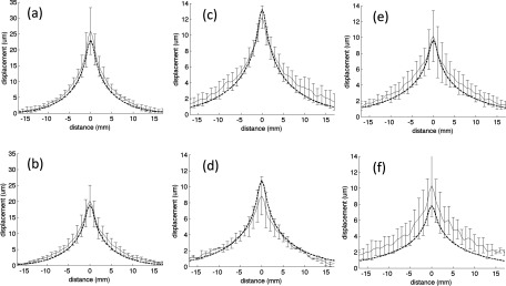
Mean of all peak experimental displacement profiles along the x-direction at 30- (a), (c), and (e) and 45-mm (b), (d), and (f) focal depths into the (a) and (b) 125-, (c) and (d) 175-, and (e) and (f) 250-bloom phantoms. The error bars (shown every-other measurement point) represent one standard deviation. The overlaid dashed lines show the simulated displacements.
FIG. 5.

Mean of all peak experimental displacement profiles along the z-direction at 30- (a), (c), and (e) and 45-mm (b), (d), and (f) focal depths into the (a) and (b) 125-, (c) and (d) 175-, and (e) and (f) 250-bloom phantoms. The error bars (shown every-other measurement point) represent one standard deviation. The overlaid dashed lines show the simulated displacements.
Simulation results for all phantom bloom values at both penetration depths are also shown in Figs. 4 and 5 as dashed lines overlaid on the experimental data. The simulations were generated following the procedure outlined in Sec. 2 using the mean Young’s modulus and acoustic properties listed in Table I. Each simulation to calculate the intensity pattern took approximately 20 s on a 2.0-GHz dual-core Windows XP laptop with 4 GB of RAM, plus 12 s to calculate the resulting displacement pattern. The normalized root-mean-squared difference between the simulated and experimentally measured displacement values is shown in Table II for the various experimental cases. The distance between the position of the peak displacement in the experimental and simulated results (Δwsim,exp) is also shown.
TABLE II.
RMS difference between the MR-ARFI experimental displacements and the simulated displacements.
| Phantom bloom value | 125 | 175 | 250 | |||
|---|---|---|---|---|---|---|
| Depth into phantom (mm) | 30 | 45 | 30 | 45 | 30 | 45 |
| diffRMS | 0.028 | 0.052 | 0.052 | 0.041 | 0.036 | 0.12 |
| Δwsim,exp (mm) | 0.20 | 0.17 | 0.82 | 0.64 | 0.70 | 1.15 |
Figure 6 illustrates slice views through the center of the focal zone of the 125-bloom phantom at 30-mm focal depth for both the experimentally derived displacement pattern and the simulated pattern, providing a 2D comparison between the two results for this typical case. The difference maps between the experimentally measured and simulated displacement patterns are also shown. The displayed region corresponds to the same volume over which the diffRMS value was calculated (35 × 35 × 35 mm).
FIG. 6.
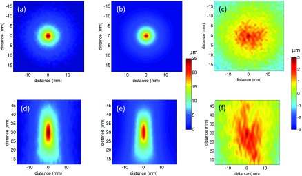
Displacement maps from the 125-bloom phantom at a 30-mm penetration depth both perpendicular (a) and (b) and parallel (d) and (e) to the axis of ultrasound beam propagation for the experimental (a) and (d) and simulated (b) and (e) data. The difference between the experimental and simulated data is shown for both orientations (c) and (f). Note the different scales for (a), (b), (d), and (e), and for (c) and (f).
An overall comparison of the mean maximum displacement profiles of all blooms is shown in Fig. 7. As expected, as the bloom value increases, the peak displacement decreases in both the experimental and simulated data. In addition, an increase of bloom value, representing an increase in the Young’s modulus and thus the Lamé shear coefficient, causes the shape of the displacement pattern to broaden in both the experimental and simulated data since the shear wave speed increases, as discussed in Sec. 5.
FIG. 7.

Mean of all peak experimental displacements (solid lines) along the x-direction at a 30-mm penetration depth for the 125- (black), 175- (red), and 250-bloom (blue) phantoms. The overlaid dashed lines of the same color are the simulated displacements.
The mean and standard deviation of the peak displacement measured in each of the nine total phantoms are shown in Table III. Evaluation of the intravariability in a single phantom shows that one standard deviation ranges from about 4%–24% of the mean peak displacement, giving an indication of the repeatability of the measurement data. The peak displacement measurements between different phantoms of the same bloom at the same penetration depth show that the intervariability of the displacement was much higher in different phantoms of the same bloom value.
5. DISCUSSION
The results presented in this study demonstrate that the displacement resulting from the acoustic radiation force of a focused ultrasound beam can be accurately modeled in homogeneous gelatin phantoms with independently measured acoustic and varying stiffness values. While in vivo values strongly depend on frequency, the values used in this work are comparable to those found in in vivo tissues.50–53 The results shown in Figs. 4, 5, and 7 and Table II demonstrate the ability of the technique to predict the magnitude of the displacement as well as the overall shape. The 3D MR-ARFI sequence implemented allows rigorous comparison of the simulated results to experimentally obtained data.
The assumptions of linear, isotropic material properties and of a nearly incompressible material (thus λ > > μ) have greatly simplified the expressions describing the displacements and appear to be reasonable for the cases studied. However, the assumption of elastostatic conditions requires further discussion. When a point force is imposed in an elastic medium, both longitudinal and shear wavefronts radiate spherically from that point.42 When λ > > μ, as in the media here, the speed of the longitudinal wavefront is much faster than the shear wave, but its displacement amplitude is very much smaller; the major displacement is associated with the arrival of the shear wave component. Thus, the MRI phase changes related to displacement do not start to appreciably accumulate at any location until the shear wave component, moving at the shear wave speed β, reaches that location from the point force.
The model presented in this work differs from models presented by other investigators as we have not directly addressed the effect of the media’s viscous properties on the shear wave propagation. Some investigators have directly included viscous effects32,33 while others have used a more simplified model to account for the noninstantaneous tissue response.28,36 In order to account for the noninstantaneous tissue response, we assumed that displacement due to the shear wave component did not occur until the shear wave reached that point. This was implemented by applying a weighting factor to the Green’s function whose extent was a function of the shear wave speed. The validity of this technique is apparent in Fig. 7 where the stiffer phantoms with a higher shear wave speed have wider displacement profiles. While this technique would not be effective in applications where the ultrasound pulse duration is short32,33 (0.2–3 ms), it is a reasonable assumption in this application since the ultrasound beam’s intensity is constant for a reasonably long time (10 ms). This assumption simplifies the model allowing for easier implementation while still resulting in accurate modeling of ARFI displacement patterns in homogeneous phantoms.
The accuracy of the model was tested by comparing simulated and measured data over a range of phantoms of varied stiffness. The experimental data showed that interphantom variability was significantly larger than the intraphantom variability for all phantom bloom values despite the fact that all phantoms of the same bloom number were fabricated from the same lot of gelatin using the same protocol. While we attempted to minimize the variability of the timing between phantom fabrication and testing as well as the temperature of the phantom at the time of testing, both of these variables most likely contributed to the higher interphantom variability in the measured displacement.54 While all phantoms in this study were approximately at room temperature at the beginning of the MR-ARFI experiment, there was likely some variability (although the absolute temperature of the phantom was not measured during the experimental protocol). In addition, variations in temperature can occur not only due to variations in initial temperature but also from heating due to radiofrequency energy from the MRI coil and oscillating gradients. It is also possible that the phantom could have increased in temperature during each MR-ARFI sonication. In prior studies by our group, magnetic resonance temperature imaging determined that the 3D ARFI sequence parameters used in this study would result in a 3 °C–6 °C peak temperature rise in the gelatin phantoms.
The trends present in both the experimental and simulated displacement results correspond with the theoretical predictions. For example, an increased bloom number corresponds to a stiffer material with a larger Young’s modulus (and therefore a larger Lamé shear coefficient). Since the amplitude of the 3D force field for a given focal depth is relatively insensitive to the bloom number (all bloom values had similar acoustic properties), Eq. (7) predicts an inverse relationship between bloom number and the extent of the displacements. A comparison of both the measured and simulated displacements at 30-mm penetration depth at the three bloom values in Fig. 7 shows that the displacement does decrease with increasing phantom bloom value, as predicted. In addition, as the phantom bloom value increases, the shear wave speed in the phantom also increases, causing a broadening of the overall displacement pattern. The displacement pattern of the 250-bloom phantom is significantly broader than the 125-bloom phantom in both the measured and predicted data. Also, increasing the penetration depth from 30- to 45-mm decreases the magnitude of the force pattern generated by the ultrasound beam due to increased beam attenuation, resulting in a decreased displacement. This can be seen in both Figs. 4 and 5 for both the simulated and experimental data.
Although the theory presented in this work assumes a homogeneous infinite medium, the hybrid angular spectrum algorithm that is used to calculate the ultrasound intensity pattern is designed to predict intensity patterns for heterogeneous models. The calculation of heterogeneous ARFI displacement patterns will require special treatment at all boundaries of differing Lamé constants and is beyond the scope of this work. However, since the ultrasound intensity pattern can be computed throughout models with heterogeneity, the displacements in larger regions of interests of relative homogeneity could be potentially predicted using this technique.
6. CONCLUSIONS
A new technique that models the displacements caused by the radiation force of an ultrasound beam in a homogeneous tissue model has been presented. The theory has been rigorously validated through comparison with experimentally obtained 3D displacement data using a 3D MR-ARFI sequence in homogeneous gelatin phantoms. These promising results demonstrate the potential to use MR-ARFI displacement data in MRgFUS therapies. Possible applications include using this technique to optimize MR-ARFI sequences for clinical use, assessing the pathological state of tissues after ablation treatments, and localizing and assessing the focal spot during focused ultrasound therapies and phase aberration correction methods.
ACKNOWLEDGMENTS
This work was supported by NIH Grant Nos. R01 EB013433 and R01 HL172787.
REFERENCES
- 1.McDannold N., Tempany C. M., Fennessy F. M., So M. J., Rybicki F. J., Stewart E. A., Jolesz F. A., and Hynynen K., “Uterine leiomyomas: MR imaging-based thermometry and thermal dosimetry during focused ultrasound thermal ablation,” Radiology 240(1), 263–272 (2006). 10.1148/radiol.2401050717 [DOI] [PMC free article] [PubMed] [Google Scholar]
- 2.Furusawa H., Namba K., Thomsen S., Akiyama F., Bendet A., Tanaka C., Yasuda Y., and Nakahara H., “Magnetic resonance-guided focused ultrasound surgery of breast cancer: Reliability and effectiveness,” J. Am. Coll. Surg. 203(1), 54–63 (2006). 10.1016/j.jamcollsurg.2006.04.002 [DOI] [PubMed] [Google Scholar]
- 3.Wu F., “Extracorporeal high intensity focused ultrasound in the treatment of patients with solid malignancy,” Minim. Invasive Ther. Allied Technol. 15(1), 26–35 (2006). 10.1080/13645700500470124 [DOI] [PubMed] [Google Scholar]
- 4.Lipsman N., Schwartz M. L., Huang Y., Lee L., Sankar T., Chapman M., Hynynen K., and Lozano A. M., “MR-guided focused ultrasound thalamotomy for essential tremor: A proof-of-concept study,” Lancet Neurol. 12(5), 462–468 (2013). 10.1016/S1474-4422(13)70048-6 [DOI] [PubMed] [Google Scholar]
- 5.Elias J. W., Huss D., Khaled M. A., Monteith S. J., Frysinger R., and Loomba J., “MR-guided focused ultrasound lesioning for the treatment of essential tremor–A new paradigm for noninvasive lesioning and neuromodulation,” Congress of Neurological Surgeons, Washington, DC, October 1–6, 2011. [Google Scholar]
- 6.Rapoport N., Nam K. H., Gupta R., Gao Z., Mohan P., Payne A., Todd N., Liu X., Kim T., Shea J., Scaife C., Parker D. L., Jeong E. K., and Kennedy A. M., “Ultrasound-mediated tumor imaging and nanotherapy using drug loaded, block copolymer stabilized perfluorocarbon nanoemulsions,” J. Controlled Release 153(1), 4–15 (2011). 10.1016/j.jconrel.2011.01.022 [DOI] [PMC free article] [PubMed] [Google Scholar]
- 7.Frenkel V., Etherington A., Greene M., Quijano J., Xie J., Hunter F., Dromi S., and Li K. C., “Delivery of liposomal doxorubicin (Doxil) in a breast cancer tumor model: Investigation of potential enhancement by pulsed-high intensity focused ultrasound exposure,” Acad. Radiol. 13(4), 469–479 (2006). 10.1016/j.acra.2005.08.024 [DOI] [PubMed] [Google Scholar]
- 8.McDannold N., Arvanitis C. D., Vykhodtseva N., and Livingstone M. S., “Temporary disruption of the blood–brain barrier by use of ultrasound and microbubbles: Safety and efficacy evaluation in rhesus macaques,” Cancer Res. 72(14), 3652–3663 (2012). 10.1158/0008-5472.CAN-12-0128 [DOI] [PMC free article] [PubMed] [Google Scholar]
- 9.Hynynen K., McDannold N., Vykhodtseva N., Raymond S., Weissleder R., Jolesz F. A., and Sheikov N., “Focal disruption of the blood–brain barrier due to 260-kHz ultrasound bursts: A method for molecular imaging and targeted drug delivery,” J Neurosurg. 105(3), 445–454 (2006). 10.3171/jns.2006.105.3.445 [DOI] [PubMed] [Google Scholar]
- 10.Qiu Y., Zhang C., Tu J., and Zhang D., “Microbubble-induced sonoporation involved in ultrasound-mediated DNA transfection in vitro at low acoustic pressures,” J. Biomech. 45(8), 1339–1345 (2012). 10.1016/j.jbiomech.2012.03.011 [DOI] [PubMed] [Google Scholar]
- 11.Van Ruijssevelt L., Smirnov P., Yudina A., Bouchaud V., Voisin P., and Moonen C., “Observations on the viability of C6-glioma cells after sonoporation with low-intensity ultrasound and microbubbles,” IEEE Trans. Ultrason. Ferroelectr. Freq. Control. 60(1), 34–45 (2013). 10.1109/TUFFC.2013.2535 [DOI] [PubMed] [Google Scholar]
- 12.Shaw G. J., Meunier J. M., Huang S. L., Lindsell C. J., McPherson D. D., and Holland C. K., “Ultrasound-enhanced thrombolysis with tPA-loaded echogenic liposomes,” Thromb. Res. 124(3), 306–310 (2009). 10.1016/j.thromres.2009.01.008 [DOI] [PMC free article] [PubMed] [Google Scholar]
- 13.Jones G., Hunter F., Hancock H. A., Kapoor A., Stone M. J., Wood B. J., Xie J., Dreher M. R., and Frenkel V., “In vitro investigations into enhancement of tPA bioavailability in whole blood clots using pulsed-high intensity focused ultrasound exposures,” IEEE Trans. Biomed. Eng. 57(1), 33–36 (2010). 10.1109/TBME.2009.2028316 [DOI] [PMC free article] [PubMed] [Google Scholar]
- 14.Hynynen K. and Sun J., “Trans-skull ultrasound therapy: The feasibility of using image-derived skull thickness information to correct the phase distortion,” IEEE Trans. Ultrason. Ferroelectr. Freq. Control. 46(3), 752–755 (1999). 10.1109/58.764862 [DOI] [PubMed] [Google Scholar]
- 15.Mougenot C., Tillander M., Koskela J., Kohler M. O., Moonen C., and Ries M., “High intensity focused ultrasound with large aperture transducers: A MRI based focal point correction for tissue heterogeneity,” Med. Phys. 39(4), 1936–1945 (2012). 10.1118/1.3693051 [DOI] [PubMed] [Google Scholar]
- 16.Farrer A., Almquist S., Parker D., Christensen D., and Payne A., “Assess ment and correction of phase aberrations in the breast for MRgFUS,” 13th International Symposium for Therapeutic Ultrasound, Shanghai, China, May 12–16, 2013. [Google Scholar]
- 17.McDannold N., Clement G. T., Black P., Jolesz F., and Hynynen K., “Transcranial magnetic resonance imaging- guided focused ultrasound surgery of brain tumors: Initial findings in 3 patients,” Neurosurgery 66(2), 323–332 (2010). 10.1227/01.NEU.0000360379.95800.2F [DOI] [PMC free article] [PubMed] [Google Scholar]
- 18.Fennessy F. M., Tempany C. M., McDannold N. J., So M. J., Hesley G., Gostout B., Kim H. S., Holland G. A., Sarti D. A., Hynynen K., Jolesz F. A., and Stewart E. A., “Uterine leiomyomas: MR imaging-guided focused ultrasound surgery–results of different treatment protocols,” Radiology 243(3), 885–893 (2007). 10.1148/radiol.2433060267 [DOI] [PubMed] [Google Scholar]
- 19.Hynynen K., Pomeroy O., Smith D. N., Huber P. E., McDannold N. J., Kettenbach J., Baum J., Singer S., and Jolesz F. A., “MR imaging-guided focused ultrasound surgery of fibroadenomas in the breast: A feasibility study,” Radiology 219(1), 176–185 (2001). 10.1148/radiology.219.1.r01ap02176 [DOI] [PubMed] [Google Scholar]
- 20.McDannold N. and Maier S. E., “Magnetic resonance acoustic radiation force imaging,” Med. Phys. 35(8), 3748–3758 (2008). 10.1118/1.2956712 [DOI] [PMC free article] [PubMed] [Google Scholar]
- 21.Larrat B., Pernot M., Montaldo G., Fink M., and Tanter M., “MR-guided adaptive focusing of ultrasound,” IEEE Trans. Ultrason. Ferroelectr. Freq. Control. 57(8), 1734–1737 (2010). 10.1109/TUFFC.2010.1612 [DOI] [PMC free article] [PubMed] [Google Scholar]
- 22.Chen J., Watkins R., and Pauly K. B., “Optimization of encoding gradients for MR-ARFI,” Magn. Reson. Med. 63(4), 1050–1058 (2010). 10.1002/mrm.22299 [DOI] [PMC free article] [PubMed] [Google Scholar]
- 23.Kaye E. A., Chen J., and Pauly K. B., “Rapid MR-ARFI method for focal spot localization during focused ultrasound therapy,” Magn. Reson. Med. 65(3), 738–743 (2011). 10.1002/mrm.22662 [DOI] [PMC free article] [PubMed] [Google Scholar]
- 24.Holbrook A. B., Ghanouni P., Santos J. M., Medan Y., and Paulye K. B., “In vivo MR acoustic radiation force imaging in the porcine liver,” Med. Phys. 38(9), 5081–5089 (2011). 10.1118/1.3622610 [DOI] [PMC free article] [PubMed] [Google Scholar]
- 25.Auboiroux V., Viallon M., Roland J., Hyacinthe J. N., Petrusca L., Morel D. R., Goget T., Terraz S., Gross P., Becker C. D., and Salomir R., “ARFI-prepared MRgHIFU in liver: Simultaneous mapping of ARFI-displacement and temperature elevation, using a fast GRE-EPI sequence,” Magn. Reson. Med. 68(3), 932–946 (2012). 10.1002/mrm.23309 [DOI] [PubMed] [Google Scholar]
- 26.Hertzberg Y., Volovick A., Zur Y., Medan Y., Vitek S., and Navon G., “Ultrasound focusing using magnetic resonance acoustic radiation force imaging: Application to ultrasound transcranial therapy,” Med. Phys. 37(6), 2934–2942 (2010). 10.1118/1.3395553 [DOI] [PubMed] [Google Scholar]
- 27.Marsac L., Chauvet D., Larrat B., Pernot M., Robert B., Fink M., Boch A. L., Aubry J. F., and Tanter M., “MR-guided adaptive focusing of therapeutic ultrasound beams in the human head,” Med. Phys. 39(2), 1141–1149 (2012). 10.1118/1.3678988 [DOI] [PMC free article] [PubMed] [Google Scholar]
- 28.Kaye E. A. and Pauly K. B., “Adapting MRI acoustic radiation force imaging for in vivo human brain focused ultrasound applications,” Magn. Reson. Med. 69(3), 724–733 (2013). 10.1002/mrm.24308 [DOI] [PMC free article] [PubMed] [Google Scholar]
- 29.Vyas U., Kaye E., and Pauly K. B., “Transcranial phase aberration correction using beam simulations and MR-ARFI,” Med. Phys. 41(3), 032901 (10pp.) (2014). 10.1118/1.4865778 [DOI] [PMC free article] [PubMed] [Google Scholar]
- 30.Bitton R. R., Kaye E., Dirbas F. M., Daniel B. L., and Pauly K. B., “Toward MR-guided high intensity focused ultrasound for presurgical localization: Focused ultrasound lesions in cadaveric breast tissue,” J. Magn. Reson. Imaging 35(5), 1089–1097 (2012). 10.1002/jmri.23529 [DOI] [PMC free article] [PubMed] [Google Scholar]
- 31.Walker W. F., “Internal deformation of a uniform elastic solid by acoustic radiation force,” J. Acoust. Soc. Am. 105(4), 2508–2518 (1999). 10.1121/1.426854 [DOI] [PubMed] [Google Scholar]
- 32.Bercoff J., Tanter M., Muller M., and Fink M., “The role of viscosity in the impulse diffraction field of elastic waves induced by the acoustic radiation force,” IEEE Trans. Ultrason. Ferroelectr. Freq. Control. 51(11), 1523–1536 (2004). 10.1109/TUFFC.2004.1367494 [DOI] [PubMed] [Google Scholar]
- 33.Larrat B., Pernot M., Aubry J. F., Dervishi E., Sinkus R., Seilhean D., Marie Y., Boch A. L., Fink M., and Tanter M., “MR-guided transcranial brain HIFU in small animal models,” Phys. Med. Biol. 55(2), 365–388 (2010). 10.1088/0031-9155/55/2/003 [DOI] [PMC free article] [PubMed] [Google Scholar]
- 34.Sarvazyan A. P., Rudenko O. V., Swanson S. D., Fowlkes J. B., and Emelianov S. Y., “Shear wave elasticity imaging: A new ultrasonic technology of medical diagnostics,” Ultrasound Med. Biol. 24(9), 1419–1435 (1998). 10.1016/S0301-5629(98)00110-0 [DOI] [PubMed] [Google Scholar]
- 35.Palmeri M. L., Sharma A. C., Bouchard R. R., Nightingale R. W., and Nightingale K. R., “A finite-element method model of soft tissue response to impulsive acoustic radiation force,” IEEE Trans. Ultrason. Ferroelectr. Freq. Control. 52(10), 1699–1712 (2005). 10.1109/TUFFC.2005.1561624 [DOI] [PMC free article] [PubMed] [Google Scholar]
- 36.Souchon R., Salomir R., Beuf O., Milot L., Grenier D., Lyonnet D., Chapelon J. Y., and Rouviere O., “Transient MR elastography (t-MRE) using ultrasound radiation force: Theory, safety, and initial experiments in vitro,” Magn. Reson. Med. 60(4), 871–881 (2008). 10.1002/mrm.21718 [DOI] [PubMed] [Google Scholar]
- 37.Torr G., “The acoustic radiation force,” Am. J. Phys. 52(5), 402–408 (1984). 10.1119/1.13625 [DOI] [Google Scholar]
- 38.Vyas U. and Christensen D., “Ultrasound beam simulations in inhomogeneous tissue geometries using the hybrid angular spectrum method,” IEEE Trans. Ultrason. Ferroelectr. Freq. Control. 59(6), 1093–1100 (2012). 10.1109/TUFFC.2012.2300 [DOI] [PubMed] [Google Scholar]
- 39.Rayleigh J. W. S., The Theory of Sound (Dover, New York, NY, 1945). [Google Scholar]
- 40.Christensen D. A., Ultrasonic Bioinstrumentation (John Wiley and Sons, Inc., New York, NY, 1988). [Google Scholar]
- 41.Love A. E. H., A Treatise on the Mathematical Theory of Elasticity (Dover, New York, NY, 1944). [Google Scholar]
- 42.Aki K. and Richards P. G., Quantitative Seismology, 2nd ed. (University Science Books, Sausalito, CA, 2002). [Google Scholar]
- 43.Sarvazyan A. P., Skovaroda A. R., Emelianov S. Y., Fowlkes J. B., Pipe J. G., Adler R. S., Buxton R. B., and Carson P. L., “Biophysical bases of elasticity imaging,” Acoust. Imaging 21, 223–240 (1995). 10.1007/978-1-4615-1943-0_23 [DOI] [Google Scholar]
- 44.Carstensen E. L. and Parker K. J., “Physical models of tissue in shear fields,” Ultrasound Med. Biol. 40(4), 655–674 (2014). 10.1016/j.ultrasmedbio.2013.11.001 [DOI] [PubMed] [Google Scholar]
- 45.Gonzalez R. C. and Woods R. E., Digital Image Processing, 3rd ed. (Prentice Hall, Englewood Cliffs, NJ, 2007). [Google Scholar]
- 46.Burington R. S., Handbook of Mathematical Tables and Formulas, 5th ed. (McGraw-Hill College, New York, NY, 1973). [Google Scholar]
- 47.Le L. H., “An investigation of pulse-timing techniques for broadband ultrasonic velocity determination in cancellous bone: A simulation study,” Phys. Med. Biol. 43(8), 2295–2308 (1998). 10.1088/0031-9155/43/8/021 [DOI] [PubMed] [Google Scholar]
- 48.Kak A. C. and Dines K. A., “Signal processing of broadband pulsed ultrasound: Measurement of attenuation of soft biological tissues,” IEEE Trans. Biomed. Eng. 25(4), 321–344 (1978). 10.1109/TBME.1978.326259 [DOI] [PubMed] [Google Scholar]
- 49.de Bever J., Todd N., Payne A., Diakite M., Hollerbach J., and Parkern D., “Validation of a 3D pulse sequence for large volume acoustic radiation force impulse imaging,” International Society of Magnetic Resonance in Medicine, Melbourne, Australia, May 5–11, 2012. [Google Scholar]
- 50.Goss S. A., Johnston R. L., and Dunn F., “Comprehensive compilation of empirical ultrasonic properties of mammalian tissues,” J. Acoust. Soc. Am. 64(2), 423–457 (1978). 10.1121/1.382016 [DOI] [PubMed] [Google Scholar]
- 51.Soza G., Grosso R., Nimsky C., Hastreiter P., Fahlbusch R., and Greiner G., “Determination of the elasticity parameters of brain tissue with combined simulation and registration,” Int. J. Med. Robot Comput. Assist. Surg. 1(3), 87–95 (2005). 10.1002/rcs.32 [DOI] [PubMed] [Google Scholar]
- 52.Krouskop T. A., Wheeler T. M., Kallel F., Garra B. S., and Hall T., “Elastic moduli of breast and prostate tissues under compression,” Ultrason. Imaging 20(4), 260–274 (1998). 10.1177/016173469802000403 [DOI] [PubMed] [Google Scholar]
- 53.Chatelin S., Constantinesco A., and Willinger R., “Fifty years of brain tissue mechanical testing: From in vitro to in vivo investigations,” Biorheology 47(5–6), 255–276 (2010). 10.3233/BIR-2010-0576 [DOI] [PubMed] [Google Scholar]
- 54.Pavan T. Z., Madsen E. L., Frank G. R., Adilton O. C. A., and Hall T. J., “Nonlinear elastic behavior of phantom materials for elastography,” Phys. Med. Biol. 55(9), 2679–2692 (2010). 10.1088/0031-9155/55/9/017 [DOI] [PMC free article] [PubMed] [Google Scholar]