Test of rare variant association based on affected sib-pairs

Abstract

With the development of sequencing techniques, there is increasing interest to detect associations between rare variants and complex traits. Quite a few statistical methods to detect associations between rare variants and complex traits have been developed for unrelated individuals. Statistical methods for detecting rare variant associations under family-based designs have not received as much attention as methods for unrelated individuals. Recent studies show that rare disease variants will be enriched in family data and thus family-based designs may improve power to detect rare variant associations. In this article, we propose a novel test to test association between the optimally weighted combination of variants and trait of interests for affected sib-pairs. The optimal weights are analytically derived and can be calculated from sampled genotypes and phenotypes. Based on the optimal weights, the proposed method is robust to the directions of the effects of causal variants and is less affected by neutral variants than existing methods are. Our simulation results show that, in all the cases, the proposed method is substantially more powerful than existing methods based on unrelated individuals and existing methods based on affected sib-pairs.

Introduction

Recent studies show that the large number of disease-associated variants identified through genome-wide association studies account for only a small portion of the presumed phenotypic variation.¹ One of the potential sources of missing heritability is the contribution of rare variants.^{2, 3, 4, 5, 6, 7} The recent advances of sequencing technology have made directly testing rare variants possible.^{8, 9} Therefore, there is increasing interest to detect associations between rare variants and complex traits.

Recently, several statistical methods to detect associations between rare variants and complex traits have been developed for unrelated individuals. These methods can be roughly divided into three groups: burden tests, quadratic tests, and combined tests. Burden tests include the cohort allelic sums test,¹⁰ the combined multivariate and collapsing method,¹¹ the weighted sum statistic (WSS),¹² the variable minor allele frequency (MAF) threshold method,¹³ and the cumulative minor-allele test¹⁴ among others. Burden tests implicitly assume that all the rare variants are causal and the directions of the effects are all the same. If these assumptions are true, burden tests can be powerful tests; otherwise, burden tests can perform poorly.^{15, 16, 17, 18} Quadratic tests include C-alpha test,¹⁹ sequence kernel association test,¹⁵ and the test for Testing the effects of the Optimally Weighted combination of variants (TOW).¹⁷ Quadratic tests also include adaptive weighting methods^{20, 21, 22, 23, 24} since, as pointed out by Derkach et al,¹⁸ adaptive weighting methods are operationally similar to quadratic tests. Quadratic tests are robust to the directions of the effects of causal variants and are less affected by neutral variants than burden tests are. If most of the rare variants are causal and the directions of the effects of causal variants are all the same, then burden tests can outperform quadratic tests; otherwise, quadratic tests perform better. To increase the robustness of a test, Derkach et al and Lee et al proposed combined tests that combine information from burden and quadratic tests aiming to have advantages of both burden and quadratic tests.^{16, 18}

All of the aforementioned methods are for unrelated individuals. For any type of study design, the statistical power will be improved if rare variants can be enriched in the samples. If one parent has a copy of a rare allele, half of the offspring are expected to carry it, and hence, variants that are rare in the general population could be very common in certain families.²⁵ Therefore, family-based designs may have an important role in rare variant association studies. More recently, a couple of family-based rare variant association methods for quantitative traits^{26, 27} and for qualitative traits^{28, 29} have been developed.

In this article, based on affected sib-pair data, we propose a test for Testing the effects of the Optimally Weighted combination of variants (TOW-sib). TOW-sib is based on the score test for testing the optimally weighted combination of variants derived from the retrospective likelihood of affected sib-pairs, unrelated controls, and possible unrelated cases. The optimal weights are analytically derived and can be calculated from sampled genotypes and phenotypes. Based on the optimal weights, TOW-sib is robust to the directions of the effects of causal variants and is less affected by neutral variants than existing tests are. We use extensive simulation studies to compare the performance of the proposed method with that of existing methods based on unrelated individuals^{12, 17} and existing methods based on affected sib-pairs.²⁸ Our simulation results show that, in all the cases, the proposed method is substantially more powerful than existing methods based on either unrelated individuals or affected sib-pairs.

Materials and Methods

Consider a sample of n_s affected sib-pairs, n_a unrelated cases, and n_c unrelated controls. Each individual has been genotyped at M variants in a genomic region. Denote g_ji=(g_ji1,...,g_jiM)^T, g_ai=(g_ai1,…,g_aiM)^T, and g_ci=(g_ci1,…,g_ciM)^T as the genotypes of the j^th individual in the i^th sib-pair, the i^th case, and the i^th control, respectively, where g_jim, g_aim, g_cim∈{0,1,2} are the number of minor alleles. 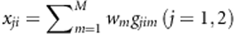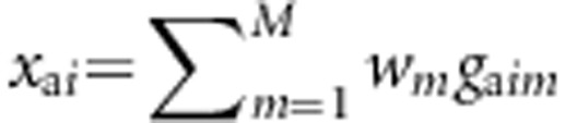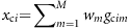Let , , and denote the combinations of genotypic scores at the M variants of the i^th sib-pair, the i^th case, and the i^th control, respectively, where w=(w₁,...,w_M) are weights and their values will be decided later. Denote the disease status of an individual by D with D=0 indicating a normal, whereas D=1 indicating a diseased individual.

The retrospective likelihood is given by

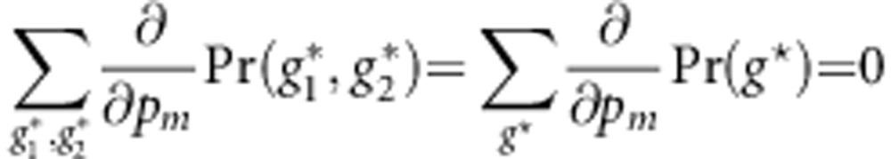
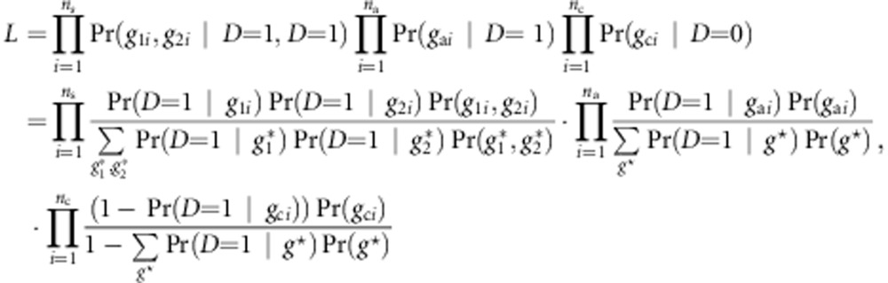where and represent all possible genotype pair for a sib-pair and g* represents all possible genotypes for an individual. Choose g₀=(0,…,0) as a baseline genotype. Let r(g) be the relative risk of genotype g to the baseline genotype. Following Schaid,³⁰ we use a log-linear model to model the relative risk, ie, r(g)=e^xβ, with x representing the combination of genotypic scores of the genotype g. Denote the risk of an individual with the baseline genotype as Pr(D=1|g₀)=e^α. Then, the retrospective likelihood is given by

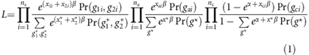where and represent the combinations of genotypic scores of the genotypes and , respectively, and x* represents the combination of genotypic scores of the genotype g*.

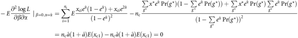
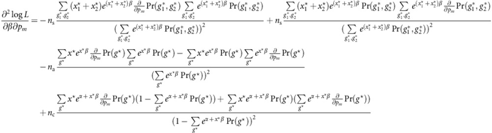
In Appendix A, we have shown that, under the assumption that the M variants are independent (our proposed test is still valid if this assumption is not true), the score test statistic to test the null hypothesis H₀:β=0 is given by

where , , and â are the maximum likelihood estimates (MLEs) of p_m and 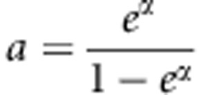under the null hypothesis, p_m is the MAF at the m^th variant, and . Under the null hypothesis, the likelihood function becomes

Based on L₀, has no explicit expression. Using the joint distribution of genotypes of a sib-pair given by Table 1, we can construct an expectation-maximization algorithm to calculate (see Appendix B). We cannot estimate α based on L₀, because L₀ does not contain α. We propose to estimate α based on the full likelihood function

Table 1. The joint distribution of genotypes of a sib-pair.

	Pr(g1, g2|IBD=0)				Pr(g1, g2|IBD=1)
g1/g2	0	1	2	g1/g2	0	1	2
0	q4	2pq3	p2q2	0	q3	pq2	0
1	2pq3	4p2q2	2p3q	1	pq2	pq	p2q
2	p2q2	2p3q	p4	2	0	p2q	p3

	Pr(g1, g2|IBD=2)		Pr(g1, g2)
g1/g2	0	1	2	g1/g2	0	1	2
0	q2	0	0	0	q2(1+q)2/4	pq2(q+1)/2	p2q2/4
1	0	2pq	0	1	pq2(q+1)/2	pq(pq+1)	p2q(p+1)/2
2	0	0	p2	2	p2q2/4	p2q(p+1)/2	p2(1+p)2/4

Notes: g1 and g2 are the genotypes of a sib-pair at a single variant. IBD means identical by decent. p and q are the allele frequencies of the two alleles.

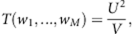
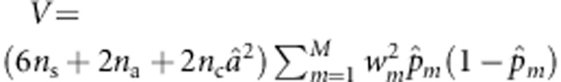
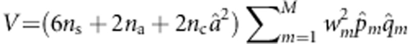
Based on L_full, the MLE of under the null hypothesis is . Using this estimate of a, U can be written as . Let , N=6n_s+2n_a+2n_câ², , and w=(w₁,…,w_M)^T. Then,

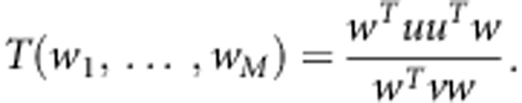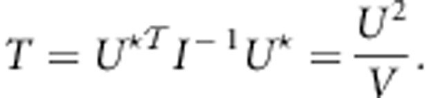
T(w₁,…,w_M) reaches its maxim when w=v⁻¹u. We define the statistic of the test for Testing the effect of an Optimally Weighted combination of variants for sib-pair data (TOW-sib) as

We use a special permutation test to evaluate P-values of TOW-sib. For each permutation, we have the following steps: (1) permute the multi-variant genotypes and get the permuted genotypes . (2) In the i^th sib-pair, given , we generate variant by variant according to the conditional distribution Pr(g₂|g₁) from Table 1. (3) Calculate , the value of T_TOW−sib based on the permuted genotypes , , and . We generate under the assumption that the M variants are independent. When the M variants are in linkage disequilibrium (LD), T_TOW−sib and may have different variances, although they have the same mean. In order to make T_TOW−sib and 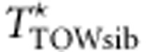have the same mean and same variance, we standardize T_TOW−sib such that T_{TOW−sib−ST}=(T_TOW−sib−μ_TOW−sib)/σ_TOW−sib, where μ_TOW−sib and are the estimates of the mean and variance of T_TOW−sib (see Appendix C on how to calculate μ_TOW−sib and ). Suppose we perform B times of permutations. Let denote the value of T_{TOW−sib−ST} based on data of the b^th permutation (b=0 denotes the original data). Then, the P-value of the test is given by .

For a simulation study with R replicates, the above procedure will be rather computationally expensive. In our simulation studies, we use the pooling permutation method proposed by Guo and Lin to evaluate P-values.³¹ In the pooling permutation method, permuted samples from all the replicates are pooled together to form a joint sample from the null distribution. Suppose that we have R replicates and we perform B permutations for each replicate. Let T_{TOW−sib−ST}^(b,r) denote the value of T_{TOW−sib−ST} based on data of the b^th permutation of the r^th replicate (b=0 denotes the original data). Then, the P-value of the test in the r^th replicate is given by

As the permutation samples are pooled across all replicates to form a sample from the null, B can be set to be much smaller than the situation when only one sample is analyzed.

We compare the performance of the proposed method with three existing methods: WSS,¹² sibpair-based weighted sum statistic (SPWSS),²⁸ and TOW.¹⁷ WSS and TOW are based on unrelated cases and controls, whereas SPWSS is based on affected sib-pairs, unrelated cases, and unrelated controls.

Simulation

The empirical Mini-Exome genotype data provided by the genetic analysis workshop 17 are used for simulation studies. This data set contains genotypes of 697 unrelated individuals on 3205 genes. The genotypes of the genetic analysis workshop 17 data set are extracted from the sequence alignment files provided by the 1000 Genomes Project for their pilot3 study (http://www.1000genomes.org). We choose four genes: ELAVL4 (gene1), MSH4 (gene2), PDE4B (gene3), and ADAMTS4 (gene4) with 10, 20, 30, and 40 variants, respectively. We merge the four genes to form a super gene (Sgene) with 100 variants with 86 rare variants (MAF<0.01) and 14 common variants (MAF≥0.01). We choose Sgene because the distributions of MAFs in the 100 variants in Sgene and in the 24 487 variants in all the 3205 genes are very similar.¹⁷ In our simulation studies, we generate genotypes based on the genotypes of 697 individuals in Sgene. We use the program fastPHASE to infer haplotypic phase for the 697 individuals and calculate haplotype frequencies.³² To generate the genotype of an individual, we generate two haplotypes according to the haplotype frequencies. To obtain the genotypes of a family, we first generate genotypes of parents. Then the genotypes of children are generated from parental haplotypes by random transmission. To generate a qualitative disease affection status, we use a liability threshold model based on a continuous phenotype (quantitative trait). An individual is defined to be affected if the individual's phenotype is at least one standard deviation larger than the phenotypic mean. This yields a prevalence of 16% for the simulated disease in the general population. In the following, we describe how to generate a quantitative trait.

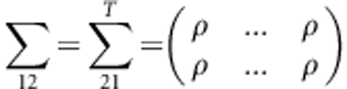
Under the null hypothesis, we generate trait values for unrelated individuals according to the standard normal distribution. For a family with m children, let Y₁=(y_F,y_M) and Y₂=(y₁,y₂,⋯,y_m) denote the trait values of the parents and the m children in a family, respectively. Assume that (Y₁,Y₂) follows a multivariate normal distribution with a mean vector of zero and variance-covariance matrix of, where , , and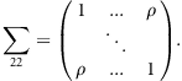

This variance-covariance matrix indicates that the parents in each family are independent, and the correlation coefficient between a parent and a child or between two children is constant, ρ (in this study, ρ=0.2). To generate trait values of all members in each family, we first generate the trait value of a parent by using a standard normal distribution. Then, trait values of the children are generated by a normal distribution with a mean vector 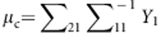and a variance–covariance matrix .

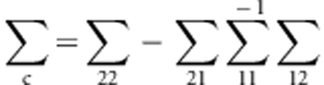Under the alternative hypothesis, we choose n_cau rare variants (MAF<1%) as causal variants. The value of n_cau is determined by p_cau, the percentage of causal variants in rare variants. Let pp denote the percentage of protective variants in causal variants, then the number of protective variants and the number of risk variants are n_p=n_cau·pp and n_r=n_cau·(1−pp), respectively. For the j^th member in the i^th family, let and denote the genotypic scores of the risk variant and the protective variant, respectively. Assume that all causal variants have the same heritability. Then the disease model is given by , where and are coefficients and their values depend on the total heritability, and ɛ_ij is the trait value under the null hypothesis.

To generate affected sib-pairs, we generate families with two children. We keep generating families with two children until we have generated enough families with two affected children.

Results

In simulation studies, P-values are estimated using a pooling permutation method in which permuted samples from all the replicates are pooled together to form a joint sample from the null distribution.³¹ In each replicate, we perform 20 permutations. Type I error rates are evaluated using 10 000 replicated samples, whereas powers are evaluated using 500 replicated samples.

For type I error evaluation, we consider different haplotype structures (different genes), different sample sizes, different designs, and different significance levels. For 10 000 replicated samples, the 95% confidence intervals for type I error rates of nominal levels 0.05, 0.01, and 0.001 are (0.046, 0.054), (0.008, 0.012), and (0.0004, 0.0016), respectively. The estimated type I error rates of the proposed test are summarized in Tables 2 and 3. As shown by these tables, all the estimated type I error rates are within the 95% confidence intervals, which indicates that the proposed test is valid.

Table 2. Estimated type I error rates of TOW-sib for the design of affected sib-pairs and unrelated controls based on 10 000 replicated samples.

	Significance level=0.05			Significance level=0.01			Significance level=0.001
	Sample size			Sample size			Sample size
	1000	2000	4000	1000	2000	4000	1000	2000	4000
Gene 1	0.0467	0.0492	0.0472	0.0108	0.0094	0.0098	0.0014	0.0016	0.0012
Gene 2	0.0469	0.0477	0.0524	0.0086	0.0085	0.0119	0.0008	0.0008	0.0014
Gene 3	0.0469	0.0484	0.0468	0.0094	0.0113	0.0083	0.0013	0.0014	0.0007
Gene 4	0.0479	0.0478	0.0491	0.0088	0.0096	0.0092	0.0007	0.0013	0.0010
Sgene	0.0465	0.0467	0.0478	0.0091	0.0086	0.0088	0.0008	0.0008	0.0008

Note: n_sample is the sample size, ie, the total number of individuals in the sample. n_sib is the number of affected sib-pairs. n_case is the number of unrelated cases. n_control is the number of unrelated controls. n_sib = n_sample/4, n_case=0, and n_control=n_sample/2.

Table 3. Estimated type I error rates of TOW-sib for the design of affected sib-pairs, unrelated cases, and unrelated controls based on 10 000 replicated samples.

	Significance level=0.05			Significance level=0.01			Significance level=0.001
	Sample size			Sample size			Sample size
	1000	2000	4000	1000	2000	4000	1000	2000	4000
Gene 1	0.0467	0.0507	0.0512	0.0108	0.0118	0.0091	0.0014	0.0014	0.0011
Gene 2	0.0479	0.0534	0.0529	0.0086	0.0103	0.0112	0.0008	0.0011	0.0015
Gene 3	0.0469	0.0521	0.0537	0.0094	0.0108	0.011	0.0013	0.0015	0.0014
Gene 4	0.0469	0.0539	0.0526	0.0088	0.0104	0.0112	0.0007	0.0014	0.0013
Sgene	0.0465	0.0521	0.0516	0.0091	0.0118	0.0117	0.0008	0.0014	0.0015

Note: n_sample is sample size, ie, the total number of individuals in the sample. n_sib is the number of affected sib-pairs. n_case is the number of unrelated cases. n_control is the number of unrelated controls. n_sib=n_sample/8, n_case=n_sample/4, and n_control=n_sample/2.

For fixed number of total cases and fixed number of total individuals, power comparisons for power as a function of the number of affected sib-pairs are given in Figure 1. As shown by Figure 1, the power of TOW-sib increases with the increase of the number of affected sib-pairs. With the increase of the number of affected sib-pairs, the power of SPWSS increases if the number of affected sib-pairs is less than 20% of total number of cases and the power of SPWSS decreases otherwise. Therefore, in the following discussion, the number of affected sib-pairs is equal to the half of total number of cases in the design for TOW-sib and the number of affected sib-pairs is equal to 20% of total number of cases in the design for SPWSS. The powers of TOW and WSS do not have relation with the number of affected sib-pairs. In almost all the cases, TOW-sib is the most powerful test. When the percentage of causal variants is small (10%), SPWSS is more powerful than TOW and WSS if the number of affected sib-pairs is between 10 and 45% of the total number of cases. When the percentage of causal variants is large (50%), SPWSS is the least powerful test.

Figure 1.

Power comparisons of four tests for power as a function of number of affected sib-pairs. TOW and WSS are based on 1000 unrelated cases and 1000 unrelated controls. For TOW-sib and SPWSS, the sample size is 2000, where number of unrelated controls is 1000 and number of unrelated cases plus twice of the number of affected sib-pairs is 1000. Total heritability is 0.03. pcau denotes the percentage of causal variants in rare variants; pp denotes the percentage of protective variants in causal variants. The power is evaluated at a significance level of 0.001.

As shown by power comparisons for power as a function of heritability and for power as a function of the percentage of protective variants (Figures 2 and 3), TOW-sib is the most powerful test in all the cases. When the percentage of causal variants is small (10%), SPWSS is more powerful than TOW and WSS. When the percentage of causal variants is large (50%), SPWSS and TOW have similar power and are less powerful than WSS if the percentage of protective variants is small and are more powerful than WSS if the percentage of protective variants is large.

Figure 2.

Powers as a function of heritability. TOW and WSS are based on 1000 unrelated cases and 1000 unrelated controls. SPWSS is based on 1000 unrelated controls, 600 unrelated cases, and 200 affected sib-pairs. TOW-sib is based on 1000 unrelated controls and 500 affected sib-pairs. pcau denotes the percentage of causal variants in rare variants; pp denotes the percentage of protective variants in causal variants. The power is evaluated at a significance level of 0.001.

Figure 3.

Powers as a function of percentage of protective variants. TOW and WSS are based on 1000 unrelated cases and 1000 unrelated controls. SPWSS is based on 1000 unrelated controls, 600 unrelated cases, and 200 affected sib-pairs. TOW-sib is based on 1000 unrelated controls and 500 affected sib-pairs. pcau denotes the percentage of causal variants in rare variants; herit denotes the total heritability. The power is evaluated at a significance level of 0.001.

Figure 4 shows power comparisons for power as a function of the percentage of causal variants. This figure shows that TOW-sib is the most powerful test in all the cases and the power of TOW-sib is not affected much by the percentage of causal variants. With the increase of the percentage of causal variants, the powers of WSS and TOW increase, whereas the power of SPWSS decreases. It is easy to understand that the power increases with the increase of the percentage of causal variants because larger percentage of causal variants or smaller percentage of neutral variants means smaller noise level. The reason of decrease in power of SPWSS with the increase of the percentage of causal variants probably is that it is easier to estimate weights when the percentage of causal variants is smaller. We also conduct a set of simulations to compare the powers for different values of ρ. The results (Supplementary Figure 1) show that the power comparisons have similar patterns for different values of ρ.

Figure 4.

Powers as a function of percentage of causal variants. TOW and WSS are based on 1000 unrelated cases and 1000 unrelated controls. SPWSS is based on 1000 unrelated controls, 600 unrelated cases, and 200 affected sib-pairs. TOW-sib is based on 1000 unrelated controls and 500 affected sib-pairs. pp denotes the percentage of protective variants in causal variants; herit denotes the total heritability. The power is evaluated at a significance level of 0.001.

In summary, TOW-sib is the most powerful test in all the cases. Among other three tests: WSS, SPWSS, and TOW, none is consistently more powerful than the other two.

Discussion

There is increasing interest to detect associations between rare variants and complex traits. Recently, several statistical methods for detecting rare variant associations by jointly considering multiple variants in a genomic region have been developed for unrelated individuals. However, statistical methods for detecting rare variant associations under family-based designs have not received as much attention as methods for unrelated individuals, although family-based designs have been shown to improve power to detect rare variants.^{28, 29} Motivated by the facts that rare disease variants will be enriched in family data³³ and a large number of affected sib-pairs for a variety of diseases has been collected by traditional linkage studies, we develop TOW-sib to detect associations between the optimal combination of rare variants in a genomic region and complex traits based on affected sib-pairs and unrelated individuals. TOW-sib is robust to the directions of the effects of causal variants and is also relatively robust to the number of neutral variants. The proposed method does not require a MAF filtering threshold and can be applied to genomic regions that contain both rare and common variants. Our simulations demonstrated that TOW-sib using affected sib-pairs can be dramatically more powerful than the methods based on unrelated individuals and the existing methods based on affected sib-pairs.

Although TOW-sib is derived under the assumption that variants are independent, our simulation results show that TOW-sib is still a valid test when variants are in LD. Our simulations for type I error evaluation are based on the LD structures of genes 1–4 and, in each gene, there are variants in strong LD (Supplementary Tables 1–4). The correct type I error rates of TOW-sib in our simulations (Tables 2 and 3) indicate that this test is valid even if variants are in LD.

The current version of TOW-sib cannot adjust for covariates. It is possible to extend TOW-sib to be able to adjust for covariates. Denote z_ji, z_ai, and z_ci as the covariates of the j^th individual in the i^th sib-pair, the i^th cases, and the i^th controls, respectively. With covariates, the retrospective likelihood can be written as

Let 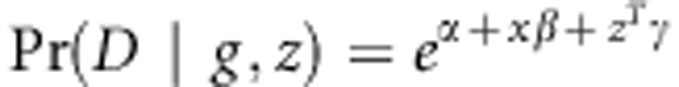, where x represents the combination of genotypic scores of the genotype g and z denotes covariates. Based on this likelihood, we can derive a score test statistic. However, the details of adjusting for covariates in TOW-sib need further investigation.

TOW-sib uses the optimal data-driven weights. TOW-sib belongs to quadratic tests and thus is robust to the directions of the effects of causal variants. We can use other weights. For example, in the score test statistic T(w₁,…,w_M), we can use the weights suggested by Madsen and Browning,¹² that is, , where p_m is the estimated MAF with pseudo-counts at the m^th variant. We call the score test T(w₁,…,w_M) with 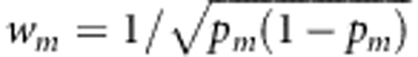WSS-sib. WSS-sib belongs to burden tests. When most of the rare variants are causal and the directions of the effects of causal variants are all the same, WSS-sib can outperform TOW-sib; otherwise, TOW-sib should outperform WSS-sib. To increase the robustness of the tests, we can also construct combined tests by combining information from TOW-sib and WSS-sib. One thing we want to make clear is the term ‘optimal weight'. The optimal weight in this paper only means that the selected weight makes the score test statistic maximum, it does not mean that the selected weight makes the score test to have the maximum power.

In this study, we estimate based on the full likelihood. We can also use other estimates of a. Different estimates do not affect type I error, but do affect power. Our simulations (results not shown) show that the MLE of a based on the full likelihood is a good choice. We compare our proposed method with two methods based on the case/control design to see if the affected sib-pair design is more powerful than the case/control design. This is our main purpose. We also compare our proposed method with one of the existing methods that are applicable to the affected sib-pair design. Although several methods^{28, 29} developed recently are applicable to the affected sib-pair design, we only choose SPWSS²⁸ to compare with because SPWSS is most relevant to our proposed method.

Appendix A

Score Test Statistic

Using notations in the Method section, from Equation (1), the log retrospective likelihood is given by

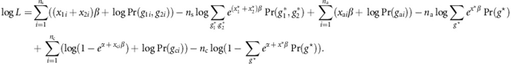Then,

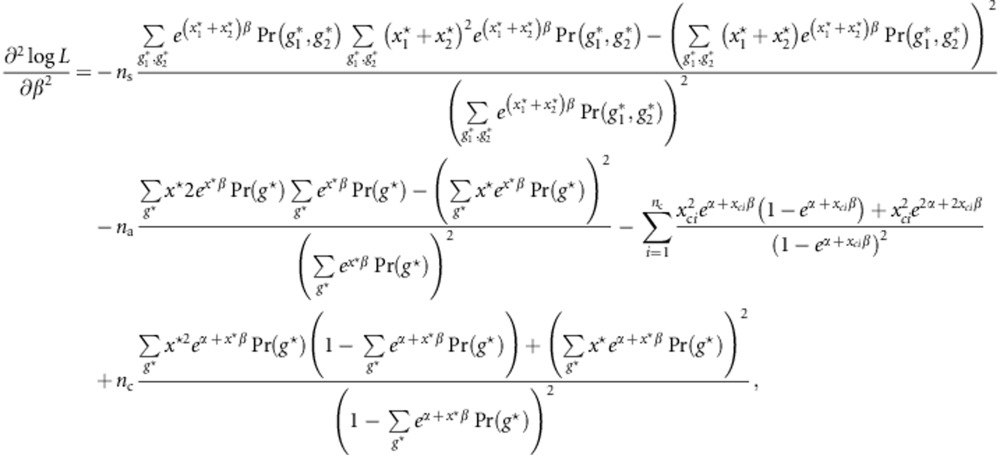Let P=(p₁,…,p_M)^T and . Note that and

for m=1,…,M. We have

and

Similarly, we have

Let , , U*=(U,0,0)^T denote the score vector, and I denote the information matrix. Then, the score test statistic is given by

Appendix B

Expectation-maximization Algorithm to Estimate Allele Frequency Based on Sib-pairs and Unrelated Individuals

Consider a variant with two alleles. Let B denote the minor allele and p denote the frequency of allele B. We use the following notations.

N: the number of unrelated individuals

N_f: the number of sib-pairs

n: the number of minor alleles in genotypes of the N unrelated individuals

n_ij: the number of sib-pairs with genotype pair (i,j) or (j,i)

: the number of sib-pairs with genotype pair (i,j) or (j,i) and the pair of genotypes has k alleles IBD E-step:

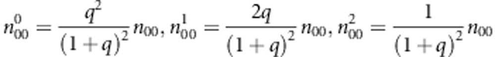
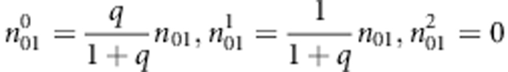
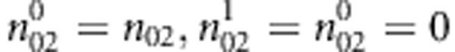
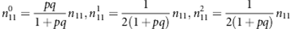
M-step: where

Appendix C

Mean and Variance of TOW-sib

It is easy to know that . In the following, we will calculate the variance of T_TOW−sib.

Let g₁ and g₂ denote genotypes of a sib-pair, x=g₁+g₂, and p (q=1−p) denote the MAF. Using the distribution given by Table 1, we have

E(g₁−2p)⁴=2pq, var(x)=6 pq, and E(x−4p)⁴=6pq(pq+3).

We know that , , and 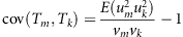. Let n=n_s+n_a+n_c, x_i=g_1im+g_2im−4p_m for i=1,…,n_s, 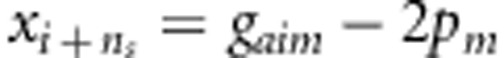for i=1,…,n_a, for i=1,…,n_c, and y_i is similarly defined for the k^th variant as x_i for the m^th variant.

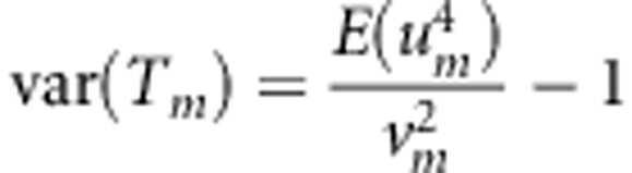
We can calculate the variance of T_TOW−sib if we note that

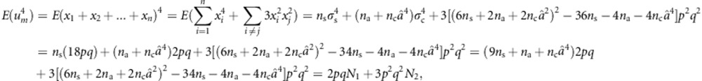where N₁=9n_s+n_a+n_câ⁴, N₂=(6n_s+2n_a+2n_câ²)²−34n_s−4n_a−4n_câ⁴, and ;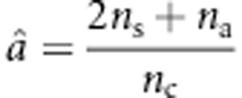

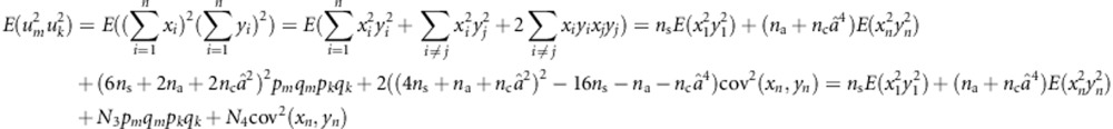where N₃=(6n_s+2n_a+2n_câ²)², N₄=2((4n_s+n_a+n_câ²)²), E(x₁²y₁²) is estimated with 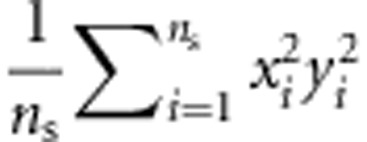, E(x_n²y_n²) is estimated with 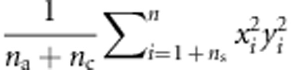, and cov(x_n, y_n) is estimated with .

The authors declare no conflict of interest.

References

- McCarthy MI, Abecasis GR, Cardon LR, et al. Genome-wide association studies for complex traits: consensus, uncertainty and challenges. Nat Rev Genet. 2008;9:356–369. doi: 10.1038/nrg2344. [DOI] [PubMed] [Google Scholar]
- Manolio TA, Collins FS, Cox NJ, et al. Finding the missing heritability of complex diseases. Nature. 2009;461:747–753. doi: 10.1038/nature08494. [DOI] [PMC free article] [PubMed] [Google Scholar]
- Marini NJ, Gin J, Ziegle J, et al. The prevalence of folate-remedial MTHFR enzyme variants in humans. Proc Natl Acad Sci USA. 2008;105:8055–8060. doi: 10.1073/pnas.0802813105. [DOI] [PMC free article] [PubMed] [Google Scholar]
- Ji W, Foo JN, O'Roak BJ, et al. Rare independent mutations in renal salt handling genes contribute to blood pressure variation. Nat Genet. 2008;40:592–599. doi: 10.1038/ng.118. [DOI] [PMC free article] [PubMed] [Google Scholar]
- Cohen JC, Pertsemlidis A, Fahmi S, et al. Multiple rare variants in NPC1L1 associated with reduced sterol absorption and plasma lowdensity lipoprotein levels. Proc Natl Acad Sci USA. 2006;103:1810–1815. doi: 10.1073/pnas.0508483103. [DOI] [PMC free article] [PubMed] [Google Scholar]
- Nejentsev S, Walker N, Riches D, Egholm M, Todd JA. Rare variants of IFIH1, a gene implicated in antiviral responses, protect against type 1 diabetes. Science. 2009;324:387–389. doi: 10.1126/science.1167728. [DOI] [PMC free article] [PubMed] [Google Scholar]
- Zhu X, Feng T, Li Y, Lu Q, Elston RC. Detecting rare variants for complex traits using family and unrelated data. Genet Epidemiol. 2010;34:171–187. doi: 10.1002/gepi.20449. [DOI] [PMC free article] [PubMed] [Google Scholar]
- Andrés AM, Clark AG, Shimmin L, Boerwinkle E, Sing CF, Hixson JE. Understanding the accuracy of statistical haplotype inference with sequence data of known phase. Genetic Epi. 2007;31:659–671. doi: 10.1002/gepi.20185. [DOI] [PMC free article] [PubMed] [Google Scholar]
- Metzker ML. Sequencing technologies – the next generation. Nat Rev Genet. 2010;11:31–46. doi: 10.1038/nrg2626. [DOI] [PubMed] [Google Scholar]
- Morgenthaler S, Thilly WG. A strategy to discover genes that carry multiallelic or mono-allelic risk for common diseases: a cohort allelic sums test (CAST) Mutat Res. 2007;615:28–56. doi: 10.1016/j.mrfmmm.2006.09.003. [DOI] [PubMed] [Google Scholar]
- Li B, Leal SM. Methods for detecting associations with rare variants for common diseases: application to analysis of sequence data. Am J Hum Genet. 2008;83:311–321. doi: 10.1016/j.ajhg.2008.06.024. [DOI] [PMC free article] [PubMed] [Google Scholar]
- Madsen BE, Browning SR. A groupwise association test for rare mutations using a weighted sum statistic. PLoS Genet. 2009;5:e1000384. doi: 10.1371/journal.pgen.1000384. [DOI] [PMC free article] [PubMed] [Google Scholar]
- Price AL, Kryukov GV, de Bakker PI, et al. Pooled association tests for rare variants in exon-resequencing studies. Am J Hum Genet. 2010;86:832–838. doi: 10.1016/j.ajhg.2010.04.005. [DOI] [PMC free article] [PubMed] [Google Scholar]
- Zawistowski M, Gopalakrishnan S, Ding J, Li Y, Grimm S, Zollner S. Extending rare-variant testing strategies: analysis of noncoding sequence and imputed genotypes. Am J Hum Genet. 2010;87:604–617. doi: 10.1016/j.ajhg.2010.10.012. [DOI] [PMC free article] [PubMed] [Google Scholar]
- Wu M, Lee S, Cai T, Li Y, Boehnke M, Lin X. Rare variant association testing for sequencing data using the sequence kernel association test (SKAT) Am J Hum Genet. 2011;89:82–93. doi: 10.1016/j.ajhg.2011.05.029. [DOI] [PMC free article] [PubMed] [Google Scholar]
- Lee S, Emond MJ, Bamshad MJ, et al. Optimal unified approach for rare-variant association testing with application to small-sample case-control whole-exome sequencing studies. Am J Hum Genet. 2012;91:224–237. doi: 10.1016/j.ajhg.2012.06.007. [DOI] [PMC free article] [PubMed] [Google Scholar]
- Sha Q, Wang X, Wang X, Zhang S. Detecting association of rare and common variants by testing an optimally weighted combination of variants. Genet Epidemiol. 2012;36:561–571. doi: 10.1002/gepi.21649. [DOI] [PubMed] [Google Scholar]
- Derkach A, Lawless J, Sun L. Robust and powerful tests for rare variants using Fisher's method to combine evidence of association from two or more complementary tests. Genetic Epi. 2012;37:110–121. doi: 10.1002/gepi.21689. [DOI] [PubMed] [Google Scholar]
- Neale BM, Rivas MA, Voight BF, et al. Testing for an unusual distribution of rare variants. PLoS Genet. 2011;7:e1001322. doi: 10.1371/journal.pgen.1001322. [DOI] [PMC free article] [PubMed] [Google Scholar]
- Han F, Pan W. A data-adaptive sum test for disease association with multiple common or rare variants. Hum Hered. 2010;70:42–54. doi: 10.1159/000288704. [DOI] [PMC free article] [PubMed] [Google Scholar]
- Hoffmann TJ, Marini NJ, Witte JS. Comprehensive approach to analyzing rare genetic variants. PLoS One. 2010;5:e13584. doi: 10.1371/journal.pone.0013584. [DOI] [PMC free article] [PubMed] [Google Scholar]
- Lin D-Y, Tang Z-Z. A general framework for detecting disease associations with rare variants i n sequencing studies. Am J Hum Genet. 2011;89:354–367. doi: 10.1016/j.ajhg.2011.07.015. [DOI] [PMC free article] [PubMed] [Google Scholar]
- Yi N, Zhi D. Bayesian analysis of rare variants in genetic association studies. Genet Epidemiol. 2011;35:57–69. doi: 10.1002/gepi.20554. [DOI] [PMC free article] [PubMed] [Google Scholar]
- Sha Q, Wang S, Zhang S. Adaptive clustering and adaptive weighting methods to detect disease associated rare variants. Eu J Hum Genet. 2013;21:332–337. doi: 10.1038/ejhg.2012.143. [DOI] [PMC free article] [PubMed] [Google Scholar]
- Shi G, Rao D. Optimum designs for next-generation sequencing to discover rare variants for common complex disease. Genetic Epidemiol. 2011;35:572–579. doi: 10.1002/gepi.20597. [DOI] [PMC free article] [PubMed] [Google Scholar]
- Fang S, Sha Q, Zhang S. Two adaptive weighting methods to test for rare variant associations in family-based designs. Genet Epidemiol. 2012;36:499–507. doi: 10.1002/gepi.21646. [DOI] [PubMed] [Google Scholar]
- Liu D, Leal S. A unified framework for detecting rare variant quantitative trait associations in pedigree and unrelated individuals via sequence data. Hum Hered. 2012;73:105–122. doi: 10.1159/000336293. [DOI] [PMC free article] [PubMed] [Google Scholar]
- Feng T, Elston R, Zhu X. Detecting rare and common variants for complex traits: sibpair and odds ratio weighted sum statistics (SPWSS, ORWSS) Genet Epidemiol. 2011;35:398–409. doi: 10.1002/gepi.20588. [DOI] [PMC free article] [PubMed] [Google Scholar]
- Zhu Y, Xiong M. Family-based association studies for next-generation sequencing. Am J Hum Genet. 2012;90:1028–1045. doi: 10.1016/j.ajhg.2012.04.022. [DOI] [PMC free article] [PubMed] [Google Scholar]
- Schaid DJ. General score tests for associations of genetic markers with disease using cases and their parents. Genet Epidemiol. 1996;13:423–449. doi: 10.1002/(SICI)1098-2272(1996)13:5<423::AID-GEPI1>3.0.CO;2-3. [DOI] [PubMed] [Google Scholar]
- Guo W, Lin S. Generalized linear modeling with regularization for detecting common disease rare haplotype association. Genet Epidemiol. 2009;33:308–316. doi: 10.1002/gepi.20382. [DOI] [PMC free article] [PubMed] [Google Scholar]
- Scheet P, Stephens M. A fast and flexible statistical model for large-scale population genotype data: applications to inferring missing genotypes and haplotypic phase. Am J Hum Genet. 2006;78:629–644. doi: 10.1086/502802. [DOI] [PMC free article] [PubMed] [Google Scholar]
- Feng T, Zhu X. Genome-wide searching of rare genetic variants in WTCCC data. Hum Genet. 2010;128:269–280. doi: 10.1007/s00439-010-0849-9. [DOI] [PMC free article] [PubMed] [Google Scholar]
Associated Data
This section collects any data citations, data availability statements, or supplementary materials included in this article.