Significance
Large and complex macromolecular assemblies—like RNA and DNA polymerases, the kinetochore, the ribosome, ATP synthase, and many others—are critical components of the cell. To fully characterize these molecular machines, it is not sufficient to rely solely on traditional structural methods, like cryo-EM and X-ray crystallography that provide great structural detail in vitro; we need experimental and theoretical tools that can describe the organization of these machines in their native cellular environment so as to better understand their function. Here we provide a strategy for extracting precisely this information directly from superresolution imaging data, a state-of-the-art technique for probing biological structures in living cells below the diffraction limit.
Keywords: single molecule, fluorescence, protein complexes, superresolution, counting problem
Abstract
Superresolution imaging methods—now widely used to characterize biological structures below the diffraction limit—are poised to reveal in quantitative detail the stoichiometry of protein complexes in living cells. In practice, the photophysical properties of the fluorophores used as tags in superresolution methods have posed a severe theoretical challenge toward achieving this goal. Here we develop a stochastic approach to enumerate fluorophores in a diffraction-limited area measured by superresolution microscopy. The method is a generalization of aggregated Markov methods developed in the ion channel literature for studying gating dynamics. We show that the method accurately and precisely enumerates fluorophores in simulated data while simultaneously determining the kinetic rates that govern the stochastic photophysics of the fluorophores to improve the prediction’s accuracy. This stochastic method overcomes several critical limitations of temporal thresholding methods.
Protein–protein and protein–nucleic acid interactions are responsible for most of information processing and control in the cell. Moreover, essential cellular tasks such as replication, transcription, translation, recombination, control of gene expression, and transport of proteins across membranes, to cite a few, all depend on the interaction among preorganized molecular assemblies (1–4). Developing a mechanistic understanding of cell biology requires a quantitative determination of macromolecular organization and interaction in living cells. In particular, characterizing protein–protein and protein–nucleic acid complexes and their stoichiometric ratios is a first step in determining how altered stoichiometries may lead to disease states of the cell (5–8).
Conventional optical microscopy is diffraction limited and typically cannot resolve images below the 250-nm range, but superresolution (SR) methods can achieve tens of nanometer resolution (9–12). One such SR method is photoactivated localization microscopy (PALM), where temporal separation is achieved by illuminating a sample with inactive (i.e., nonfluorescing) fluorophores under low light intensity. The light stochastically triggers fluorophore activation. Once active, a fluorophore is excited by light of a different wavelength and releases a burst of photons (an emission burst). This emission is used to locate the position of the emitter with uncertainty that depends only on the number of photons detected. A short time later, the fluorophore irreversibly photobleaches. The low probability of photoactivation ensures that two fluorophores separated less than the diffraction limit will most probably not emit simultaneously. In this manner, the PALM fluorophores that could not otherwise be spatially separated are instead separated in time. The fluorophores in PALM are genetically encoded with photoactivatable fluorescent proteins (PA-FPs) (13)—often mEos2 (14) or Dendra2 (15, 16)—that are fused to proteins of interest.
Generating PALM images is now routine, and both SR tagging techniques and instrumentation have progressed much faster than our ability to analyze PALM images. In particular, extracting protein complex stoichiometry information from PALM data is not straightforward. Rather, stoichiometry is often determined using in vitro (e.g., coimmunoprecipitation) (17) or coarser (diffraction-limited) methods (18–23). However, PALM has the potential to provide molecular counting with single molecule sensitivity and in vivo. However, several obstacles remain: (i) PA-FP “blinking” leads to severe overcounting biases. Blinking refers to a process by which a PA-FP produces a series of intermittent emission bursts, instead of a single continuous burst (24, 25), by transiently transitioning to a “dark” state. Accordingly, counting the number of emission bursts over a region of interest (ROI) will lead to overestimating the number of labeled molecules; and (ii) Unknown blinking statistics. Often the blinking properties of common PA-FPs are known in vitro, but not in vivo in the specific cellular compartment occupied by the molecules. Characterizing the blinking properties of PA-FPs in their cellular context is required because these properties are highly sensitive to their local cellular environment (pH, ionic strength) (26–33). An analytical method capable of extracting the blinking statistics of PA-FPs inside the cell to correct for blinking is not available.
Here, we describe a stochastic approach for dealing with these obstacles. Our approach is an adaptation of the continuous time aggregated Markov model (AMM) techniques developed in the ion channel literature to estimate kinetic rates using maximum-likelihood methods for channel opening and closing events in patch-clamp experiments (34–38). Our objective is, thus, to arrive at molecular quantification in PALM. Previous studies have addressed the PALM counting problem by setting a temporal threshold (39–42). In those studies, a pair of emission bursts separated by a time shorter than some are grouped together and assigned to a single PA-FP. Bursts separated by a time longer than are considered to be from separate PA-FPs. Our method overcomes several important limitations of temporal thresholding methods because it treats the properties of PA-FPs stochastically. First, by contrast to temporal thresholding methods that necessitate advance knowledge of kinetic rates to determine the optimal value of , our method does not require knowledge of kinetic rates beforehand. Kinetic rates are an output of the method, not an input. Second, the method is not tied to a specific kinetic model. We can easily explore alternative kinetic models, such as those with multiple blinking states or with time-varying rates. Third, we can correct for missed transitions which occur if typical PA-FP fluorescence times are as fast as or faster than the frame integration time. Finally, we can use fluorescence intensities (which can vary if multiple PA-FPs fluoresce at once) to inform our estimate for the complex stoichiometry.
In what follows we develop the theoretical methodology and benchmark the method on sample data as well as on synthetic data. We will describe how it is possible to derive from SR data not only the number of PA-FPs, as well as their photophysics, but also determine error bars around all of the estimates.
Results
Analysis of Simulated Data.
Consider the model shown in Fig. 1 for the photophysics of a single PA-FP. There are four possible states: inactive (I), active (A), dark (D), or photobleached (B). Once active, the PA-FP has two options: (i) it can blink possibly transitioning multiple times between the active and the dark state or (ii) it can irreversibly photobleach. Fluorescence is only detected from the active state, not in the other three states. Now consider a collection of N identical PA-FPs, each of which is governed by the model of Fig. 1.
Fig. 1.
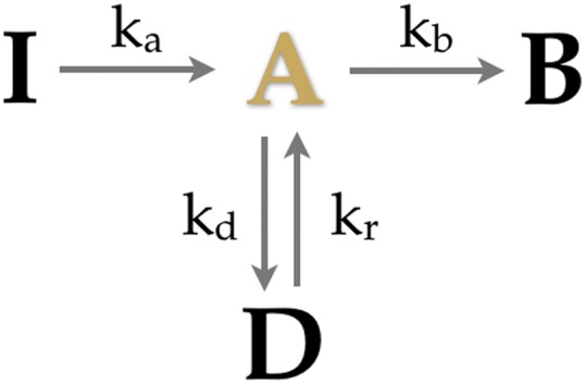
Kinetic model for PA-FP blinking. This kinetic model has four states inactive (I), active (A), dark (D), and photobleached (B). The only fluorescent state is A. We name the transitions between states this way: activation , blinking , recovery , and photobleaching .
Thresholding methods used in enumerating PA-FPs do not treat the stochastic nature of the fluorescence bursts explicitly. Thus, these methods cannot separate overlapping PA-FP signals where one FP activates before the last FP has photobleached. These methods also cannot treat superposing signals, which occur when two or more FPs fluoresce at the same time. Overlapping and superposing signals arise when multiple PA-FP spikes occur over a short period. This can happen when (i) there are a large number of PA-FPs; (ii) the PA-FP blinking rate is fast and the PA-FP photobleaching rate is slow; and (iii) the PA-FP photoactivation rate is fast and the PA-FP photobleaching rate is slow.
Without a priori knowing the PA-FP number, N, or the PA-FP’s properties, it is not possible to ascertain whether overlapping and superposing signals are improbable. Thus, in these conditions, if the problem at hand is specifically to determine N, the use of thresholding methods may not be appropriate. The method developed here, by contrast, is applicable for any N and PA-FP, regardless of its photophysical properties (activation, blinking, and photobleaching) because it explicitly treats them as the stochastic events they are.
To benchmark our method for finding kinetic rates and N from the data, we first analyzed 200 simulated trajectories, each one representing a collection of PA-FPs.
These simulated trajectories (a sample of which is shown in Fig. S1) were generated using the Gillespie stochastic simulation algorithm (43). That is, the PA-FP photophysical dynamics were simulated stochastically according to the model given in Fig. 1 and the time trace recorded a fluorescence signal only during times in which any of the PA-FPs were in the A state.
There are several assumptions that these simulations make:
-
i)
We assume that we have a unique dark and active state. If the number of dark and active states is greater than one, we will find that our estimates for the rates will come with large error bars (we will later see this for the case of Dendra2) and, in this case, additional information must be provided to specify the number of states needed.
-
ii)
We assume that the breadth of the distribution over N for our simulated data arises only from finite data. In reality, finite data provides a lower bound on the breadth of the distribution over N. The remainder of the distribution’s breadth arises from the intrinsic variability in the stoichiometry of the complex which we will discuss later.
-
iii)
We assume all PA-FPs photoactivate. Recent work suggests that the photoactivation efficiency ranges from only 40–60% depending on the PA-FP (44); to correct for this, we would amend our PA-FP topology to add another state to which state I can irreversibly transition without ever entering state A.
-
iv)
We assume that maturation of all PA-FPs (mEos2 and Dendra2) used in the in vitro experiments is complete; we assume this because the elapsed time—from protein expression to the point where purified protein are obtained—is longer than the maturation half-time (90 and 120 min for Dendra2 and mEos2, respectively) (45, 46).
-
v)
We assume that protein complexes are well separated in space, which is often the case in experiments. For instance, the bacterial flagellar motor complex—with ∼22 MotB monomers forming part of each complex—are spatially well separated (20), as are individual kinetochores associated with six or more proteins linking kinetochore microtubules to centromeric DNA (47). For the complicated case where complexes are closely packed (i.e., packed within region spatially nonresolvable by PALM), our analysis should yield a distribution over N peaked at multiples of some number, e.g., N = 5; this, in itself, is important information that would then motivate future experiments in an effort to establish whether complexes aggregate or coincidentally colocalize within an ROI.
We simulated three different blinking scenarios: moderate blinking (set 1), fast blinking (set 2), and slow blinking (set 3). We generated 200 synthetic traces for each scenario. The parameters for the three sets are summarized in Table 1. We tuned the ratio between the blinking rate and the photobleaching rate to control the blinking behavior. If is large, relative to , then many blinking events will occur before photobleaching. If is much smaller than , the PA-FP is more likely to photobleach without blinking.
Table 1.
Transition rates for simulated data
| Rate constant | Set 1 | Set 2 | Set 3 |
| 0.5 | 0.5 | 0.5 | |
| 3.0 | 10.0 | 0.1 | |
| 0.1 | 0.1 | 0.1 | |
| 1.0 | 1.0 | 1.0 | |
| 3 | 10 | 0.1 |
Kinetic rates used to generate simulated data sets. Rates in units of Hz.
To find the model parameters from the synthetic data, we use a maximum-likelihood procedure detailed in Materials and Methods. The likelihood function is based on the likelihood of observing a particular on-off fluorescence time trace in the data, which is then maximized with respect to the model parameters.
In the analysis of these data sets, we used a bootstrapping approach (resampling data with replacement) to determine the precision of our parameter estimates (48, 49). We randomly selected a subset of trajectories and determined the rates that maximized the sum of the log-likelihoods of the selected trajectories. We constructed a distribution of rates by repeating this process (200 times) for other randomly selected sets of trajectories. Our estimate for each parameter is the mean of the corresponding distribution, and we compute the 95% confidence interval based on percentiles of the distribution. The results are shown in Figs. 2 and 3 (for data set 1 and 2) and Fig. S2 (for data set 3).
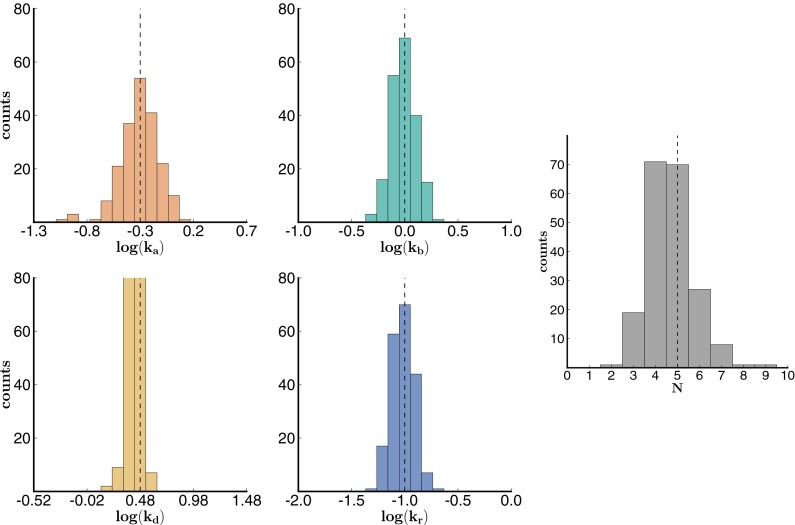
Fig. 2.
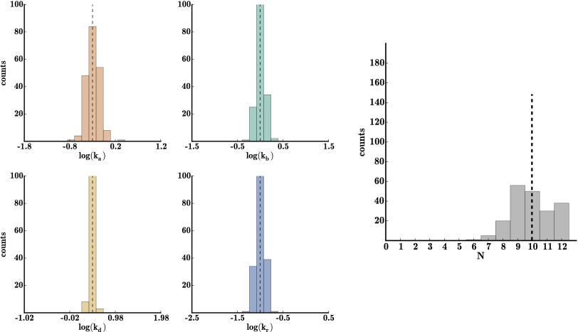
Histogram of bootstrapping results from simulated data set 1. Histogram of bootstrapping results from simulated data set 1 with 200 traces (200 bootstrap iterations). The theoretically expected results are shown in the dotted line.
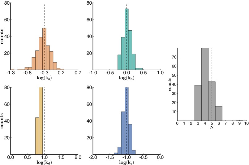
Fig. 3.
Histogram of bootstrapping results from simulated data set 2. Histogram of bootstrapping results from simulated data set 2 with 200 traces (200 bootstrap iterations). An overall bias toward slow is observed in the distribution. We will discuss how to correct for missed transitions, which gives rise to this bias, later. The theoretically expected results are shown in the dotted line.
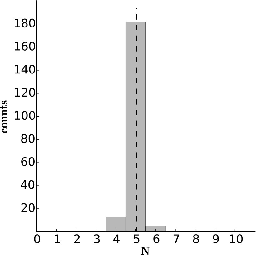
The bootstrap results show that the parameters were determined precisely, except for a small underestimate of N throughout and a small bias toward slower in set 2 (Fig. 3). This set has a faster blinking rate than the other two sets. When we had simulated the synthetic data, we imposed a 50-ms time bin on our simulated data (to mimic the time resolution, i.e., camera rate, of PALM experiments). In Fig. 4 we show that this bias toward smaller N is due to missed transitions in the presence of fast blinking and low temporal resolution. In other words, as we increase the resolution to 5 ms, the bias in the estimate of N indeed vanishes.
Fig. 4.
Histogram of bootstrapping results from simulated data set 2 with 5-ms time bins. We followed the same procedure as in Fig. 3 except we now used 5-ms—as opposed to 50-ms—time bins.
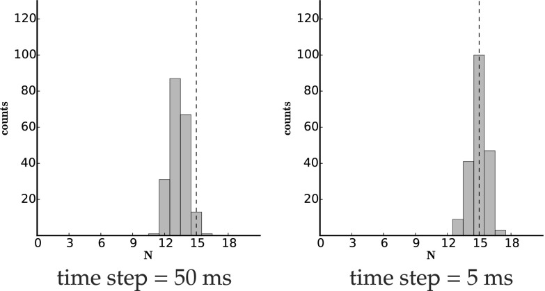
Finally, Fig. 5 shows that if the values for the rates are known, we can use the PALM trajectory data to find the only unknown—namely, N. We show this to be the case in Fig. 5 for the challenging parameter set 1 both with 5-ms and 50-ms temporal resolution where the theoretical N value is set to 15. Again, the simulation with a resolution to 5 ms is sharply peaked at the correct answer.
Fig. 5.
Histogram of N obtained by assuming rates. We demonstrate that we can accurately determine N if the rates are known. We use parameters from set 1 from Table 1 and use the simulated data to determine N (and not the rates). (Left) Shown with 50-ms time resolution (and therefore underestimated N). (Right) Improvement afforded by smaller time resolution (5 ms).
Analysis of in Vitro Data.
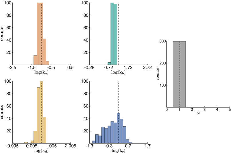
In addition to the simulated data presented above, we analyzed the in vitro data of Lee et al. (40). In this data set (which includes 1,000 traces), biotinylated Dendra2 molecules were immobilized on a streptavidin-coated glass coverslip, in a manner such that oligomerization was negligible and molecules were spatially well separated enough to be detected individually . The sample was simultaneously illuminated with 405-nm and 561-nm lasers to activate (from a precursor state to I) and then excite (from I to A) the Dendra2 molecules, respectively, until all of the molecules were photobleached (see Lee et al. (40) for further details). Individual emission bursts from the EMCCD output were processed into single-molecule time traces for analysis as described in ref. 40.
We simultaneously extracted the four kinetic rates (, , , ) and found that Dendra2 blinking probability is low ; its behavior most closely resembles that of set 3 of our simulated data. Dendra2 molecules are more likely to photobleach upon activation than blink. Our N distribution is sharply peaked at 1 (Fig. 6), as expected for this data set, because the experiments were designed to separate and isolate Dendra2 molecules on the coverslip. Our rate estimates (drawn from 300 bootstrap iterations) compare well with those of Lee et al. (40), who found a similar blinking rate (Table 2). Our results differ from their results most significantly for , the rate of recovery from D to A. Lee et al. (40) fit the distribution of fluorescence-off times to determine and found that the distribution fit poorly to a single exponential, but that it was well fit by a double exponential . The poor fit to a single exponential agrees with the fact that our histogram of is heavy tailed toward slower rates (Fig. 6). Their findings and ours suggest that the kinetic model of Dendra2 (Fig. 1) should be amended to two dark states rather than one. We will explore the possibility of including more dark states, and the implication of uniquely identifying a model when using more dark states, in future work.
Fig. 6.
Histogram of bootstrapping results from in vitro data. Histogram of bootstrapping results from in vitro data with 1,000 time traces (300 bootstrap iterations). The dashed lines show the parameter values from Lee et al. (40).
Table 2.
In vitro Dendra2 kinetic rates
| Rate constant | Our analysis | Lee et al. (40) |
| 0.009 | 0.01 | |
| 2.8 | 3.2 | |
| 0.87 | 1.6 | |
| n/a | 18, | |
| 9.2 | 16.6 | |
| 0.3 | 0.2 |
In vitro Dendra2 kinetic rates from the current AMM analysis and from Lee et al. (40). Rates in units of Hz.
Missed Transitions May Be Necessary in Tackling Larger Data Sets.
To tackle more challenging data sets, we need to correct for missed transitions when PA-FP residence times in the dark or active state are on the order of the temporal resolution or data acquisition time (the dead time, ). The mathematical details are relegated to Materials and Methods. Typically, the lower bound for this time resolution is limited by the camera’s acquisition rate, i.e., the frame integration time.
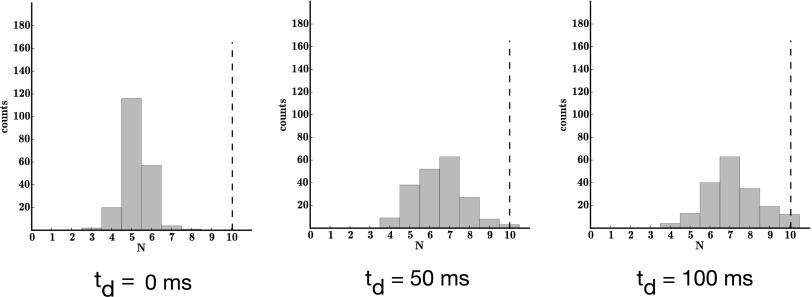
In Fig. 7, Left, we show a distribution over N obtained by combining 10 traces of the from the in vitro data to generate more challenging yet controlled data sets. We generated 1,000 of such traces. When , we underestimate N by a factor of ∼2 (even after 200 bootstrap iterations). This underestimation is most likely due to the missed transitions of the active state rather than of the dark state. Because the mean dwell time in the active state (83 ms ) from Table 2 is about as long as the data integration time (50 ms), we expect to miss about half the transitions to the active state, which agrees well with our result ( using instead of the expected ; Fig. 7). By contrast, the dwell in the dark (1,100 ms) is much larger (∼20 times) than this integration time.
Fig. 7.
Increasing the dead time, , helps approximately correct for missed transitions. We combine 10 in vitro traces and use the combined traces to determine rates and N (whose theoretical value should be ). We generated 1,000 of such traces (with 200 bootstrap iterations). The distribution over N is shown for increasing values of . Dendra2 has a dwell time in the bright state, which is on average approximately as long as the time resolution of experiment (50 ms). Thus, when is zero, approximately half the transitions to the bright state are missed. As increases, our estimate for N improves. Fig. 4 shows that PA-FPs with kinetics slower than the integration time should improve the estimate for N.
We did not undercount when we considered the (Fig. 6) case because the probability of observing exactly is zero because the first fluorescent peak is automatically counted as one emission burst, which obviously corresponds to the activation of a new molecule. We did not overcount because our theory correctly differentiates between blinks and new photoactivations (as benchmarked for our simulated data sets).
To approximately correct for the undercounting when N is larger than 1, we increased to 50 ms, which considerably improves our N estimate (Fig. 7).
Next, if we set the dead time closer to the active-state dwell time, the distribution shifts still further toward the correct value (Fig. 7).
To avoid using this approximate treatment, a goal should be to develop PA-FPs that blink with kinetics slower than the data’s acquisition rate.
Making Use of Intensity Measurements.
Previously, we showed how to correct for missed transitions in dealing with real data sets. Here we describe how to use fluorescence intensity data by separating bright states into several distinct aggregates also relevant to analyzing real data sets (Fig. 8).
Fig. 8.
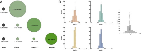
Using intensity measurements can improve the estimate for N. (A) When we can observe, in principle, a fluorescence intensity ranging from one to five bright (if all PA-FPs are on simultaneously). Here we show how many states coincide with the different fluorescence intensities up to three simultaneously bright. (B) We show that we can take advantage of the intensity measurements to compute a correctly centered distribution for N (using 200 synthetic traces with 200 bootstrap iterations).
Fig. 8A shows the number of states in each aggregated class for fluorophores. The top row groups all bright macrostates into one class. The second row splits the bright macrostates into two bright classes, and the bottom row further splits them into a third bright class. The class sizes have a practical consequences: they determine the sizes of the transition matrix submatrices (discussed in Materials and Methods), which determine the computational cost of computing the matrix exponentials and, ultimately, the computational cost of parameter extraction.
The method recovers correctly (after 200 bootstrap iterations) when there are two bright aggregates, corresponding to one fluorophore active and more than one fluorophore active, respectively (Fig. 8B). A mathematical formalism is detailed in Materials and Methods.
Using the same number of synthetic traces and bootstrap iterations, we then extracted rates and N for a larger simulated data set with two observable bright aggregates. With a 50-ms time resolution, the rates were correctly extracted but N was underestimated because some transitions are missed. By regenerating simulated data with 5-ms time resolution, the rates are also correctly extracted and the estimate of N improves, but the distribution remains relatively broad because the data are probed to extract all rates as well as N (Fig. 9). The estimate for N sharpens dramatically, even when trying to estimate larger N, when information on the rates is provided and the data are instead entirely focused on estimating N more precisely (Fig. 5). All code used to generate the results can be obtained by emailing the corresponding author.
Fig. 9.
Intensity measurements become particularly useful when estimating rates and N for larger N. Here we used simulated set 1 with (200 synthetic traces with 200 bootstrap iterations). If the data are instead focused on determining only N, rather than N and the rates, the distribution over N becomes dramatically sharper even for larger N (Fig. 5).
Discussion
Common biochemical/biophysical methods used to establish the stoichiometry of protein complexes often lack single molecule resolution. For example, in the ion-channel literature the following methods are common: densitometry of silver-stained and Western-blotted protein complexes (in quantifying atrial inward rectifying potassium channel complex stoichiometry) (50); voltage-clamp electrical recordings [combined with channel inhibitors release to count potassium voltage gated channel (KCNE) subunits] (7); LC-MS (in counting subunit e used in bovine heart mitochondria ATP synthase self-association) (51); coimmunoprecipitation/immunocytochemistry (to assess colocalization of potassium voltage-gated channels such as KCNE2 to KCNQ1 and KCNE1 in cardiomyocytes) (17).
Fluorescence-based methods are also common in enumerating proteins but have severe limitations. For instance, flow cytometry (52, 53) yields estimates for intracellular protein number, but provides no spatial resolution and is less accurate for proteins numbering less than a few hundred (53). By contrast, quantitative fluorescence microscopy (54–56), which is diffraction limited, provides a maximum spatial resolution of a few hundred nanomoles and is commonly used in protein counting, but still provides an order of magnitude less resolution than PALM or STORM (stochastic optical reconstruction microscopy), another SR technique. Using quantitative fluorescence, Joglekar et al. (54) counted proteins in the kinetochore of budding yeast using the fluorescence intensity from tagged Cse4p (57–59) as a fluorescence intensity standard. This indirect method can lead to counting errors because standards themselves can be poorly characterized (18, 19).
Stepwise photobleaching methods, in turn, count proteins by monitoring discrete fluorescence intensity drops as individual proteins photobleach over one ROI. This method was used to count KCNE1s in the cardiac channel (5). Photobleaching does not require fluorescence standards but is still diffraction limited (20–23). Furthermore, the noise inherent to photobleaching data limits the method to complexes with less than 5–6 proteins (21).
By comparison, the method presented here provides a principled recipe for enumerating PA-FPs while gathering critical photophysical properties of the PA-FPs directly and self-consistently from the same SR data set used to determine N.
A qualitative reason explaining why likelihood functions peak at the correct value of N (Fig. S3) is illustrated with the following example. Suppose we start by guessing that all fluorescence spikes in a time trace are due to one PA-FP (i.e., ). Thus, all events, except the first photoactivation, are blinks. Assuming we only have a single D state, all waiting times between successive fluorescence spikes should therefore be sampled from this distribution: . However, if we have many PA-FPs, not all waiting times will be sampled from , and the likelihood of will be small. We can repeat a similar reasoning for any N value.
Another decisive advantage of our method is its ability to generate entire distributions of N for a given complex; this is particularly relevant given that protein complex stoichiometry may vary from complex to complex based on the dissociation constant of the various subunits in those complexes (5, 60), tissue development, and even its disease state (8, 61, 62). Developing therapeutic agents against some heart diseases, for instance, may require a quantitative assessment of protein complex composition in living tissues (7, 62–64) and finding drugs to restore native complex stoichiometries is one such strategy (8, 62).
Our method is a first step in the quantitative determination of N from SR data, it includes the treatment of the “missed event problem” and shows how one can take advantage of intensity measurements.
Materials and Methods
States of the Model.
We assume that each fluorophore is independent of the others: the state of one fluorophore does not affect the state of any other fluorophore. We describe the state of a system of N fluorophores as a vector of the populations of the inactive, active, dark, and photobleached states: . To avoid confusion, we will use the term “microstate” to refer to the state of a single fluorophore (i.e., I, A, D, or B), and “macrostate” to refer to a population vector that describes the collection of fluorophores. For example, macrostate i for a collection of two PA-FPs in which both PA-FPs are inactive would be . The set of all macrostates is , where each in S is a population vector and M is the total number of macrostates.
Computing M is a common combinatorial problem: the number of unique ways to partition N indistinguishable objects into x bins. In this case, the objects are PA-FPs and the bins are the microstates. There are four microstates, so .
| [1] |
For example, if the collection contains two fluorophores, the following 10 macrostates (obtained from ) are available.
We model the collection of PA-FPs as an AMM. As shown in Table S1, each macrostate belongs to an aggregated class, either dark or bright. Macrostates with at least one active PA-FP are assigned to the bright class. Macrostates with zero active PA-FPs are assigned to the dark class.
Here, the bright class corresponds to the detection of fluorescence and the dark class corresponds to the absence of fluorescence. The aggregated classes are necessary because PALM experiments cannot distinguish between the various dark states. The dark and bright classes here are analogous to the closed and open classes in the ion channel AMMs.
There can be multiple bright classes as there can be multiple levels of fluorescence that are observable: bright, bright2, bright3, …, brightN, as shown in Fig. 8.
The number of macrostates grows exponentially (Fig. S4) with N, which is a concern for the numerical calculations discussed in the results section; the computational time of the likelihood depends on the number of macrostates. As such, we define a quantity , which represents the maximum number of PA-FPs we allow to be simultaneously photoactive. We use this quantity as a way to tune the size of the state space to save on computational time in situations where we expect photoactivation events to be well separated in time.
Model Kinetics.
The transition rate from macrostate to macrostate is simply the transition rate for one PA-FP multiplied by a combinatoric factor for the population of the appropriate microstate. The macrostate transition rates are summarized in Table S2.
The dynamics of the PA-FP AMM are governed by a rate matrix, . Each off-diagonal matrix element equals the transition rate of . The diagonal elements are set so that each row sums to zero: . The macrostate transition probabilities at any time t are given by the Kolmogorov equation (34):
| [2] |
whose solution is given by
| [3] |
In the case of dark and bright observation classes, we can partition the rate matrix Q into four submatrices, based on the dark (subscript d) and bright (subscript b) aggregated classes:
| [4] |
The submatrix contains the rates for transitions from states in class d to other states in class d; contains the rates for transitions from the states in class d to the states in class b. The other two submatrices are similarly defined.
Another possibility would be that multiple levels of fluorescence are observable: bright1, bright2, bright3, etc. For example, in the case of two bright aggregated classes, macrostates with would be grouped into the bright1 class, which we denote . Macrostates with would be grouped into the bright2 class, which we denote . By extension, if three intensity levels were resolvable, would contain macrostates with and class would contain macrostates with . In the case of one dark class and two bright observation classes, our rate matrix would be partitioned into nine submatrices:
Having multiple bright aggregates is advantageous because it shrinks the size of the largest submatrix in the likelihood calculation. Furthermore, if the time traces infrequently visit the higher brightness classes, then fewer exponentiations of the largest submatrix will be necessary.
Likelihood Function.
The likelihood function that we describe in this section provides an answer to the following question: Given a kinetic model and a set of kinetic rates, what’s the likelihood of observing the data? Our goal is to determine the kinetic rates and N that maximize the likelihood function, i.e., maximize the likelihood of observing the data that was collected by PALM.
Suppose we have a trajectory of L dwells representing the dynamics of a collection of N PA-FPs. Associated with each dwell is an observed aggregated class and a dwell time. The set of observation classes is . The set of dwell times is . So, during dwell i we observe class for duration . See Fig. 10 for an illustration. The probability densities for dwelling in the dark class for time t and then transitioning to the bright class are given by the elements of the following matrix:
| [5] |
Fig. 10.
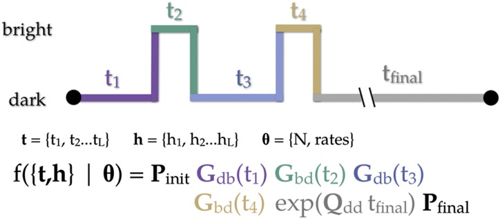
Likelihood function. An idealized time trace. Each dwell is color-coded with its corresponding term in the likelihood function.
The element of is the probability density of entering class d from its state, dwelling in class d for time t, and then transitioning to the state of class b.
When we have missed transitions, we implement renormalized transition matrices—instead of transition matrices like those given by Eq. 5 —that account for missed transitions to the bright state, say, by resuming over all possible missed events (37, 65)
Next, we wish to calculate the likelihood of the dwell trajectory h, given the model parameters θ, where θ is the set of parameters (N and the transition rates) that go into the rate matrix Q. The likelihood function then reads as follows:
| [6] |
where is a probability vector with all probability density in the fully inactive macrostate. The parameters, θ, determine the elements of the rate matrix Q. The final factor of comes from the fact that all of the PA-FPs irreversibly photobleach by the end of the trajectory. After all photobleaching events occur, the system will dwell in the dark class indefinitely; we represent this with a long final dwell in the dark class for time s. is a probability vector with all probability density in the fully photobleached macrostate.
Numerical Evaluation of the Likelihood Function.
Our goal is to find the set of parameters that maximize the likelihood function given the data (a dwell trajectory represented by t and h; in practice, this is accomplished by minimizing with respect to the rates for a fixed value of N, and then repeating this process for other values of N). The optimization is performed in Python using the limited-memory Broyden-Fletcher-Goldfarb-Shanno (BFGS) minimizer, implemented in Scipy (66). BFGS is a quasi-Newton method that performs well on nonsmooth optimization problems. The computational time is plotted in Fig. S5. The scaling depends on , and it is advantageous to set to a small value when possible (when activation events are well separated).
As an aside, we point out that is still distinct from thresholding methods. Consider the following scenario: a PA-FP activates, and then blinks. Whereas the first PA-FP is in the dark state, a second PA-FP activates and photobleaches before the first molecule recovers from blinking. This scenario would still obey , but it would be forbidden in thresholding.
To determine whether likelihood maximization runs converge to the correct parameter values, as a preliminary test we computed 1D slices in parameter space around the true value of each parameter. Each panel of Fig. S3 was obtained by holding four of the five parameters (, , , , and N) constant at their true values and then varying the remaining parameter over a range encompassing its true value. We see that the four kinetic rates are peaked in the correct location at their true values. In the 1D slice for N, we see a maximum (as determined by the value of the likelihood function) that spans and .
Next, we assessed the ability of the numerical maximization procedure to converge to the correct parameter values. The 1D slices discussed above suggest that the likelihood function maximum is in the correct region of parameter space, but a separate question is, Can we simultaneously determine all five parameters? We found that the likelihood-maximization procedure converges to the correct kinetic rates within 100 cycles. Fig. S6 shows the convergence of the rate estimates from one of the maximization runs. For simulated fast (set 2) and slow blinking (set 3), we found that convergence of the likelihood maximization also occurred within ∼100 cycles.
Supplementary Material
Acknowledgments
We thank S. H. Lee and A. Lee for providing the Dendra2 in vitro data and for numerous helpful discussions about PALM and the blinking problem. Support for this work was provided by a National Science Foundation (NSF) Graduate Research Fellowship (to G.C.R.); the Burroughs Wellcome Fund and NSF Grant MCB-1412259 (to S.P.); and the Howard Hughes Medical Institute and NIH Grant R01-GM032543 (to C.B.).
Footnotes
The authors declare no conflict of interest.
This article is a PNAS Direct Submission.
See Commentary on page 304.
This article contains supporting information online at www.pnas.org/lookup/suppl/doi:10.1073/pnas.1408071112/-/DCSupplemental.
References
- 1.Zamft B, Bintu L, Ishibashi T, Bustamante C. Nascent RNA structure modules the transcription dynamics of RNA polymerases. Proc Natl Acad Sci USA. 2012;109(23):8948–8953. doi: 10.1073/pnas.1205063109. [DOI] [PMC free article] [PubMed] [Google Scholar]
- 2.Boyer PD. The ATP synthase—a splendid molecular machine. Annu Rev Biochem. 1997;66:717–749. doi: 10.1146/annurev.biochem.66.1.717. [DOI] [PubMed] [Google Scholar]
- 3.Cimini D. Merotelic kinetochore orientation, aneuploidy, and cancer. Biochimica et Biophysica Acta Rev Cancer. 2008;1786(1):32–40. doi: 10.1016/j.bbcan.2008.05.003. [DOI] [PubMed] [Google Scholar]
- 4.Cai S, O’Connell CB, Khodjakov A, Walczak CE. Chromosome congression in the absence of kinetochore fibres. Nat Cell Biol. 2009;11(7):832–838. doi: 10.1038/ncb1890. [DOI] [PMC free article] [PubMed] [Google Scholar]
- 5.Nakajo K, Ulbrich MH, Kubo Y, Isacoff EY. Stoichiometry of the KCNQ1– KCNE1 ion channel complex. Proc Natl Acad Sci USA. 2010;107(44):18862–18867. doi: 10.1073/pnas.1010354107. [DOI] [PMC free article] [PubMed] [Google Scholar]
- 6.Osteen JD, Sampson KJ, Kass RS. The cardiac IKs channel, complex indeed. Proc Natl Acad Sci USA. 2010;107(44):18751–18752. doi: 10.1073/pnas.1014150107. [DOI] [PMC free article] [PubMed] [Google Scholar]
- 7.Morin TJ, Kobertz WR. Counting membrane-embedded KCNE beta-subunits in functioning K+ channel complexes. Proc Natl Acad Sci USA. 2008;105(5):1478–1482. doi: 10.1073/pnas.0710366105. [DOI] [PMC free article] [PubMed] [Google Scholar]
- 8.Yano M, et al. Altered stoichiometry of FKBP12.6 versus ryanodine receptor as a cause of abnormal Ca(2+) leak through ryanodine receptor in heart failure. Circulation. 2000;102(17):2131–2136. doi: 10.1161/01.cir.102.17.2131. [DOI] [PubMed] [Google Scholar]
- 9.Lacoste TD, et al. Ultrahigh-resolution multicolor colocalization of single fluorescent probes. Proc Natl Acad Sci USA. 2000;97(17):9461–9466. doi: 10.1073/pnas.170286097. [DOI] [PMC free article] [PubMed] [Google Scholar]
- 10.Gordon MP, Ha T, Selvin PR. Single-molecule high-resolution imaging with photobleaching. Proc Natl Acad Sci USA. 2004;101(17):6462–6465. doi: 10.1073/pnas.0401638101. [DOI] [PMC free article] [PubMed] [Google Scholar]
- 11.Huang B, Bates M, Zhuang X. Super-resolution fluorescence microscopy. Annu Rev Biochem. 2009;78:993–1016. doi: 10.1146/annurev.biochem.77.061906.092014. [DOI] [PMC free article] [PubMed] [Google Scholar]
- 12.Qu X, Wu D, Mets L, Scherer NF. Nanometer-localized multiple single-molecule fluorescence microscopy. Proc Natl Acad Sci USA. 2004;101(31):11298–11303. doi: 10.1073/pnas.0402155101. [DOI] [PMC free article] [PubMed] [Google Scholar]
- 13.Dedecker P, De Schryver FC, Hofkens J. Fluorescent proteins: Shine on, you crazy diamond. J Am Chem Soc. 2013;135(7):2387–2402. doi: 10.1021/ja309768d. [DOI] [PubMed] [Google Scholar]
- 14.Wiedenmann J, et al. EosFP, a fluorescent marker protein with UV-inducible green-to-red fluorescence conversion. Proc Natl Acad Sci USA. 2004;101(45):15905–15910. doi: 10.1073/pnas.0403668101. [DOI] [PMC free article] [PubMed] [Google Scholar]
- 15.Gurskaya NG, et al. Engineering of a monomeric green-to-red photoactivatable fluorescent protein induced by blue light. Nat Biotechnol. 2006;24(4):461–465. doi: 10.1038/nbt1191. [DOI] [PubMed] [Google Scholar]
- 16.Fron E, et al. Revealing the excited-state dynamics of the fluorescent protein Dendra2. J Phys Chem B. 2013;117(8):2300–2313. doi: 10.1021/jp309219m. [DOI] [PubMed] [Google Scholar]
- 17.Wu DM, et al. KCNE2 is colocalized with KCNQ1 and KCNE1 in cardiac myocytes and may function as a negative modulator of I(Ks) current amplitude in the heart. Heart Rhythm. 2006;3(12):1469–1480. doi: 10.1016/j.hrthm.2006.08.019. [DOI] [PubMed] [Google Scholar]
- 18.Coffman VC, Wu P, Parthun MR, Wu JQ. CENP-A exceeds microtubule attachment sites in centromere clusters of both budding and fission yeast. J Cell Biol. 2011;195(4):563–572. doi: 10.1083/jcb.201106078. [DOI] [PMC free article] [PubMed] [Google Scholar]
- 19.Lawrimore J, Bloom KS, Salmon ED. Point centromeres contain more than a single centromere-specific Cse4 (CENP-A) nucleosome. J Cell Biol. 2011;195(4):573–582. doi: 10.1083/jcb.201106036. [DOI] [PMC free article] [PubMed] [Google Scholar]
- 20.Leake MC, et al. Stoichiometry and turnover in single, functioning membrane protein complexes. Nature. 2006;443(7109):355–358. doi: 10.1038/nature05135. [DOI] [PubMed] [Google Scholar]
- 21.Ulbrich MH, Isacoff EY. Subunit counting in membrane-bound proteins. Nat Methods. 2007;4(4):319–321. doi: 10.1038/NMETH1024. [DOI] [PMC free article] [PubMed] [Google Scholar]
- 22.Hastie P, et al. AMPA receptor/TARP stoichiometry visualized by single-molecule subunit counting. Proc Natl Acad Sci USA. 2013;110(13):5163–5168. doi: 10.1073/pnas.1218765110. [DOI] [PMC free article] [PubMed] [Google Scholar]
- 23.Delalez NJ, et al. Signal-dependent turnover of the bacterial flagellar switch protein FliM. Proc Natl Acad Sci USA. 2010;107(25):11347–11351. doi: 10.1073/pnas.1000284107. [DOI] [PMC free article] [PubMed] [Google Scholar]
- 24.Heilemann M, Dedecker P, Hofkens J, Sauer M. Photoswitches: Key molecules for subdiffraction-resolution fluorescence imaging and molecular quantification. Laser Photon Rev. 2009;3(1-2):180–202. [Google Scholar]
- 25.Roy A, Field MJ, Adam V, Bourgeois D. The nature of transient dark states in a photoactivatable fluorescent protein. J Am Chem Soc. 2011;133(46):18586–18589. doi: 10.1021/ja2085355. [DOI] [PubMed] [Google Scholar]
- 26.Schäfer LV, Groenhof G, Boggio-Pasqua M, Robb MA, Grubmüller H. Chromophore protonation state controls photoswitching of the fluoroprotein asFP595. PLOS Comput Biol. 2008;4(3):e1000034. doi: 10.1371/journal.pcbi.1000034. [DOI] [PMC free article] [PubMed] [Google Scholar]
- 27.Griesbeck O, Baird GS, Campbell RE, Zacharias DA, Tsien RY. Reducing the environmental sensitivity of yellow fluorescent protein. Mechanism and applications. J Biol Chem. 2001;276(31):29188–29194. doi: 10.1074/jbc.M102815200. [DOI] [PubMed] [Google Scholar]
- 28.McKinney SA, Murphy CS, Hazelwood KL, Davidson MW, Looger LL. A bright and photostable photoconvertible fluorescent protein. Nat Methods. 2009;6(2):131–133. doi: 10.1038/nmeth.1296. [DOI] [PMC free article] [PubMed] [Google Scholar]
- 29.Lukyanov KA, Chudakov DM, Lukyanov S, Verkhusha VV. Innovation: Photoactivatable fluorescent proteins. Nat Rev Mol Cell Biol. 2005;6(11):885–891. doi: 10.1038/nrm1741. [DOI] [PubMed] [Google Scholar]
- 30.Lippincott-Schwartz J, Patterson GH. Development and use of fluorescent protein markers in living cells. Science. 2003;300(5616):87–91. doi: 10.1126/science.1082520. [DOI] [PubMed] [Google Scholar]
- 31.Dickson RM, Cubitt AB, Tsien RY, Moerner WE. On/off blinking and switching behaviour of single molecules of green fluorescent protein. Nature. 1997;388(6640):355–358. doi: 10.1038/41048. [DOI] [PubMed] [Google Scholar]
- 32.Remington SJ. Fluorescent proteins: Maturation, photochemistry and photophysics. Curr Opin Struct Biol. 2006;16(6):714–721. doi: 10.1016/j.sbi.2006.10.001. [DOI] [PubMed] [Google Scholar]
- 33.Chudakov DM, Feofanov AV, Mudrik NN, Lukyanov S, Lukyanov KA. Chromophore environment provides clue to “kindling fluorescent protein” riddle. J Biol Chem. 2003;278(9):7215–7219. doi: 10.1074/jbc.M211988200. [DOI] [PubMed] [Google Scholar]
- 34.Colquhoun D, Hawkes AG. On the stochastic properties of single ion channels. Proc R Soc Lond B Biol Sci. 1981;211(1183):205–235. doi: 10.1098/rspb.1981.0003. [DOI] [PubMed] [Google Scholar]
- 35.Kienker P. Equivalence of aggregated Markov models of ion-channel gating. Proc R Soc Lond B Biol Sci. 1989;236(1284):269–309. doi: 10.1098/rspb.1989.0024. [DOI] [PubMed] [Google Scholar]
- 36.Colquhoun D, Hawkes AG, Srodzinski K. Joint distributions of apparent open and shut times of single-ion channels and maximum likelihood fitting of mechanisms. Philos Trans R Soc A-Math Phys Eng Sci. 1996;354:2555–2590. [Google Scholar]
- 37.Qin F, Auerbach A, Sachs F. Estimating single-channel kinetic parameters from idealized patch-clamp data containing missed events. Biophys J. 1996;70(1):264–280. doi: 10.1016/S0006-3495(96)79568-1. [DOI] [PMC free article] [PubMed] [Google Scholar]
- 38.Qin F, Auerbach A, Sachs F. Maximum likelihood estimation of aggregated Markov processes. Proc Biol Sci. 1997;264(1380):375–383. doi: 10.1098/rspb.1997.0054. [DOI] [PMC free article] [PubMed] [Google Scholar]
- 39.Coltharp C, Kessler RP, Xiao J. Accurate construction of photoactivated localization microscopy (PALM) images for quantitative measurements. PLoS ONE. 2012;7(12):e51725. doi: 10.1371/journal.pone.0051725. [DOI] [PMC free article] [PubMed] [Google Scholar]
- 40.Lee SH, Shin JY, Lee A, Bustamante C. Counting single photoactivatable fluorescent molecules by photoactivated localization microscopy (PALM) Proc Natl Acad Sci USA. 2012;109(43):17436–17441. doi: 10.1073/pnas.1215175109. [DOI] [PMC free article] [PubMed] [Google Scholar]
- 41.Annibale P, Vanni S, Scarselli M, Rothlisberger U, Radenovic A. Identification of clustering artifacts in photoactivated localization microscopy. Nat Methods. 2011;8(7):527–528. doi: 10.1038/nmeth.1627. [DOI] [PubMed] [Google Scholar]
- 42.Annibale P, Vanni S, Scarselli M, Rothlisberger U, Radenovic A. Quantitative photo activated localization microscopy: Unraveling the effects of photoblinking. PLoS ONE. 2011;6(7):e22678. doi: 10.1371/journal.pone.0022678. [DOI] [PMC free article] [PubMed] [Google Scholar]
- 43.Gillespie DT. Exact stochastic simulation of coupled chemical reactions. J Phys Chem. 1977;81(25):2340–2361. [Google Scholar]
- 44.Durisic N, Laparra-Cuervo L, Sandoval-Álvarez A, Borbely JS, Lakadamyali M. Single-molecule evaluation of fluorescent protein photoactivation efficiency using an in vivo nanotemplate. Nat Methods. 2014;11(2):156–162. doi: 10.1038/nmeth.2784. [DOI] [PubMed] [Google Scholar]
- 45.Zhang L, et al. Method for real-time monitoring of protein degradation at the single cell level. Biotechniques. 2007;42(4):446–450, 448, 450. doi: 10.2144/000112453. [DOI] [PubMed] [Google Scholar]
- 46.McKinney SA, Murphy CS, Hazelwood KL, Davidson MW, Looger LL. A bright and photostable photoconvertible fluorescent protein. Nat Methods. 2009;6(2):131–133. doi: 10.1038/nmeth.1296. [DOI] [PMC free article] [PubMed] [Google Scholar]
- 47.Johnston K, et al. Vertebrate kinetochore protein architecture: Protein copy number. J Cell Biol. 2010;189(6):937–943. doi: 10.1083/jcb.200912022. [DOI] [PMC free article] [PubMed] [Google Scholar]
- 48.Efron B. Bootstrap methods: Another look at the jackknife. Ann Stat. 1979;7(1):1–26. [Google Scholar]
- 49.Efron B, Tibshirani R. Statistical data analysis in the computer age. Science. 1991;253(5018):390–395. doi: 10.1126/science.253.5018.390. [DOI] [PubMed] [Google Scholar]
- 50.Corey S, Krapivinsky G, Krapivinsky L, Clapham DE. Number and stoichiometry of subunits in the native atrial G-protein-gated K+ channel, IKACh. J Biol Chem. 1998;273(9):5271–5278. doi: 10.1074/jbc.273.9.5271. [DOI] [PubMed] [Google Scholar]
- 51.Bisetto E, et al. Functional and stoichiometric analysis of subunit e in bovine heart mitochondrial F(0)F(1)ATP synthase. J Bioenerg Biomembr. 2008;40(4):257–267. doi: 10.1007/s10863-008-9183-5. [DOI] [PubMed] [Google Scholar]
- 52.Huh WK, et al. Global analysis of protein localization in budding yeast. Nature. 2003;425(6959):686–691. doi: 10.1038/nature02026. [DOI] [PubMed] [Google Scholar]
- 53.Newman JR, et al. Single-cell proteomic analysis of S. cerevisiae reveals the architecture of biological noise. Nature. 2006;441(7095):840–846. doi: 10.1038/nature04785. [DOI] [PubMed] [Google Scholar]
- 54.Joglekar AP, Salmon ED, Bloom KS. Counting kinetochore protein numbers in budding yeast using genetically encoded fluorescent proteins. Methods Cell Biol. 2008;85:127–151. doi: 10.1016/S0091-679X(08)85007-8. [DOI] [PMC free article] [PubMed] [Google Scholar]
- 55.Wu JQ, McCormick CD, Pollard TD. Chapter 9: Counting proteins in living cells by quantitative fluorescence microscopy with internal standards. Methods Cell Biol. 2008;89:253–273. doi: 10.1016/S0091-679X(08)00609-2. [DOI] [PubMed] [Google Scholar]
- 56.Coffman VC, Wu JQ. Counting protein molecules using quantitative fluorescence microscopy. Trends Biochem Sci. 2012;37(11):499–506. doi: 10.1016/j.tibs.2012.08.002. [DOI] [PMC free article] [PubMed] [Google Scholar]
- 57.Collins KA, Furuyama S, Biggins S. Proteolysis contributes to the exclusive centromere localization of the yeast Cse4/CENP-A histone H3 variant. Curr Biol. 2004;14(21):1968–1972. doi: 10.1016/j.cub.2004.10.024. [DOI] [PubMed] [Google Scholar]
- 58.Meluh PB, Yang P, Glowczewski L, Koshland D, Smith MM. Cse4p is a component of the core centromere of Saccharomyces cerevisiae. Cell. 1998;94(5):607–613. doi: 10.1016/s0092-8674(00)81602-5. [DOI] [PubMed] [Google Scholar]
- 59.Joglekar AP, Bouck DC, Molk JN, Bloom KS, Salmon ED. Molecular architecture of a kinetochore-microtubule attachment site. Nat Cell Biol. 2006;8(6):581–585. doi: 10.1038/ncb1414. [DOI] [PMC free article] [PubMed] [Google Scholar]
- 60.Jiang M, et al. Dynamic partnership between KCNQ1 and KCNE1 and influence on cardiac IKs current amplitude by KCNE2. J Biol Chem. 2009;284(24):16452–16462. doi: 10.1074/jbc.M808262200. [DOI] [PMC free article] [PubMed] [Google Scholar]
- 61.Bendahhou S, et al. In vitro molecular interactions and distribution of KCNE family with KCNQ1 in the human heart. Cardiovasc Res. 2005;67(3):529–538. doi: 10.1016/j.cardiores.2005.02.014. [DOI] [PubMed] [Google Scholar]
- 62.Yano M, et al. FKBP12.6-mediated stabilization of calcium-release channel (ryanodine receptor) as a novel therapeutic strategy against heart failure. Circulation. 2003;107(3):477–484. doi: 10.1161/01.cir.0000044917.74408.be. [DOI] [PubMed] [Google Scholar]
- 63.Cingolani E, et al. Gene therapy to inhibit the calcium channel beta subunit: Physiological consequences and pathophysiological effects in models of cardiac hypertrophy. Circ Res. 2007;101(2):166–175. doi: 10.1161/CIRCRESAHA.107.155721. [DOI] [PubMed] [Google Scholar]
- 64.Yu H, et al. Dynamic subunit stoichiometry confers a progressive continuum of pharmacological sensitivity by KCNQ potassium channels. Proc Natl Acad Sci USA. 2013;110(21):8732–8737. doi: 10.1073/pnas.1300684110. [DOI] [PMC free article] [PubMed] [Google Scholar]
- 65.Roux B, Sauvé R. A general solution to the time interval omission problem applied to single channel analysis. Biophys J. 1985;48(1):149–158. doi: 10.1016/S0006-3495(85)83768-1. [DOI] [PMC free article] [PubMed] [Google Scholar]
- 66.Zhu CY, Byrd RH, Lu PH, Nocedal J. Algorithm 778: L-BFGS-B: Fortran subroutines for large-scale bound-constrained optimization. ACM Trans Math Softw. 1997;23(4):550–560. [Google Scholar]
Associated Data
This section collects any data citations, data availability statements, or supplementary materials included in this article.


